
 Submit a Paper
 Propose a Special lssue
 Open Access
ARTICLE

A Unified Model Fusing Region of Interest Detection and Super Resolution for Video Compression
1 School of Computer and Cyber Sciences, Communication University of China, Beijing, 100024, China
2 Cable Television Technology Research Institute, Academy of Broadcasting Science, Beijing, 100866, China
* Corresponding Author: Ying Xu. Email:
(This article belongs to the Special Issue: Edge Computing in Advancing the Capabilities of Smart Cities)
Computers, Materials & Continua 2024, 79(3), 3955-3975. https://doi.org/10.32604/cmc.2024.049057
Received 26 December 2023; Accepted 12 March 2024; Issue published 20 June 2024
 View Full Text
 Download PDF
Abstract
High-resolution video transmission requires a substantial amount of bandwidth. In this paper, we present a novel video processing methodology that innovatively integrates region of interest (ROI) identification and super-resolution enhancement. Our method commences with the accurate detection of ROIs within video sequences, followed by the application of advanced super-resolution techniques to these areas, thereby preserving visual quality while economizing on data transmission. To validate and benchmark our approach, we have curated a new gaming dataset tailored to evaluate the effectiveness of ROI-based super-resolution in practical applications. The proposed model architecture leverages the transformer network framework, guided by a carefully designed multi-task loss function, which facilitates concurrent learning and execution of both ROI identification and resolution enhancement tasks. This unified deep learning model exhibits remarkable performance in achieving super-resolution on our custom dataset. The implications of this research extend to optimizing low-bitrate video streaming scenarios. By selectively enhancing the resolution of critical regions in videos, our solution enables high-quality video delivery under constrained bandwidth conditions. Empirical results demonstrate a 15% reduction in transmission bandwidth compared to traditional super-resolution based compression methods, without any perceivable decline in visual quality. This work thus contributes to the advancement of video compression and enhancement technologies, offering an effective strategy for improving digital media delivery efficiency and user experience, especially in bandwidth-limited environments. The innovative integration of ROI identification and super-resolution presents promising avenues for future research and development in adaptive and intelligent video communication systems.Keywords
Nomenclature
| Term 1 | Interpretation 1 |
| Term 2 | Interpretation 2 |
| e.g., | |
| Porosity | |
| s | Skin factor |
The rapid development of Internet and communication technology in recent years has gradually become a popular trend of video applications. As the explosive growth of demand for real-time video applications and the pursuit of video quality, the real-time video data in the Internet, due to the real-time video streaming application for broadband and processing delay requirements, network broadband spending also soared, also led to real-time video to network transmission and data storage caused a significant burden. Therefore, to realize the high-speed transmission of real-time video streaming and ensure the user’s viewing experience, a higher video compression technology is usually needed to support, reduce the bandwidth requirements, reduce the occupation of storage space, and accelerate the speed of data transmission.
In video compression, the International Telegraph and Telephone Advisory Committee (CCITT) issued the first international standard for video compression, H.120, in 1984. From the 1990s to the early 2000s, The International Organization for Standardization (ISO), the International Electrotechnical Commission (IEC), and the International Telecommunication Union Telecommunications Standards Branch (ITU-T) has successively issued the MPEG (moving picture expert group) series of standards, H 3261, H.263 and H 3263 [1].
With the development of deep learning, the video compression task based on deep learning has significantly improved in computing power and data scale. Its video compression method greatly surpasses the traditional statistical model rule method and transfers the video compression task from local optimization to end-to-end overall optimization. In recent years, the standard compression algorithms based on deep neural network technology can be roughly divided into two categories: Video compression technology based on Region of Interest (ROI) region and video compression technology based on hypersegmentation technology. The video compression technology based on ROI mainly identifies the area of interest in the video frame image. Usually, the moving target area is the ROI area, and the stationary target is the non-ROI area. For the image, the area with high contrast is generally more attractive to the human eye, which can be used as the ROI area. The ROI region can reduce the resolution of the non-ROI area, thus reducing the overall resolution of the video. However, the human eye is difficult to detect and does not affect the overall perception of the final video. The compression algorithm based on the video hyperdivision technology usually uses the video super-resolution algorithm for the low-resolution video transmitted in the network to perform real-time resolution enhancement tasks to achieve the output of high-resolution real-time video flow in the network. However, considering that real-time video super-resolution reconstruction usually sends all video frames into the network for tasks, which requires many computing resources and increases the consumption of resources. By video compression technology based on ROI area and through the technology of video compression technology, we innovative put forward a unified deep neural network model, introducing Transformer video super task, detection cutting video interest area, for video interest area time and space of video super-resolution reconstruction, in order to achieve the video recognition of the area of interest and interest area resolution enhancement effect, to realize the eye watching real-time video experience improved at the same time.
Our main work and contributions are mainly reflected in the following three points:
• First, we proposed a unified neural network structure based on the Transformer, proposed a new loss function, Seamless fusion of ROI region recognition, and super-resolution reconstruction of the two tasks.
• Second, organize and open source the first dataset based on ROI region identification and super-resolution reconstruction tasks.
• Thirdly, a full comparative test was done, demonstrating the effectiveness of the new method: Compared to the video compression method in the ROI region, our method further saves 15% of the transmission bandwidth, compared to the compression method of the hyper splitting technique, our method reduces the processing latency by 10%.
This part mainly discusses the implementation method of video compression technology based on ROI area and video compression technology through hyperdivision technology and some crucial contributions.
2.1 Video Compression Method Based on ROI
When dealing with video coding at low bit rates, the primary objective is to maximize video quality within limited bandwidth constraints. ROI video compression effectively meets this goal by allowing for different compression ratios in the ROI and background areas of the video.
In the realm of ROI development, two algorithmic models stand out for their classical significance: The Itti [2] model and the Graph-Based Visual Salience (GBVS) [3] model. The Itti model, introduced by Itti et al. in 1998, pioneered the concept of image saliency, laying the groundwork for subsequent ROI research. In 2006, Harel et al. introduced the GBVS model, which innovatively employed Markov chains to identify salient areas in images, achieving notably effective results.
As video compression technology has advanced, ROI video compression has evolved beyond being a standalone method for reducing bit rates. It is now frequently implemented as a strategy for allocating bit rates, often in conjunction with other video compression techniques. This approach typically involves applying different compression methods to different video regions. Notable examples include algorithms based on the proportional shift method [4], the max shift method [5], and wavelet image compression. Additionally, the Feature Correction two-stage Vector Quantization (FC2VQ) [6] algorithm, which is integrated with vector quantization coding, is another common application in this field.
In frame images, areas that contain crucial information significantly influence the overall video quality, making it essential to enhance the informational content in these regions. This can be achieved by improving the compression quality in the ROI area, potentially at the expense of the background quality. This strategy not only elevates the overall video quality under certain bandwidth constraints but also effectively improves the overall compression ratio by selectively reducing the background quality, which minimally affects the subjective quality of the video.
The ROI video compression typically involves two critical steps. The first step is the accurate and automated identification of the ROI. This requires leveraging both prior knowledge and image processing techniques to determine which parts of the video are most likely to capture viewer attention. Inaccurate ROI identification can adversely affect the compressed video’s quality. Following the ROI identification, the second step involves applying different coding or processing techniques to various regions based on their importance. Different degrees of compression are achieved for these regions by controlling the bit rate, thereby enhancing the overall video quality.
2.2 Based on the Video-Based Enhancement Method
Video Frame Interpolation (VFI) [7,8] technology is a process that enhances the temporal resolution of videos by inserting one or more transitional frames between two consecutive low-resolution frames. This technique transforms videos with low frame rates into high frame rate outputs.
Typically, video frame technology is approached as a problem of image sequence estimation [9]. For instance, the phase-based method perceives each video frame as a combination of wavelets. It interpolates the phases and amplitudes across multiple pyramid scales, yet this method has limitations. It may not effectively represent information in rapidly moving scenes or videos with complex content.
The VFI techniques employing Convolutional Neural Networks (CNN) has three main types: Optical flow, kernel, and deformable convolution methods. With advancements in optical flow networks [10–12], many VFI methods predominantly use these networks. The optical flow-based method estimates the movement between frames to synthesize missing frames, resulting in more precise alignment. Kernel-based methods [13–17] do not simply interpolate at the pixel level; instead, they convolve local areas around each output pixel, preserving local textural details more effectively. The deformable convolution-based method [18,19], leveraging the flexible spatial sampling of deformable convolution [20], combines elements of both flow-based and kernel-based methods. It adeptly handles larger motions and complex textures by extracting more intricate feature details through deformable convolution.
Video Super Resolution (VSR) enhances the spatial quality of videos by restoring and transforming low-resolution video sequences into high-resolution counterparts. Contemporary deep learning-based VSR methods [21,22] typically employ strategies that incorporate spatial features from several aligned frames. This alignment brings the reference frame into congruence with adjacent frames, accounting for positional changes of the same objects.
In the earlier stages of VSR development, optical flow often achieved explicit time-frame alignment. This approach involved various techniques for estimating and compensating for motion, aligning adjacent frames to target frames, and then integrating features to reconstruct high-resolution videos. Optical flow, first introduced in 1950, has been a prevalent motion estimation and compensation method. It calculates the pixel motion velocity of moving objects in space on the imaging surface, typically by distorting image or depth features. However, despite its widespread use, optical flow calculations are resource-intensive and prone to introducing artifacts in alignment frames due to potential inaccuracies.
Beyond optical flow-based super-resolution, recent advancements include the introduction of deformable convolution for implicit temporal feature alignment. For instance, TDAN [23] employs dynamic, self-learning deformable convolution for feature distortion, enabling adaptive alignment between the reference frame and each adjacent frame. Similarly, EDVR [24] integrates deformable convolution within a multi-scale module, utilizing a three-layer pyramid structure and cascading deformable convolution modules for frame alignment. This approach significantly enhances feature alignment and, consequently, the overall quality of the super-resolved video.
2.2.3 Spatio-Temporal Video Super-Resolution
Spatiotemporal video super-resolution (STVSR) [25] aims to enhance both the spatial and temporal resolutions of low frame rate (LFR) and low resolution (LR) videos. Initially, STVSR was executed in two distinct stages, involving a combination of Video Frame Interpolation (VFI) and VSR networks. However, this method was found to be cumbersome and time-intensive, prompting researchers to explore more efficient solutions.
In 2002, Shechtman et al. [26] pioneered a method that achieved simultaneous Super Resolution (SR) reconstruction based time and space by conceptualizing dynamic scenes as 3D representations. This technique, however, necessitated multiple input sequences of varying spatiotemporal resolutions to create new sequences. Advancing with CNN research, Haris et al. [27] and the team introduced the STARnet, an end-to-end network that enhances spatial resolution and frame rate. This network follows a three-step strategy for Space Time-Super Resolution to reconstruct all LR and HR frames.
Building on these advancements, Xiang et al. [28] and colleagues developed a one-stage framework named ‘Zooming SlowMo’. This framework initially employs deformable convolution for interpolated frame alignment, then fuses multi-frame features using a deformable convolution network with long and short-term memory capabilities. Furthering this concept, Xu et al. [29] and the team added a local feature comparison module to the Zooming SlowMo framework, enhancing visual consistency.
Drawing inspiration from these developments, we have integrated the ROI concept in spatial video into a cascading unified network. This integration enables simultaneous spatio-temporal super-resolution specifically for ROI regions, marking a significant stride in the field of STVSR.
The RSTT (Real-time Spatial Temporal Transformer) [30] model has innovatively developed an end-to-end network architecture reminiscent of the cascaded UNet design. This network uniquely employs spatial and temporal Transformers, seamlessly integrating the modules for spatial and temporal super-resolution within a single framework. It exploits the inherent link between spatial frame interpolation and video super-resolution, achieving comprehensive spatiotemporal super-resolution in videos. This approach contrasts traditional CNN-based methods, as it eschews the separation of spatial and temporal modeling. Consequently, this avoids the redundant extraction of features from low-resolution videos. When configured with varying numbers of codecs, the RSTT model achieves a reduction in parameters to varying extents compared to state-of-the-art (SOTA) models, managing to maintain or even enhance performance efficiency without compromising on processing speed. The detailed structure of this innovative architecture is illustrated in Fig. 1.

Figure 1: The RSTT network architecture
The RSTT network, as illustrated, primarily consists of four encoders, denoted as E(k) where k ranges from 0 to 3, and their corresponding decoders, D(k). This network processes four consecutive low frame rate (LFR) and low resolution (LR) frames from a video, ultimately producing seven high frame rate (HFR) and high resolution (HR) frames through its encoders and decoders.
The encoders within the RSTT network are divided into four stages. Except for E(3), each Encoder stage comprises a series of Swin Transformer blocks and stacked convolution layers. These Swin Transformer blocks utilize patch-shifting, non-overlapping windows, as shown in Fig. 2. Specifically, these blocks segment the NHWC-sized input video frames into non-overlapping windows. Each Swin Transformer block consists of a Window partition and a Shifted Window partition. Before being passed to the attention mechanism block, features undergo normalization using Layer Normalization (LN). They are then sent to the Window partition for local attention calculation within each window. The Shifted Window establishes the connection across windows, introducing cross-window interactions. In the second Swin Transformer block, apart from translating the input features prior to window partitioning, all components mirror those in the preceding block. This design enables the Swin Transformer block to capture long-range dependencies across spatial and temporal dimensions while optimizing computational efficiency. Finally, the outputs of these stacked the Swin Transformer blocks are downsampled through a convolutional layer with the stride of two.

Figure 2: Encoder Swin Transformer block structure
In the RSTT network, after processing the four Low Frame rate and Low Resolution input frames, each of the four encoders, denoted as E(k), extracts features that are then used to construct a feature dictionary. This dictionary is the input for the corresponding decoders, D(k). Concurrently, RSTT employs a Query Builder, which activates after the feature calculation by E(3). This Query Builder aims to generate a query feature vector labeled Q, essential for interpolating the High frame rate and High Resolution frames.
For the interpolation of these frames, a specific pattern is followed: The odd-numbered frames are synthesized using the features processed by E(3), while the even-numbered frames are created using the averaged features of the adjacent frames. As a result, the network successfully synthesizes a sequence of seven consecutive High frame rate and High Resolution frames, utilizing the generated feature vector Q.
The decoder component of the RSTT network mirrors the Encoder in its structure, featuring a four-stage decoder complemented by a deconvolution layer for feature upsampling. Each decoder, denoted as D(k), generates the features for each output frame. This is achieved by querying the dictionary, which the Encoder constructs, and leveraging the output from the stack of Swin Transformer blocks present in the Encoder. The specific design and functionality of the Swin Transformer decoder are detailed in Fig. 3.

Figure 3: Swin Transformer decoder structure
In the RSTT network, to produce seven High frame rate and High Resolution frames, each block in the Swin Transformer decoder performs seven queries. For instance, if each D(k) in the model comprises three Swin Transformer decoder blocks, the Encoder’s spatiotemporal dictionary undergoes 7 × 3 = 21 queries. This method proves to be more efficient in computation compared to existing techniques and contributes to a reduction in the model’s size.
The output feature from the final Decoder, D(0), can optionally pass through a reconstruction module to produce the end frame, as depicted in Fig. 3.
The RSTT model employs the Charbonnier loss function to calculate the discrepancy between the actual and newly generated frames. This involves computing the square of the difference between the values of the generated and actual frames, adding a small constant square to this square, and then taking the square root. The final step is to compute the average of these values. The formula for this loss function is as follows:
3.1 Region Identification Based on the Transformer
In computer vision, particularly in object detection, the transformer has seen extensive application in recent years. A standout example is the DETR [31] (Detection Transformer), which employs a classic Encoder-Decoder architecture. This model uniquely integrates a combined ensemble-based Hungarian loss. This loss function enforces a distinct prediction for each bounding box through binary matching. Unlike traditional methods, DETR eliminates the need for non-maximum suppression (NMS) post-processing steps. It also operates without the prior knowledge and constraints typically associated with anchor-based systems. By handling the entire objective of end-to-end object detection within the network, DETR significantly streamlines the target detection pipeline. Its underlying backbone network is based on a convolutional network, while the Encoder and Decoder are built on Transformer-based structures. The final output layer of the DETR is a feedforward neural network (FFN), as illustrated in Fig. 4.
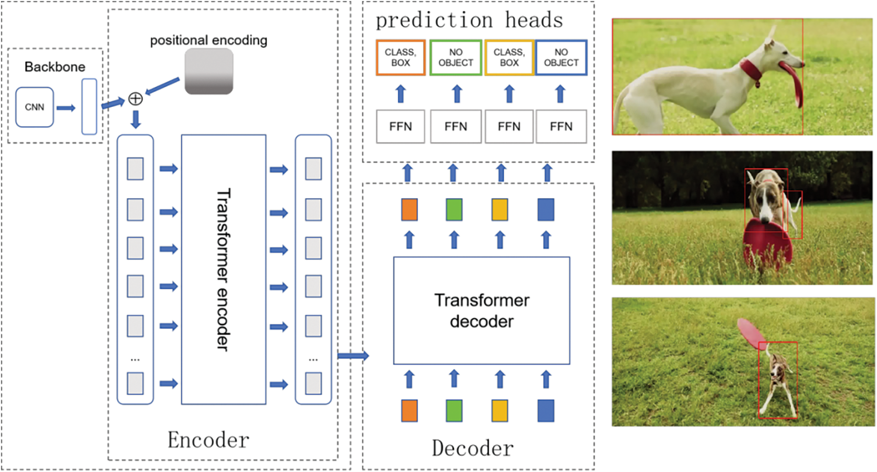
Figure 4: The DETR network architecture
In the DETR network, the feature map of an image, extracted using a CNN backbone, is fed into the Encoder-Decoder architecture based on the Transformer structure. This network transforms the input feature map x into a set of object query features. In the prediction layer, a feedforward neural network (FFN) comprising three linear layers with ReLU (Rectified Linear Unit) activation functions and a hidden layer is used as the detection head. This FFN serves as the regression branch, predicting bounding box coordinates, which encode the normalized center coordinates, height, and width. The predicted class label is then activated using the softmax function.
However, the initialization of the DETR attention module is sparse, leading to prolonged learning periods and slow convergence, which typically results in extensive training. Additionally, the computation demand escalates significantly when detecting high-resolution images. This is mainly due to the Transformer module’s requirement to calculate similarities between each position and every other, unlike the shared parameters in convolutions that entail frequent computations. Deformable DETR integrates deformable convolution from DCN (Deformable Convolution Networks) into DETR to address these challenges. This integration replaces the self-attention in the Encoder and cross-attention in the Decoder, allowing the attention module to focus on a limited number of crucial sampling points surrounding a target. This enhancement enables DETR to deliver improved performance, particularly in detecting smaller targets.
He et al. [32] built upon the foundations laid by DETR and Deformable DETR, we have developed TransVOD, a target detector specifically designed for video applications. TransVOD is an end-to-end object detection system operating on the spatial-temporal Transformer framework. As depicted in Fig. 5, the TransVOD takes multiple frames as input for a given current frame and directly generates the detection results for that current frame through its architectural design.
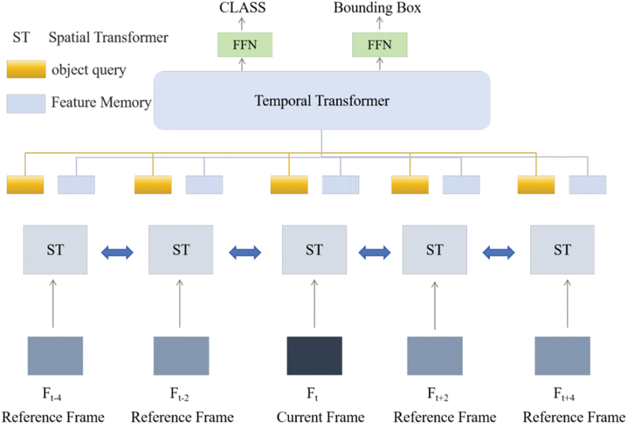
Figure 5: The original TransVOD network
TransVOD is structured around four principal components, each critical in video object detection. Firstly, the Spatial Transformer is employed for single-frame object detection. It extracts object queries and compresses feature representations, creating a memory for each frame. Secondly, the Temporal Deformable Transformer Encoder (TDTE) is integrated. This component fuses with the memory outputs from the Spatial Transformer, thereby enhancing the memory with temporal context.
Thirdly, the Temporal Query Encoder (TQE) links objects from each frame along the time dimension. This linking process is crucial for understanding the temporal dynamics of objects across different frames. Lastly, the Temporal Deformable Transformer Decoder (TDTD) is used to derive the final prediction results for the current frame.
The network architecture of TransVOD, as illustrated in Fig. 6, begins with a CNN backbone that extracts features from multiple frames. These features are then processed through several shared Spatial Transformer Encoders (STE), with the encoded feature memory subsequently relayed to the TDTE. This provides essential location cues for the final Decoder’s output. The TDTE’s key innovation lies in its focus on several pivotal sampling points around a reference point, enabling more efficient feature aggregation across different frames. Concurrently, the Spatial Transformer Decoder (STD) decodes the spatial object query.
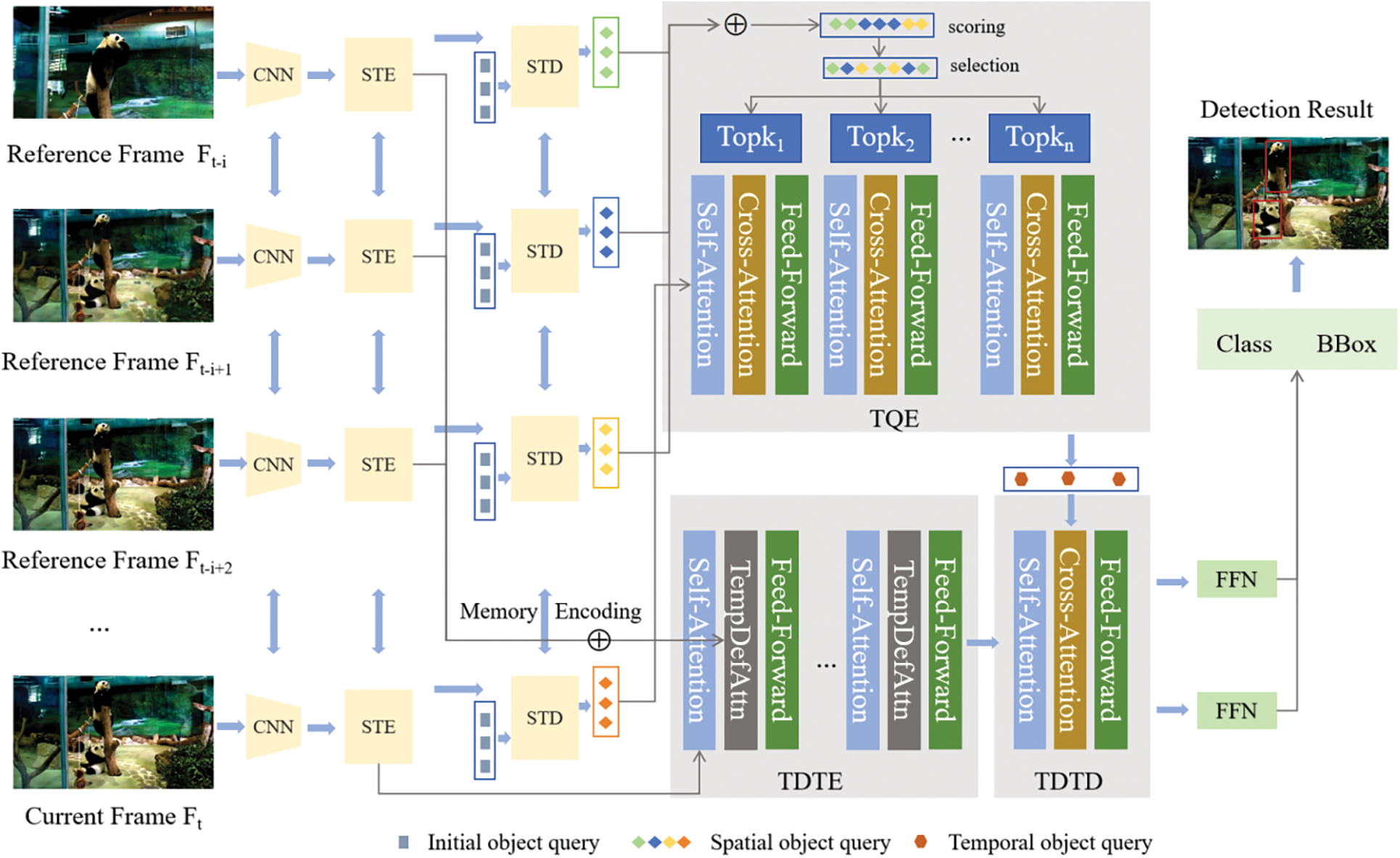
Figure 6: The network of the TransVOD
On the other hand, the TQE connects the Spatial Object Queries from each frame through a temporal Transformer. This process aggregates these queries, learning the temporal context across frames and modeling the interrelationships between different queries. The outputs from the TDTE and TQE feed into the TDTD, which assimilates the temporal context from different frames to predict the final output for the current frame accurately.
The original DETR avoids post-processing and employs a single one-to-one labeling rule to match the STD/TDTD predictions with the actual value using the Hungaria algorithm. Thus, the training process of the Spatial Transformer is consistent with the original DETR. The temporal transformer Uses a similar loss function to predict the target box and category of the two FFN outputs, and the loss function is as follows:
When people watch the video, they only focus on the ROI area, so the overall effect of video enhancement in other areas could be better. In order to improve the speed of model inference and realize the optimization of computation quantity, we hope that the model can enhance the video only for the ROI region.
The RSTT provides us with a perfect backbone. Through the Encoder and Decoder of the transformer, we realize the modeling of temporal and spatial relations. The modeling information can be used both to realize the ROI region identification of video or to do SR.
In Fig. 7, we propose a new loss function, combining the ROI loss function proposed in TransVOD and the loss function of SR proposed in RSTT, to reconstruct the loss function as follows:
where, for the loss of the whole graph, for the loss of the ROI, take the constant of 0.5. Through the loss function of ROI, first guide the attention of the model to the ROI area, and then in the identified ROI area for SR enhancement, we do under the number of different RSTT backbone models, proved that the new loss function, not only can bring better SR effect, to some extent, alleviate the image is too smooth, and can reduce the overall number of the model by 15%, the speed of model inference increased by 10%.
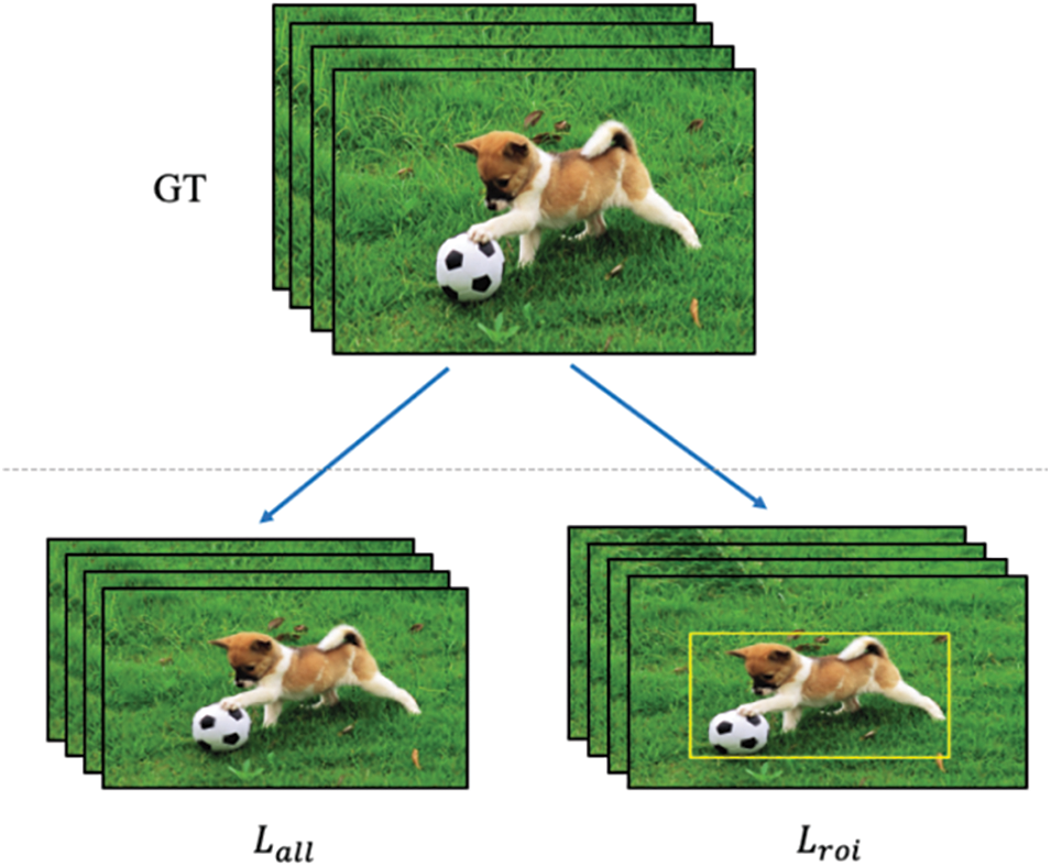
Figure 7: The ROI_Loss guide
The ImageNet VID [33] dataset is a large-scale benchmark dataset in video target detection. It contains 3862 training videos, 555 verification videos, 937 test videos, and the target object boundary box information XML file in the video, which contains 30 basic categories, such as aircraft, antelope, bear bicycle, and motorcycle.
In order to make the format of the ROI region loss boot of the dataset consistent, we modified the dataset based on ImageNet VID. In RSTT training, the whole picture should be randomly cut to the set size and sent to the network, so the data size during training should be uniform. We first took the videos in the training set one by one, output the image size of the video frames larger than seven frames, and recorded the video with the image size of 1920 × 1080 to sep_train list. The txt file is used for partitioning the training set data.
Read the sep_train list. In the text file, all the videos recorded in the file are downsampled to obtain the low-resolution images and their lmdb format data, which are saved separately to generate training set files. The training set file consists of 82 HR images and LR images with the size of 1920 × 1080 videos and their corresponding XML annotation files. Then, read the video with a data set frame number of more than seven and a resolution of 1280 × 720, and save the original video and the downsampled video to generate a test set, which consists of 138 HR images and LR images with the size of 1280 × 720 videos.
When reading the dataset video frame, the box bounding box region corresponding to the frame image is loaded simultaneously. Depending on the data type, the high-resolution image is read from the LMDB database or file system, and the data set XML file is resolved to read the bounding box information of the corresponding frame image. Because RSTT training needs to cut pictures into multiple blocks of the same size in the network training, the box area must also be transformed. After the image is randomly cut, the cropped image and the cut bounding box list are transformed according to the cropped position and the position of the original box.
When loading the data, in order to improve the model performance, we rotated the image, flipped it, and performed other data enhancement operations to increase the diversity of the data set. At the same time, we need to increase the corresponding image box transformation and the corresponding box adjustment to ensure that they are correct in the image position and size.
For the subsequent calculation of loss for convenience, we also need to generate the mask of the ROI region. According to the box boundary box of the video frame image ROI, we set the region setting 0 within the box and the box outside to 1 to generate a mask, extend the generated mask, and copy it to three channels to align with the image. In the subsequent loss of the ROI area, we only need to multiply the predicted image and the original image by the ROI_mask to calculate the loss.
We implemented ROI recognition at the edge, compared to method proposed in which first recognizes the ROI at the cloud server side and then transmits video content at different compression ratios, our newly proposed computation allocation protocol can achieve two benefits: First, it reduces the amount of computation at the cloud server side, which can further reduce processing latency on the cloud server side. Although it increases the amount of computation at the edge side, because of our designed end-to-end ROI and SR unified network, the overall amount of computation in the process is actually reduced. According to our performance tests, the overall computational latency is reduced by 10%. Second, since ROI recognition and super-resolution are allocated to the edge side, the cloud server side can lower the overall resolution of the gaming video to the minimum. Compared to method FRSR (Foveated Rendering Super Resolution) [34], this can save up to 15% in bandwidth, this is affected by the size of the ROI region. According to our subjective experiments, under the condition of not affecting user experience, the transmission bandwidth saved is about 10%–15%.
The testbed for our computer graphics project utilized four devices configured as depicted in Fig. 8: An advanced desktop computer (Intel i7 CPU, RTX 3090 GPU) functioned as the central cloud server, while a less powerful desktop (Intel i5 CPU, RTX 3060 GPU) acted as the edge server. To represent an end-user client device, we used a basic laptop (Intel i3 CPU, integrated graphics). Lastly, an additional laptop was incorporated to provide network connectivity between the cloud and edge machines. In our simulation environment, the end-to-end delay is 100~200 ms, that is 10% improvement compared with method FRSR in the same simulation setting.
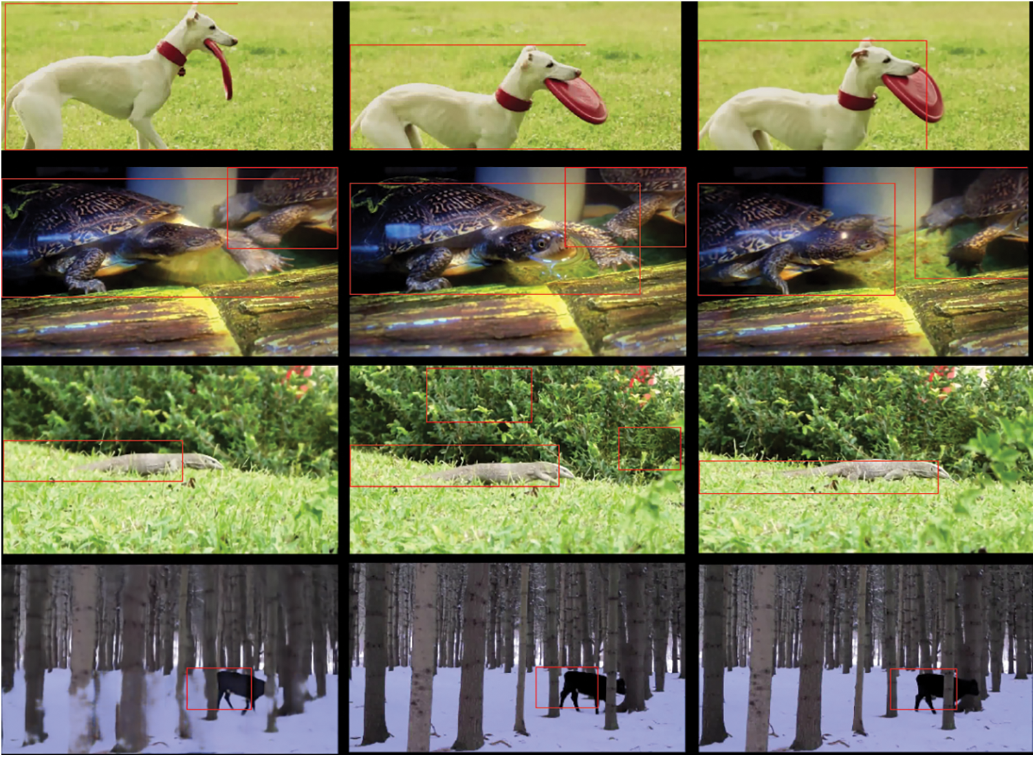
Figure 8: Some functions of x
Pytorch was deployed to implement all the trainings. We explicitly modeled the ROI of the video frame of the training set and detected the ROI region in the LR video frame. During training, the image was randomly cut into multiple 256,256 blocks, and the box size was changed. Meanwhile, we also cut the HR picture of the corresponding area to calculate the reconstruction loss. In addition, the random rotation of 90°, 180°, and horizontal flipping to increase the model’s generalization ability can help the model detect more targets.
As Fig. 9 shows, during the training phase, several key parameters were carefully selected to optimize the learning process and achieve the desired outcomes. The choice of a batch size of 8 was determined based on considerations of computational efficiency and model stability. A batch size of 8 strikes a balance between utilizing parallel processing capabilities and ensuring that the model receives a diverse set of samples in each iteration.
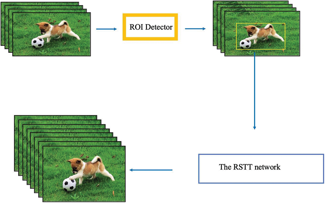
Figure 9: The training details
The decision to run the training for a total of 150,000 epochs was driven by empirical experimentation and iterative model refinement. Extensive testing revealed that this number of epochs allowed the model to converge to a stable state and attain satisfactory performance on the given task. Additionally, monitoring training curves and validation metrics supported the choice of this epoch count as an optimal point for achieving convergence.
The introduction of a newly defined hyperparameter, alpha, set to 0.5, serves the purpose of controlling the proportion of ROI (Region of Interest) loss during training. This choice was motivated by the need to strike a balance between emphasizing the importance of regions containing critical information and maintaining a fair contribution from non-ROI areas. The value of 0.5 for alpha was found to be optimal through sensitivity analysis and experimentation, ensuring that the model gives appropriate consideration to both ROI and non-ROI regions in the learning process.
These parameter settings were fine-tuned through a systematic process of experimentation and evaluation, aiming to achieve optimal model performance while addressing computational constraints and maintaining a balanced consideration of key regions in the input data.
Experiments on the GPU using the Adam optimizer to optimize the network, thus minimizing the loss value of the network training. The initial learning rate was set to 210 (−4). Using a significant learning rate swings the weight gradient back and forth. Reconstruction loss during training does not reach the global minimum. Using the cosine annealing learning rate function to gradually reduce the learning rate, the learning rate is reset to the initial learning rate at the end of each cycle; when the learning rate reaches at 400000, 800000, 1200000 and 1600000 iterations. Also, at each restart point, learning rates will all be reset to half of the initial learning rate, this calculation method helps us to approach the global optimum gradually.
In selecting experimental evaluation indicators, we compare the performance of the test set images and the images under different methods and parameter Settings on the Y channel. Peak signal-to-noise ratio (PSNR) (unit: DB) and structural similarity (Structure Similarity, SSIM [35]) are two indicators commonly used to evaluate this performance quantitatively.
PSNR measures the image reconstruction quality by calculating the error between the corresponding pixels, and the higher value of the peak SNR indicates the smaller the image distortion, i.e., the reconstructed image is more similar to the original high-resolution image. SSIM comprehensively measures the similarity of images from three perspectives: Brightness, contrast, and structure.
(1) PSNR
PSNR is an engineering term that expresses the ratio of the maximum possible power of a signal to the power of destructive noise that affects the accuracy of its representation. Because many signs have a wide dynamic range, the peak signal-to-noise ratio is expressed in logarithmic decibel units.
To calculate PSNR, we must know the value of MSE (Mean Squared Error) first. Two m × n monochrome images I and K, if one is a noisy approximation of the other, then their mean square error is defined as:
When the difference between the real value y and the predicted value f (x) is greater than 1, the error will be amplified; When the difference is less than 1, the error will be reduced, which is determined by the square operation. MSE will give a larger punishment for larger errors (>1), and a smaller punishment for smaller errors (<1). The concept of MSE is well known, which is also a common loss function. And PSNR is obtained by MSE, the formula is as follows:
MAXI is the maximum value that represents the color of the image point. If each sampling point is represented by 8 bits, then it is 255. The numerator in log is the maximum value representing the color of image points. If each sampling point is represented by 8 bits, it is 255. The larger the PSNR, the better the image quality.
(2) SSIM
The image quality assessment, the effect of local calculation of the SSIM index is better than global. First, the statistical features of the image are usually unevenly distributed in space; second, the distortion of the image also varies in length; third, within an average viewing distance, people can only focus on one area of the picture, so the local processing is more in line with the characteristics of the human visual system; fourth, the local quality detection can obtain the mapping matrix of the spatial quality change of the picture, and the result can be used in other applications.
In formula (7), µx and µy represent the average value of x and y, respectively. σx and σy represent the standard deviation of x and y, respectively. σxy represent the covariance of x and y. c1 and c2 are constants respectively to avoid system errors caused by 0 denominator.
4.4 Compared with the Effect of Doing SR
We downsampled the frame images of the videos in the data set, obtained the LR images, performed the super-resolution reconstruction of the LR images, and applied our method to the LR images, which can get the visual qualitative contrast of the low-resolution images only SR and the effect of our method. We selected 138 animal videos moving in front of the stationary camera. We extracted the fifth frame image of the crocodile crawling video as an example, and the contrast effect is shown in Fig. 10.
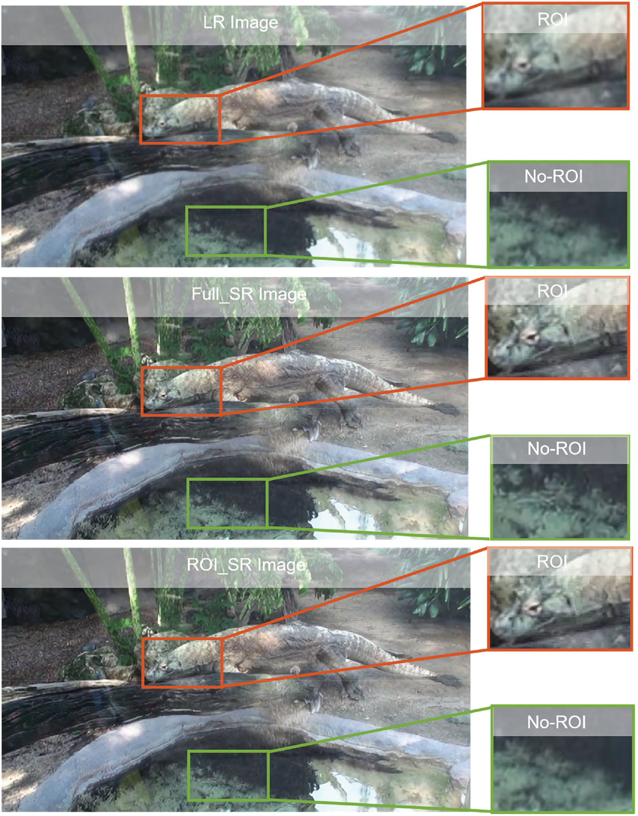
Figure 10: The contrast effect
It can be seen that compared to the whole LR image SR operation, our method when applied to the frame image, image intercepts the interest area clearly than the original LR and restores more texture details and edge contour, but the non-interest area did not do super processing, so the interest area still fuzzy and artifacts, reflected in the figure can see more clear crocodile skin texture. However, when observing the overall effect of the image through the human eye, because the human eye will pay more attention to the crocodile area when observing the image, the observation effect of the human eye is not much different from the image effect after direct SR operation on the whole image.
We also used subjective quality evaluation to measure model quality to analyze the end-to-end performance of our model, especially the user’s perception of the visual quality and smoothness of video frames and whether there was any delay in application, etc. We chose two live broadcasts of different natures, game broadcasting and shopping broadcasting, which are provided to the client through the Internet. To avoid server overload, we only allow one client to connect to the server and control each live broadcast time within 30 min. We invited 10 participants with an age distribution ranging from 20 to 50 years. Each participant watches two live videos in the experiment, in which the original video is played 10 min before the live game, the video of the RSTT model in the first 10 to 20 min, and the video after the ROI in the next 10 min; the video after the ROI in the first 10 min, the video of the RSTT model in the next 10 to 20 min, and the original video in the next 10 min. Participants will be kept from the handling of the live video. At each live broadcast, participants need to score the effect of the live video every 5 min and score from 1 to 5 according to ACR (Absolute Category Rating). One indicates that the live video is naughty, and there is a lot of damage, blur, and lag. A score of 5 indicates the quality of live video without any noticeable lag or distortion.
Table 1 summarizes our mean opinion score (MOS) from the 10 participants. The results showed that the ROI overscore-based model significantly improved the perceived quality of participants in all scenarios. For example, for the live game, RSTT after live video and introducing ROI model after the video effect are significantly higher than the original video MOS 3.1 (average), at the same time because the RSTT model in real-time video processing consumption, causing some live video lag, so our method will MOS from using RSTT model of 3.9 (good) to 4.3 (very good). The MOS also reached 4.4 in our model (perfect). The improvement in inference efficiency brought about by the new method is mainly due to the guidance of ROI_loss. To test our idea, we performed the ablation experiments.

The experimental design performed super-resolution reconstruction of the test images using a benchmark model without introducing ROI_loss and an ROI_loss-guided model, respectively. We evaluated the effect of the new method by calculating the PSNR, PSNR-Y, SSIM, and SSIM-Y values between the processed images and the original images. The evaluation indicators are considered higher values to indicate better results. Tables 2 and 3 below show the index comparison of the whole map region and the ROI region between the benchmark model and the ROI_loss guided model, respectively.


Looking at the data in the table, we can find that the Los-guided model is higher than the benchmark model in the whole map area and ROI area, which indicates that the Los-guided method has some advantages in noise suppression, brightness information retention, and image structure. The ROI-guided model can focus more on the ROI region of the image, which can reduce the redundant computation and processing of non-ROI regions, thus improving the inference efficiency while being reflected in metrics such as PSNR and SSIM. Fig. 11 shows the effect comparison diagram of the ablation experiment.
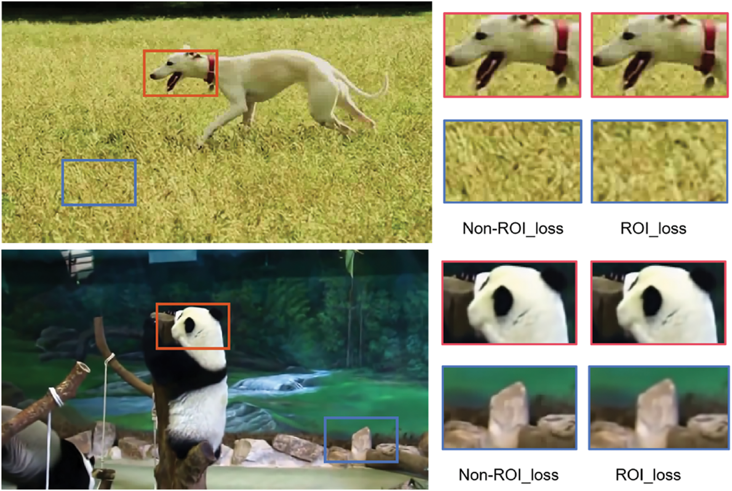
Figure 11: The effect comparison diagram of the ablation experiment
The model’s advantages in this paper must be addressed, but simultaneously, the model still has relative limitations, such as long training time. As with other Transformer-based methods, the training time required for the RSTT is relatively long. Two Nvidia Quadro RTX 6000 cards will take more than 25 days to converge. Meanwhile, the RSTT lacks the flexibility to interpolate at arbitrary timestamps. Unlike TMNet, the model needs more flexibility to interpolate intermediate frames within arbitrary timestamps because the query Q defined in RSTT is fixed. However, a deep study of the model can be achieved by slightly rewriting the query Q of the decoder D3. We only need to query if we want to interpolate n-1 frames between two frames, such as E3, 2t − 1 and E3, 2t + 1. In this way, the flexibility of RSTT model interpolation at arbitrary timestamps.
We define a new video-related task: To identify the region of interest in the video and achieve overdivision for the region of interest to compress the video transmission bandwidth and improve the video enhancement efficiency without affecting the user’s perception. We modified the data set adapted to this new task based on the image video. We combined two state-of-the-art transformer models of video object detection and video hypersegmentation. We realized a new unified model that can complete both tasks at the same time, achieving the optimal ratio of bandwidth compression and video enhancement efficiency. In future, we consider to integrate temporal and spatial information for joint spatiotemporal modeling. By designing models capable of simultaneously capturing inter-frame relationships and spatial features, enhance super-resolution effects in a more comprehensive manner. This involves a deep understanding of spatiotemporal characteristics and appropriate model design.
Acknowledgement: Not applicable.
Funding Statement: This research was funded by National Key Research and Development Program of China (No. 2022YFC3302103).
Author Contributions: Conceptualization, Ying Xu; methodology, Bo Peng; validation, Xinkun Tang, Feng Ouyang; formal analysis, Xinkun Tang; investigation, Ying Xu; resources, Feng Ouyang; writing—original draft preparation, Ying Xu; writing—review and editing, Xinkun Tang; visualization, Feng Ouyang; All authors have read and agreed to the published version of the manuscript.
Availability of Data and Materials: Not applicable.
Conflicts of Interest: The authors declare that they have no conflicts of interest to report regarding the present study.
References
1. C. M. Jia et al., “Video processing and compression technology,” Chinese J. Image Grap., vol. 26, no. 6, pp. 1179–1200, 2021. [Google Scholar]
2. L. Itti, C. Koch, and E. Niebur, “A model of saliency-based visual attention for rapid scene analysis,” IEEE Trans. Pattern Anal. Mach. Intell., vol. 20, no. 11, pp. 1254–1259, Nov. 1998. doi: 10.1109/34.730558. [Google Scholar] [CrossRef]
3. J. Harel, C. Koch, and P. Perona, “Graph-based visual saliency,” in Proc. Adv. Neural Inf. Process. Syst. 19, Vancouver, Canada, 2016, pp. 44–51. [Google Scholar]
4. D. S. Cruz et al., “Region of interest coding in JPEG2000 for interactive client/server applications,” in Proc. IEEE Third Workshop Multimed. Signal Process., 1999, pp. 389–394. [Google Scholar]
5. B. E. Usevitc, “A tutorial on modern lossy wavelet inmages compression: Foundations of JPEG 2000,” IEEE Signal Proc. Mag., vol. 187, no. 5, pp. 22–35, 2001. [Google Scholar]
6. J. C. Huang and Y. Wang, “Compression of color facial image using feature correction two-stage vector quantization,” IEEE Trans. Image Process., vol. 8, no. 1, pp. 102–109, 1999. [Google Scholar] [PubMed]
7. W. Bao et al., “Depthaware video frame interpolation,” in Proc. 2019 IEEE/CVF Conf. Comput. Vision Pattern Recognit. (CVPR), Long Beach, CA, USA, 2019, pp. 3703–3712. [Google Scholar]
8. M. Park, H. G. Kim, S. Lee, and Y. M. Ro, “Robust video frame interpolation with exceptional motion map,” IEEE Trans. Circ. Syst. Vid. Teach., vol. 31, no. 2, pp. 754–764, Feb. 2021. doi: 10.1109/TCSVT.2020.2981964. [Google Scholar] [CrossRef]
9. S. Meyer, O. Wang, H. Zimmer, M. Grosse, and A. Sorkine-Hornung, “Phase-based frame interpolation for video,” in Proc. 2015 IEEE Conf. Comput. Vision Pattern Recognit. (CVPR), Boston, MA, USA, 2015, pp. 1410–1418. [Google Scholar]
10. Z. Liu, R. A. Yeh, X. Liu, Y. Liu, and A. Agarwalac, “Video frame synthesis using deep voxel flow,” in Proc. IEEE Int. Conf. Comput. Vision, Venice, Italy, 2017, pp. 4463–4471. [Google Scholar]
11. S. SloMo, “High quality estimation of multiple intermediate frames for video interpolation,” in Proc. IEEE Conf. Comput. Vision Pattern Recognit., Salt Lake City, UT, USA, 2018. [Google Scholar]
12. D. B. de Jong, F. Paredes-Vallés, and G. C. H. E. de Croon, “How do neural networks estimate optical flow? A neuropsychology-inspired study,” IEEE Trans. Pattern Anal. Mach. Intell., vol. 44, no. 11, pp. 8290–8305, Nov. 1, 2022. doi: 10.1109/TPAMI.2021.3083538. [Google Scholar] [PubMed] [CrossRef]
13. S. Niklaus, L. Mai, and F. Liu, “Video frame interpolation via adaptive convolution,” in Proc. IEEE Conf. Comput. Vision Pattern Recognit., Honolulu, HI, USA, 2017, pp. 670–6794. [Google Scholar]
14. S. Oprea et al., “A review on deep learning techniques for video prediction,” IEEE Trans. Pattern Anal. Mach. Intell., vol. 44, no. 6, pp. 2806–2826, Jun. 1, 2022. doi: 10.1109/TPAMI.2020.3045007. [Google Scholar] [PubMed] [CrossRef]
15. Y. Han, G. Huang, S. Song, L. Yang, H. Wang and Y. Wang, “Dynamic neural networks: A survey,” IEEE Trans. Pattern Anal. Mach. Intell., vol. 44, no. 11, pp. 7436–7456, Nov. 1, 2022. doi: 10.1109/TPAMI.2021.3117837. [Google Scholar] [PubMed] [CrossRef]
16. S. Xiang and B. Tang, “Kernel-based edge-preserving methods for abrupt change detection,” IEEE Signal Process. Letters, vol. 27, pp. 86–90, 2020. doi: 10.1109/LSP.2019.2957645. [Google Scholar] [CrossRef]
17. F. Harrou, A. Saidi, Y. Sun, and S. Khadraoui, “Monitoring of photovoltaic systems using improved kernel-based learning schemes,” IEEE J. Photovolt., vol. 11, no. 3, pp. 806–818, May 2021. doi: 10.1109/JPHOTOV.2021.3057169. [Google Scholar] [CrossRef]
18. X. Cheng and Z. Chen, “Multiple video frame interpolation via enhanced deformable separable convolution,” IEEE Trans. Pattern Anal. Mach. Intell., vol. 44, no. 10, pp. 7029–7045, Oct. 1, 2022. doi: 10.1109/TPAMI.2021.3100714. [Google Scholar] [PubMed] [CrossRef]
19. L. Deng, M. Yang, H. Li, T. Li, B. Hu and C. Wang, “Restricted deformable convolution-based road scene semantic segmentation using surround view cameras,” IEEE Trans. Intell. Transport. Syst., vol. 21, no. 10, pp. 4350–4362, Oct. 2020. doi: 10.1109/TITS.2019.2939832. [Google Scholar] [CrossRef]
20. H. Lee, T. Kim, T. Chung, D. Pak, Y. Ban and S. Lee, “Adaptive collaboration of flows for video frame interpolation,” in Proc. IEEE/CVF Conf. Comput. Vision Pattern Recognit., Seattle, WA, USA, 2020, pp. 5316–5325. [Google Scholar]
21. H. Liu et al., “Video super resolution based on deep learning: A comprehensive survey,” arXiv preprint arXiv:2007.12928, 2020. [Google Scholar]
22. J. Dai et al., “Deformable convolutional networks,” in Proc. IEEE Int. Conf. Comput. Vision, Venice, Italy, 2017, pp. 764–773. [Google Scholar]
23. Y. P. Tian, Y. L. Zhang, Y. Fu, and C. Xu, “TDAN: Temporally-deformable alignment network for video super-resolution,” in Proc. 2020 IEEE/CVF Conf. Comput. Vision Pattern Recognit. (CVPR), Seattle, WA, USA, 2020, pp. 3357–3366. [Google Scholar]
24. X. Wang, K. C. K. Chan, K. Yu, C. Dong, and C. C. Loy, “EDVR: Video restoration with enhanced deformable convolutional networks,” in Proc. IEEE Conf. Comput. Vision Pattern Recognit. Workshops (CVPRW), Long Beach, CA, USA, 2019. [Google Scholar]
25. M. Lu and P. Zhang, “Grouped spatio-temporal alignment network for video super-resolution,” IEEE Signal Process. Letters, vol. 29, pp. 2193–2197, 2022. doi: 10.1109/LSP.2022.3210874. [Google Scholar] [CrossRef]
26. E. Shechtman, Y. Caspi, and M. Irani, “Increasing space-time resolution in video,” in Proc. European Conf. Comput. Visio, Copenhagen, Denmark, 2002, pp. 753–768. [Google Scholar]
27. M. Haris, G. Shakhnarovich, and N. Ukita, “Space-time-aware multi-resolution video enhancement,” in Proc. IEEE Conf. Comput. Vision Pattern Recognit. (CVPR), Seattle, WA, USA, 2020, pp. 2859–2868. [Google Scholar]
28. X. Y. Xiang et al., “Zooming Slow-Mo: Fast and accurate one-stage space-time video super-resolution,” in Proc. IEEE/CVF Conf. Comput. Vision Pattern Recognit. (CVPR), Seattle, WA, USA, 2020, pp. 3370–3379. [Google Scholar]
29. G. Xu et al., “Temporal modulation network for controllable space-time video super-resolution,” in Proc. IEEE/CVF Conf. Comput. Vision Pattern Recogniti. (CVPR), New Orleans, LA, USA, 2021, pp. 6388–6397. [Google Scholar]
30. Z. C. Geng et al., “RSTT: Real-time spatial temporal transformer for space-time video super-resolution,” in Proc. 2022 IEEE/CVF Conf. Comput. Vision Pattern Recognit. (CVPR2022, New Orleans, LA, USA, 2022, pp. 17441–17451. [Google Scholar]
31. X. Z. Zhu et al., “Deformable DETR: Deformable transformers for end-to-end object detection,” arXiv preprint arXiv:2010.04159, 2020. [Google Scholar]
32. L. He et al., “TransVOD: End-to-end video object detection with spatial-temporal transformers,” IEEE Trans. Pattern Anal. Mach. Intell., vol. 45, no. 6, pp. 7853–7869, 2022. doi: 10.1109/TPAMI.2022.3223955. [Google Scholar] [PubMed] [CrossRef]
33. O. Russakovsky et al., “ImageNet large scale visual recognition challenge,” Int. J. Comput. Vision, vol. 115, no. 3, pp. 211–252, 2015. [Google Scholar]
34. X. K. Tang, Y. Xu, F. Ouyang, L. Zhu, and B. Peng, “A cloud-edge collaborative gaming framework using AI-powered foveated rendering and super resolution,” Int. J. Semant. Web Inf., vol. 19, no. 1, pp. 1–19, 2023. doi: 10.4018/IJSWIS. [Google Scholar] [CrossRef]
35. Z. Wang, A. C. Bovik, H. R. Sheikh, and E. P. Simoncelli, “Image quality assessment: From error visibility to structural similarity,” IEEE Trans. Image Process., vol. 13, no. 4, pp. 600–612, 2004. doi: 10.1109/TIP.2003.819861. [Google Scholar] [PubMed] [CrossRef]
Cite This Article
 Copyright © 2024 The Author(s). Published by Tech Science Press.
This work is licensed under a Creative Commons Attribution 4.0 International License , which permits unrestricted use, distribution, and reproduction in any medium, provided the original work is properly cited.
 Downloads
 Citation Tools