Fault Diagnosis Scheme for Railway Switch Machine Using Multi-Sensor Fusion Tensor Machine

1  Introduction

Urban rail transit (URT) has become an essential means of transportation due to the swift urbanization encountered by numerous nations. By the end of 2023, China’s URT network has covered over ten thousand kilometers [1]. The increasing attention towards Prognostics and health management (PHM) in railways has been brought about by the expansion of the URT network. Fig. 1 illustrates the relationship between the railway switch machine and the switch & crossing system. The primary function of the railway switch machine is to control track switching and alter the train’s direction [2,3]. However, the railway switch machine is susceptible to damage since it is exposed to harsh weather or wet tunnel conditions. Currently, the maintenance strategy for railway switch machine relies on scheduled time-based maintenance. The condition of the railway switch machine is evaluated by monitoring various signals, including power, current, and force signals. In PHM research, fault diagnosis is a key subject that aids inspectors in determining if a sample is defective and pinpointing the exact nature of the fault. Applying fault diagnosis can help reduce the workload and time costs of the inspector [4,5].

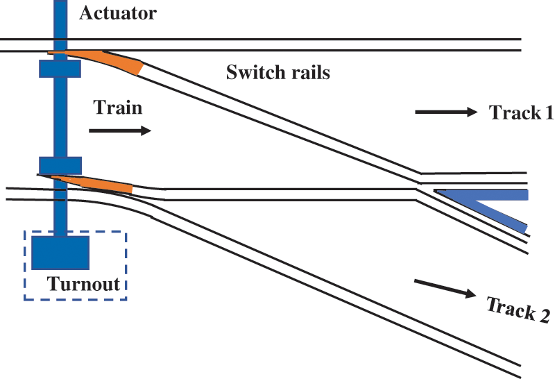
Figure 1: Schematic representation of switch & crossing systems configurations

PHM for railway switch machine has garnered the attention of scholars [6]. The availability of accumulating historical data and the advancement of data acquisition equipment have provided valuable research opportunities [7–9]. Based on the feature extraction of the models, existing research on fault diagnosis for railway switch machine can be categorized into three distinct groups: Recognition with distance measurement, classifier with manual feature, and deep learning with automatic feature. Recognition with distance measurement involves utilizing distance metrics to compare curve distances, thereby facilitating fault diagnosis. A fault diagnosis scheme for railway switch machine was presented using dynamic time warping and Hausdorff distance in [10]. The fault diagnosis scheme was conducted by comparing the current curves using dynamic time warping in [11]. In [12], a method for diagnosing faults in railway turnouts was introduced, which consisted of two stages and utilized the Fréchet distance to detect irregular curve data. This method considers the spatial information of time series data and possesses interpretability. However, this method relies heavily on standard curves, making it less general in real applications.

In the classifier with manual feature method, the primary components of these manually extracted features are predominantly based on statistical or signal processing methods. For example, a fault diagnosis scheme for railway switch machine was developed, utilizing statistical characteristics and support vector machine (SVM) in [13]. In [14], a method for diagnosing faults in the high-speed rail switch machine utilizing wavelet packets was introduced. The feature of this approach is determined by the energy entropy of the wavelet packet. In [15], the fault diagnosis method for the high-speed rail switch machine with Extreme Learning Machine was employed using a neural network-based approach. This study employs segmental statistical features extracted from power data in the time domain. The work in [16] introduces a pioneering sound signal-based method to evaluate the degradation status of ZDJ9 railway turnouts, using signal processing operations and statistical analysis for robust feature extraction. In [17], the study accomplishes railway turnout fault diagnosis through the integration of multi-domain feature extraction and an ensemble feature selection strategy, ultimately utilizing SVM for the diagnostic process. These studies focus solely on extracting local information features from the signal while neglecting the spatial structure and contour details inherent in the original data, thereby limiting both accuracy and interpretability.

In recent years, there has been a significant advancement in the rapid development of deep learning with automatic feature [18]. In [19], a method for diagnosing faults in high-speed rail switch machine was introduced, utilizing a convolutional neural network (CNN). In this method, the one-dimensional current signal is segmented, spliced into two-dimensional (2D) images, and then fed into the CNN model. The work in [20] developed a railway turnout diagnosis method with one-dimensional CNN and power curve data. This method adopts the normalized one-dimensional power signal as the input. A scheme was presented in [21] that addresses the issue of limited labeled fault data by using a dual-scale neural network-based fault diagnosis approach. The input for the method was the vibration signal in one dimension. In [22], a fault diagnosis method for railway switch machine was developed, utilizing an autoencoder-based approach. The method takes one-dimensional power signals as inputs. These methods efficiently alleviate the constraints linked to professional expertise. Nevertheless, the neglect of temporal series data’s structural information in these studies during data processing or modeling leads to the omission of spatial structure-related information, consequently affecting the performance and interpretability of the approach.

In real-world turnout fault diagnosis scenarios, inspectors rely on time series data such as turnout power, current, and rotational force to visually assess the condition of the equipment. The evaluation of railway turnout conditions heavily relies on spatial structure-related information of the time series data in this particular context. In addition, existing studies primarily utilize single-mode data, which cannot comprehensively monitor the turnout’s status [23]. The tensor learning model, which accepts tensors as input, effectively preserves more spatial structural information and is well-suited for developing image-based fault diagnosis models. The flexible convex hull-based tensor machine, a well-known method in tensor learning, exhibits lower computational efficiency. A novel fusion and flexible convex hull-based tensor machine (FFCHTM) is developed to overcome the limitations of existing studies, falling under the classifier category that utilizes the manual feature method. It employs image representations and tensor learning to effectively model and capture spatial structure-related information. Meanwhile, a fusion strategy is integrated into the tensor model, enabling the model to fuse and learn information from multi-mode data. In summary, this study offers the following contributions:

1) this paper proposes a domain knowledge-based fault diagnosis scheme for railway turnout, considering monitoring data’s spatial structure-related information.

2) FFCHTM is designed to take advantage of tensor learning for spatial structure-related information and use sufficient information from multi-mode data.

3) the validation of the suggested approach is conducted using actual datasets collected from subway stations. The results of the experiment show that the suggested approach is an effective framework for implementing the diagnosis of turnout faults.

This paper is organized as follows: Section 2 provides a description of the data used. The developed diagnostic scheme is detailed in Section 3. In Section 4, this scheme is tested using real-field data. Finally, Section 5 concludes the paper with a discussion of future research directions.

2  Data Description

The dataset employed in this research was sourced from the ZDJ9 railway switch machine situated within the operational subway stations. This electronic transmission device consists of three-phase currents (characterized as A, B, and C phase) provided by the 380V three-phase AC power supply. Once the state transitions, the ZDJ9 turnout can be completed within a time frame of 7–9 s, operating at a sample rate of 25 Hz. As noted in the literature [23], inspectors observe the A-, B-, and C-phase currents during on-site inspections to assess the railway turnout’s health condition. Accordingly, this study employs current curves from A-, B-, and C-phase to construct models and ascertain the status of ZDJ9 switches. The railway switch machine’s operation condition is divided into two scenarios: Transition from reverse to normal direction (termed the RN state) and transition from normal to reverse direction (referred to as the NR state). Fig. 2 illustrates the performance of the A-, B-, and C-phase currents under two distinct states when the equipment is functioning normally.

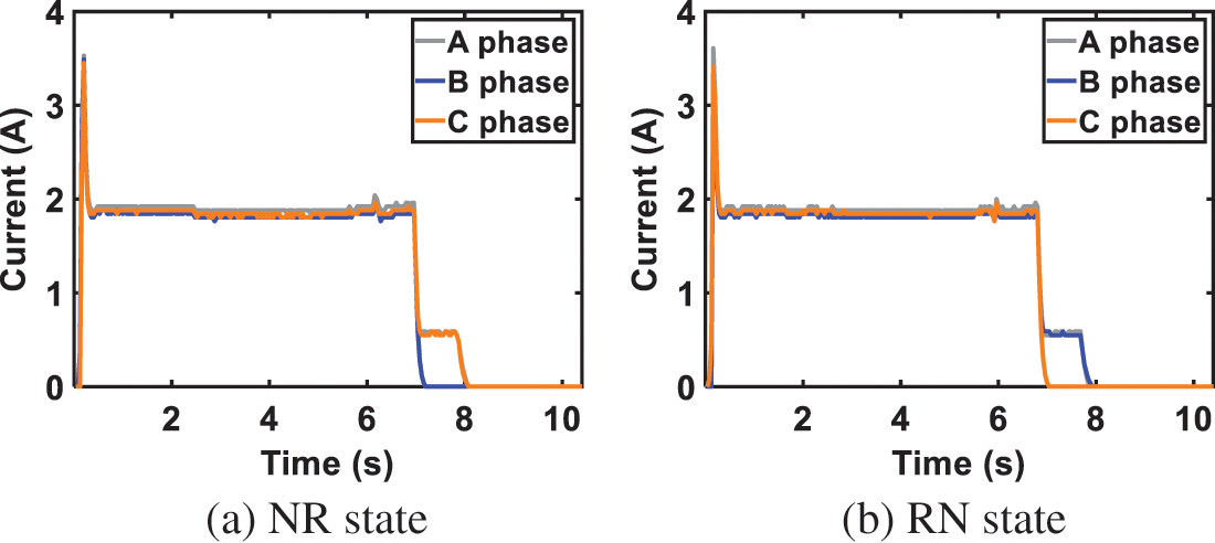
Figure 2: The example of the normal A-, B-, and C- current curves

In standard operating scenarios, the current curves for the A, B, and C phases exhibit four distinct phases: Unlocking, transitioning, locking, and gradual release. Each of these phases is characterized by distinct features, which are detailed below:

•   The motor generates a powerful force to overcome resistance and unlock the switch machine. As a result, the current exhibits a rapid increase, characterized by a prominent pulse peak in the curve. The A-phase, B-phase, and C-phase currents show similar trends in the NR and RN states.

•   Transitioning. During the conversion process, the motor supplies steady power to pull the switch. The current curve remains relatively smooth with slight fluctuations. The A-, B-, and C-phase currents exhibit similar trends in the NR and RN states.

•   Locking. During the locking phase, the electrical current reduces in order to secure the switch in its designated position. Locking is a quick process, and the behavior of the three-phase currents differs in this stage. The A-phase current retains some current value in the RN and NR states. In the NR state, the B-phase current becomes zero, whereas it maintains a certain current value in the RN state. In the NR state, the C-phase current maintains a certain current value, whereas it decreases to zero in the RN state.

•   Gradual release. As the locking process concludes, the current is disconnected. The A-phase current exhibits a slow release in both the RN and NR states. The B-phase current is zero in the NR state and exhibits a slow release in the RN state. The C-phase current experiences a slow release in the NR state and is zero in the RN state.

Table 1 and Fig. 3 depict the nine representative railway turnout states. It is evident that the turnout exhibits different curve shapes under various categories.

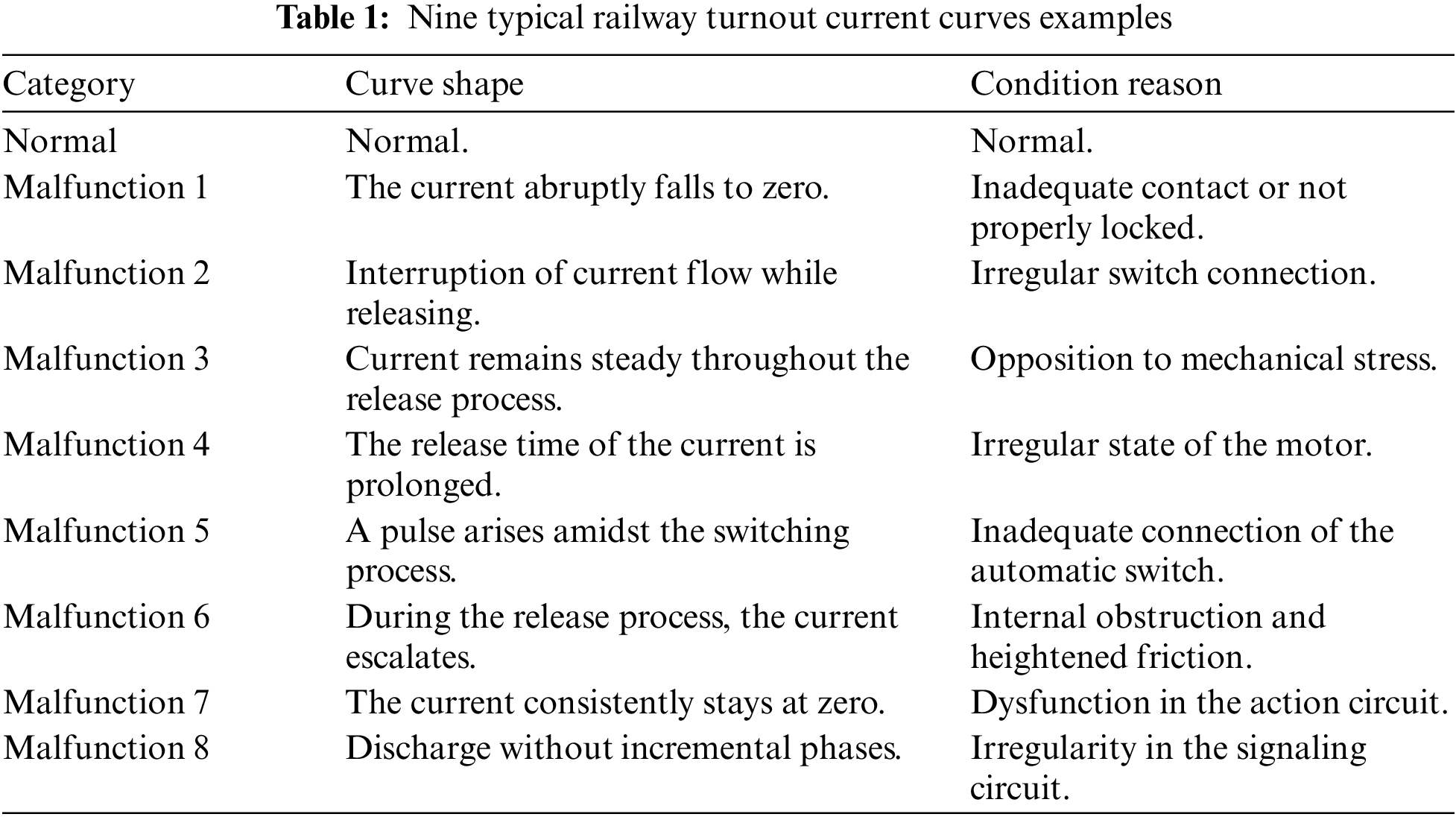
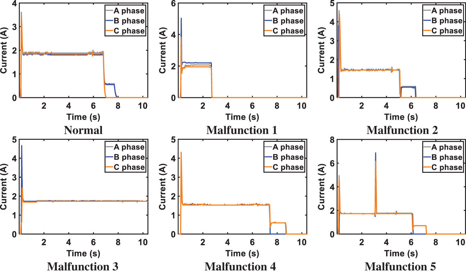
Figure 3: Nine typical railway turnout current curves examples

3  Proposed Diagnosis Scheme

This research introduces a fault diagnosis scheme for railway switch machines, leveraging the three-phase current curve and incorporating the tensor learning machine. Employing current signals from phases A, B, and C as inputs, the scheme systematically classifies the output into either normal data or fault data, with the latter identified by specific fault types. Fig. 4 illustrates the three steps involved in the presented approach: Data preprocessing, fusion feature tensor generation, and tensor-based learning. The specifics of these steps are delineated as follows:

•   Data pre-processing. This step is designed to preprocess the raw curve data, which aligns with the input specifications of the constructed tensor-based model and preserves a significant quantity of spatial structure-related information. The procedure includes the cleansing, standardization, and creation of images based on the existing curve data. Images of a specified size are generated using the MATLAB software.

•   Fusion feature tensor generation. In this module, a fusion strategy is proposed to fuse the information of the three-phase currents to provide sufficient information by multi-representation data. The image representation from the three-phase current is stacked as a three-dimensional tensor. CANDECOMP/PARAFAC (CP) decomposition is adopted to acquire the fusion tensor.

•   Tensor-based learning. The second module calculates the fusion feature tensor, which is then used to conduct tensor machine-based supervised learning in this module. The module consists of two primary components: Building the model and diagnosing faults in test data.

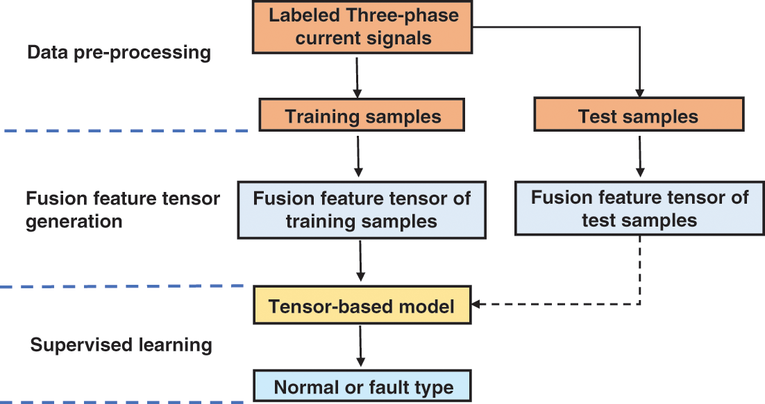
Figure 4: The structure of the developed diagnosis scheme

3.1 Data Pre-Processing

In real-world scenarios, the maintenance scheme for railway switch machine typically involves regular on-site inspections by inspectors. Inspectors rely on visual observation to monitor data images. Inspired by this domain knowledge, this study uses 2D representation for one-dimensional current data to preserve more spatial structure. The effectiveness of using 2D images to represent one-dimensional signal data for modeling has been validated in literature [24]. Unlike the frequency domain representation of vibration signals discussed in that study, our research targets the current data of railway switches, employing a direct conversion into current images. In this context, our proposed data representation method offers advantages over the conventional use of one-dimensional data or 2D time-frequency images as input [25]. The proposed 2D image format is well-suited to the background knowledge required for on-site monitoring and offers a more straightforward implementation, as it bypasses complex signal processing operations. Initially, the data undergoes a cleaning process, which primarily involves the removal of duplicates, irrelevant, and erroneous entries. Subsequently, for standardization purposes, 0–1 normalization is applied to images to boost computational efficiency. Raw current curves are then utilized to create images using MATLAB’s plot functions, and Fig. 5 illustrates this image representation process.

Figure 5: The illustrative blueprint for transforming time series data into image format

3.2 Fusion Feature Tensor Generation

According to Section 2, the present depiction of the ZDJ9 railway point machine encompasses A-phase, B-phase, and C-phase currents, each of which conveys distinct information pertinent to fault diagnostics. A fusion strategy is adopted in this module to integrate the information from the three-phase current. Fig. 6 illustrates the generation of the fusion feature tensor. Firstly, the 2D image is transformed into a three-dimensional tensor through stacking. Next, the stacked tensor undergoes CP decomposition to generate the feature tensor. The three-dimensional tensors are orthogonally decomposed and concatenated in the same direction, resulting in rank-one tensors. The fused feature tensor contains information about the three-phase current and the correlation between them in the physical space. Consequently, the fusion tensor can provide more comprehensive information than single-mode data.

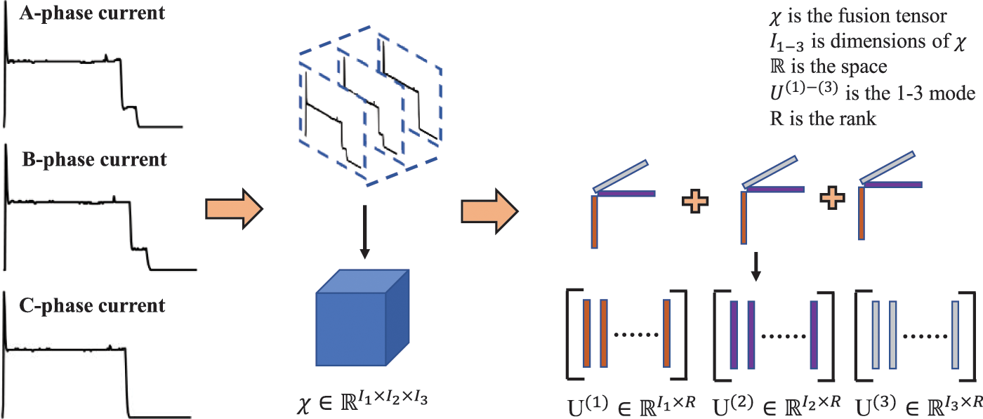
Figure 6: The flowchart of fusion feature tensor generation

3.3 Tensor Learning

The model is constructed using the flexible convex hull-based tensor machine [26,27] in this study. In this work, we have developed a tensor machine called FFCHTM that combines fusion and flexible convex hull techniques.

By defining the tensor dataset, A={Am}m=1k, we can establish the corresponding adaptable representation.

ϕ(A)={∑m=1kεmAm|∑m=1k⁡εm=1,1−βk≤εm≤1−βk+β},(1)

where εi is the combination factor of i-th sample Ai and k represents the sample number of dataset A. β denotes the flexible factors.

For the binary classification case, the flexible convex hull representations for positive and negative samples are as follows:

ϕ(A+)={∑m=1k+⁡ε+mA+m|∑m=1k+⁡ε+m=1,1−β+k+≤ε+m≤1−β+k++β+},(2)

ϕ(A−)={∑m=1k−⁡ε−mA−m|∑m=1k−⁡ε−m=1,1−β−k−≤ε−m≤1−β−k−+β−},(3)

where A+m (m = 1, 2, …, l+) and A−m (m = 1, 2, …, l−) denote the affirmative and opposing tensor samples, correspondingly. The combination factor is ε+m (m = 1, 2, …, l+) and ε−m(m = 1, 2, …, l−). β+ and β− denote the flexible factor, correspondingly. k+ and k− are the number of the A+ and A−.

To discover the optimal separating hyper-plane between ϕ(A_+) and ϕ(A_–) in a linearly separable scenario, the initial step is to locate the closest points between ϕ(A_+) and ϕ(A_–). This can be formulated as the minimum modulus optimization problem [28] in the subsequent manner.

minε+,ε−12||∑m=1k+⁡ε+mA+m−∑m=1k−⁡ε−mA−m||2,(4)

s.t.∑m=1k+⁡ε+m=1,1−β+k+≤ε+m≤1−β+k++β+,m=1,2,…,k+,

s.t.∑m=1k−ε−m=1,1−β−k−≤ε−m≤1−β−k−+β−,m=1,2,…,+ k−.

The function (4) can be expanded as follows:

minε+,ε−12(∑m=1k+∑n=1k+ε+mε+n⟨A+m,A+n⟩+∑m=1k−∑n=1k−ε−mε−n⟨A−m,A−n⟩−2∑m=1k+∑n=1k−ε+mε−n⟨A+m,A−n⟩)(5)

s.t.∑m=1k+ε+m=1,1−β+k+≤ε+m≤1−β+k++β+,m=1,2,…,k+,

s.t.∑m=1k−ε−m=1,1−β−k−≤ε−m≤1−β−k−+β−,m=1,2,…,+ k−.

To solve the function (5), inner tensor product ⟨A+m,A+n⟩, ⟨A−m,A−n⟩ need to be calculated first. For example, the decomposition of the inner tensor product ⟨Am,An⟩ is achieved by utilizing the CP decomposition as described in Section 3.2.

Am=∑P=1Ramp(1)∘amp(2)∘amp(3),(6)

An=∑q=1Ranq(1)∘anq(2)∘anq(3),(7)

where amp(1), amp(2), and amp(3) represent the modes of tensor samples with CP decomposition. R is an integer, and tensor A is a rank-one tensor when R = 1.

Therefore, the inner tensor product ⟨Ai,Aj⟩ can be represented as follows:

⟨Am,An⟩=⟨∑P=1Ramp(1)∘amp(2)∘amp(3),∑q=1Ranq(1)∘anq(2)∘anq(3)⟩=∑p=1R∑q=1R∏n=13⟨amp(n),anq(n)⟩.(8)

The optimization problem stated in Eq. (5) can be converted into:

minε+,ε−12(∑m=1k+∑n=1k+∑p=1R∑q=1Rε+mε+n∏n=13⟨a+mp(N),a+nq(N)⟩+∑m=1k−∑n=1k−∑p=1R∑q=1Rε−mε−n∏N=13⟨a−mp(N),a−nq(N)⟩−2∑m=1k+∑n=1k−∑p=1R∑q=1Rε+mε−n∏N=13⟨a+mp(N),a−nq(N)⟩),(9)

s.t.∑m=1k+ε+n=1,1−β+k+≤ε+m≤1−β+k++β+,m=1,2,…,k+,

s.t.∑m=1k−ε−m=1,1−β−k−≤ε−m≤1−β−k−+β−,m=1,2,…,+k−.

It can be seen that Eq. (9) is a quadratic programming problem, which has the standard optimization solution.

The shrinkage factor [29] is utilized in situations where linearity is not possible. The shrinkage factor is utilized to alter the convex hull’s shape and make it linearly separable. Likewise, Eq. (5) can be converted into:

minε+,ε−12(∑m=1k+∑n=1k+∑p=1R∑q=1Rε+mε+n∏N=13⟨a+mp(N),a+nq(N)⟩+∑m=1k−∑n=1k−∑p=1R∑q=1Rε−mε−n∏N=13⟨a−mp(N),a−nq(N)⟩−2∑m=1k+∑n=1k−∑p=1R∑q=1Rε+mε−n∏N=13⟨a+mp(N),a−nq(N)⟩),(10)

s.t.∑m=1k+ε+m=1,1−β+k+≤ε+m≤1−β+k++β+δ+,m=1,2,…,k+,

s.t.∑m=1k−ε−m=1,1−β−k−≤ε−m≤1−β−k−+β−δ−,m=1,2,…,+k−

where δ+ and δ− are the shrinkage factor. The optimization problem (10) is still a conventional quadratic programming problem, which is resolved utilizing the standard optimization solution.

Suppose that (ε1∗,ε2∗,…,εl∗)T is the optimal solution, and A+∗, A−∗ is the related nearest neighbor points. Next, the optimal hyperplane’s weight tensor W∗ and bias b∗ can be acquired.

W∗=A+∗−A−∗,(11)

b∗=−12WT(A+∗−A−∗).(12)

The decision function is subsequently determined.

F(A)= sign {⟨W∗,A⟩+b∗}.(13)

The decision function will predict the class label of the new tensor sample. To transform the binary FFCHTM into the multi-class FFCHTM, the one-on-one approach [30] is utilized.

4  Experiments and Evaluation

4.1 Experimental Setup

In this study, we leverage in-situ datasets from the ZDJ9 turnout within the metropolitan subway. CASCO, the comprehensive rail transit control system integrator, gathered the data at various stations along Shanghai Metro Line 13. The schemes are implemented using Python. The programming is accomplished on a workstation with an Intel i7-8700 CPU and NVIDIA RTX 2080 GPU. The FFCHTM’s kernel function adopts the Gaussian kernel. The hyperparameters encompassed the kernel parameter σ, adjusted within a spectrum ranging from 0.01 to 600, and the shrinkage factor, set at a value of 0.25. Three evaluation metrics are selected for comparison: Recall, precision, and F1-score. The Macro-averaging strategy is adopted to expand the recall, precision, and F1-scores from the binary classification metrics to multi-class indicators. We employed a five-fold cross-validation approach to determine the best hyper-parameter values across all models within specified ranges. The selection of the optimal parameter set was guided by its effectiveness in reducing the F1-score.

Recall=1l∑j=1lTPjFNj+TPj,(14)

Precision=1l∑j=1lTPjFPj+TPj,(15)

F1−score=1l∑j=1lTPj(FNj+FPj)/2+TPj,(16)

where the j denotes the total number of classes. False Negative, False Positive, and True Positive are represented by FNj, FPj, and TPj, respectively.

4.2 Feature Tensor Effectiveness Analysis

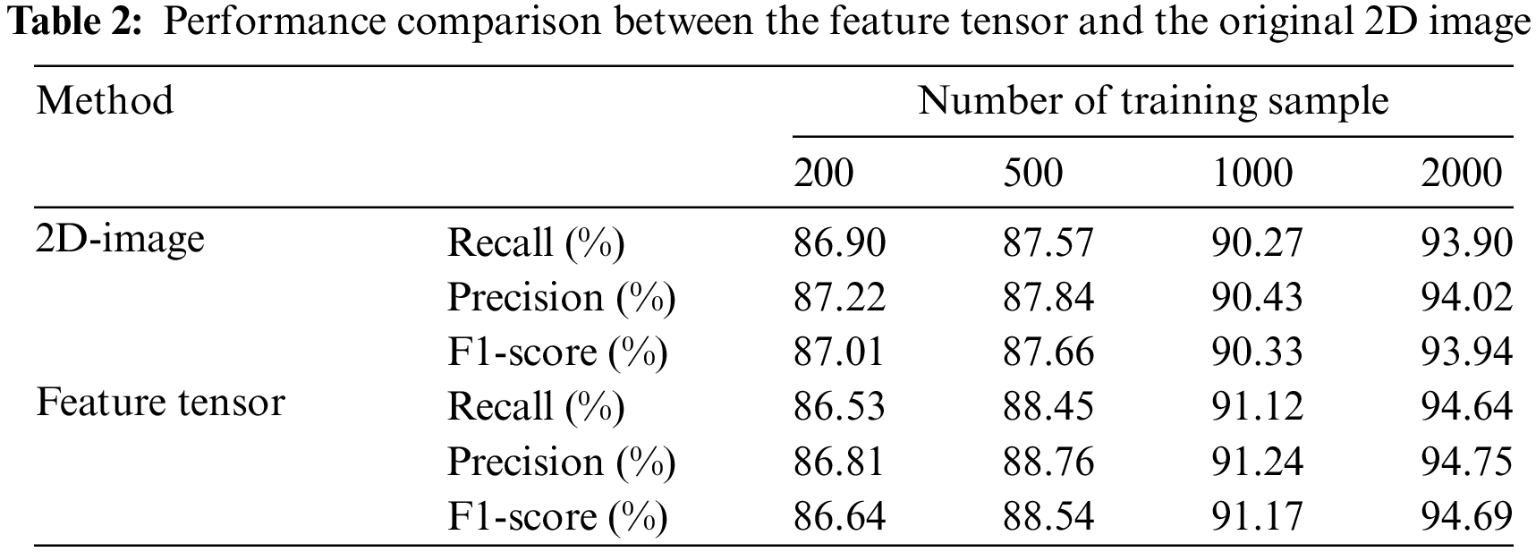
To assess the efficacy of the feature tensor, this subsection presents a comparative analysis between the feature tensor and the original 2D image representation. The original 2D image features are derived by straightforwardly stacking the three-phase current images. Both types of features are modeled using the proposed FFCHTM. Table 2 shows the comparison result and indicates that the feature tensor outperforms the 2D image representation. This enhanced performance can be attributed to the feature tensor’s capability to encapsulate the intricate structural information present within multidimensional data.

4.3 Comparisons with the One-Dimensional Data-Based Method

4.3.1 Comparison Method

To evaluate the efficacy of the proposed method, we undertook a comparative analysis with the fault diagnosis schemes currently documented in the existing literature. First, the comparisons with the one-dimensional data-based method are investigated. The models employed for comparative analysis encompass the SVM [31], Neural Network Model (NN) [32], and Autoencoder (AE) [33]. During the modeling process, the data format utilized is one-dimensional time series data with 245 sampling points. The SVM employs statistical features, while the NN and AE models use raw time series data as input. The data type used is the three-phase current. One of the 9 data types is produced as the models’ output. The following are the specifics and modifications of the method’s details and parameters.

•   SVM. The model utilizes mean, variance, waveform length, root mean square, and kurtosis as input features, as described in the literature [34]. The Gaussian radial basis function (RBF) kernel is adopted, which is defined as k(m,n)=exp⁡(−‖mi−nj‖2/2σ2), where σ represents the kernel parameter. The hyper-parameters include the penalty parameter C, with a range in [10−3, 103], and the kernel function parameter ρ, which ranges in [10−9, 103].

•   The hyper-parameters of the NN comprise the learning rate, the neurons in each layer, and the number of hidden layers designated as r, l, and g, respectively. The range for {r, l, g} is {[0.01,0.1], [1,10], [1,3]}.

•   AE. The autoencoder has a structure of 735-245-200-128-64-32-9. The learning rate is initially set at 0.001, with 20 iterations using the Adam optimizer and employing the SoftMax activation function. The values e, b, and r represent the number of epochs, size of batch, and rate of learning, respectively. The {e, b, r} can vary between {[5, 25], [5, 25], [0.0001, 1]}.

4.3.2 Comparison Result

The comparison experiment is conducted using the three-phase current curve dataset. The efficacy of the presented scheme is assessed by utilizing n samples (where n equals 200, 500, 1000, or 2000) for each data category. The test set comprised 300 random samples for each type. Table 3 presents the model’s performance metrics, specifically recall, precision, and F1-score.

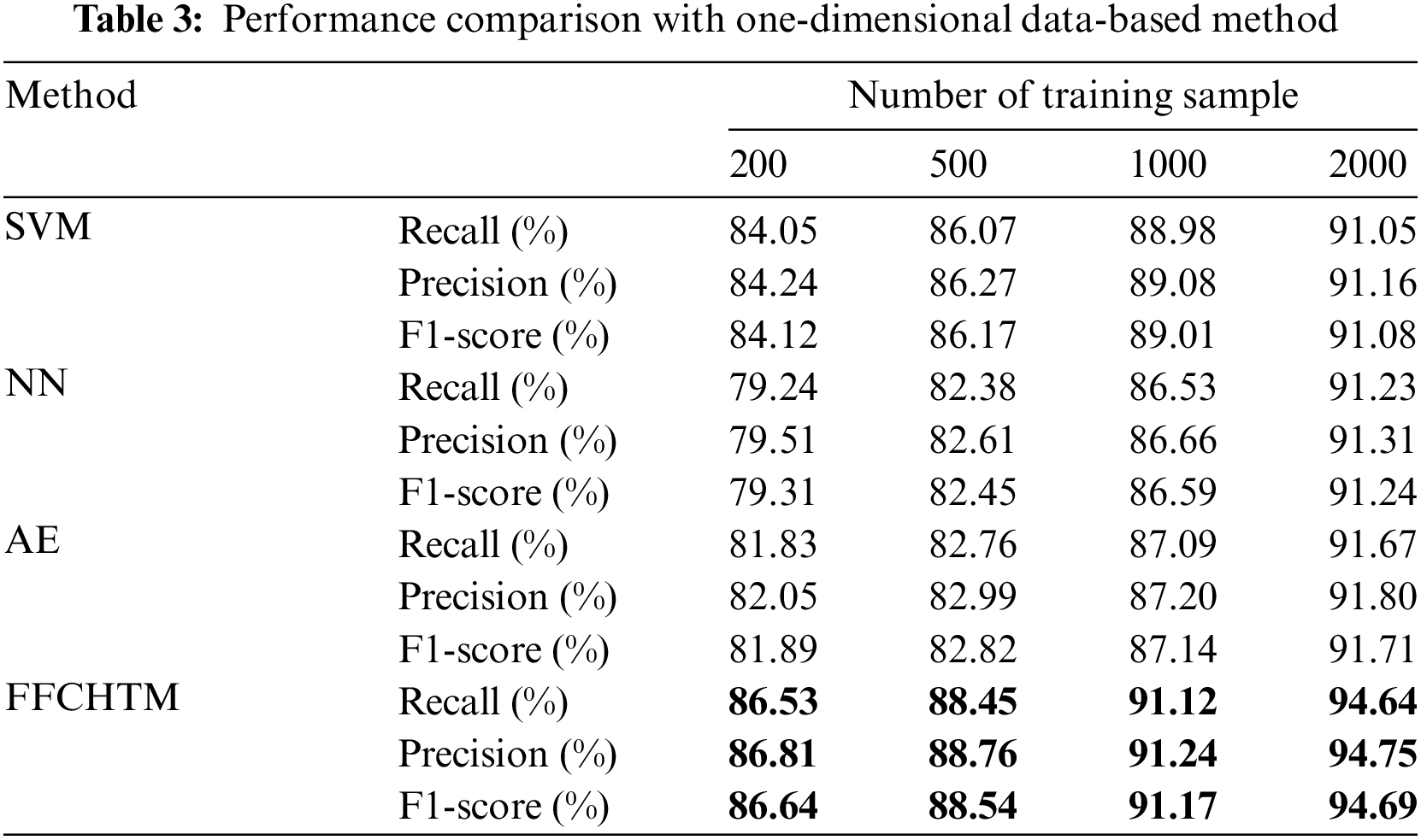
In general, having more data tends to result in improved performance in machine learning models. With an increase in the size of the training sample, there is an enhancement in the overall classification performance. In instances where the training dataset’s sample size is comparatively small, the FFCHTM and SVM models outperform the NN and AE models. This is because of the limited performance of NN and AE models, which is highly dependent on the number of samples. Moreover, FFCHTM models demonstrate better performance than SVM models across different training sample sizes. The reason for this is that image-form data can retain a greater amount of curve variations and trend details than data presented in a one-dimensional array format. Besides, the FFCHTM model takes tensor data as input, further facilitating spatial information learning.

4.3.3 Complexity Comparison

In this study, the SVM employing an RBF kernel, with a total training sample size of n and a feature count of five, exhibits a complexity of O(n2). In the case of a Neural Network comprising L layers, where each layer contains ui units (i = 1, 2, …, L), and the input feature count is d, the complexity for a single forward pass is estimated to be O(∑i=1L−1ui×ui+1). The computational complexity of an autoencoder is similar to that of a neural network, being contingent on the number of layers L, the number of units in each layer ui, and the number of training iterations. For FFCHTM, given a dataset comprising {χ+i∈RI1×I2×…×IN}i=1l+ and {χ−i∈RI1×I2×…×IN}i=1l−, where n=l++l−, represents the total number of training samples, and R signifies the rank in the CP decomposition, the computational complexity of FFCHTM is given as O(n2R2∑m=1NIm), with the sum ∑m=1NIm reflecting the combined dimensions of the feature tensor.

It is evident that NN and AE possess a higher computational complexity due to the extensive number of parameters present within their architectures. Conversely, FFCHTM and SVM boast lower computational complexities. Notably, FFSTM and SVM have computational complexities that fall within the same magnitude, explicitly O(n2).

4.4 Comparisons with the 2D Data-Based Method

4.4.1 Comparison Method

The developed fault diagnosis method is contrasted with the 2D data-based fault diagnosis approaches reported in the current literature. The comparative models include the Convolutional Autoencoder (CAE), CNN [19], and Standard Tensor Machine (STM) [35]. The model’s input is the stacked images with a size of 32 × 32 × 3, including train and test samples. The type of data is the three-phase current. The following are the specifics of the method and the necessary modifications to the parameters:

•   CAE. The encoder consists of a two-layer structure, each performing a 2D convolution and a 2D max-pooling operation. The initial and subsequent tiers comprise 16 and eight kernels, respectively, each measuring 3 × 3. The decoder utilizes a structure consisting of two layers, incorporating 2D deconvolution and 2D unpooling operations. Similar to the encoder, the initial and subsequent decoder layers are comprised of 16 and eight kernels, respectively, each having dimensions of 3 × 3. The pooling and unpooling kernel sizes are both set to 2 × 2. The model undergoes 20 iterations, starting with an initial learning rate of 0.001. The Adam optimizer is utilized for optimization, and the SoftMax function is employed as the activation function.

•   CNN.The structure of the model includes two layers, where the initial and subsequent layers comprise 16 and eight kernels, respectively, each having a dimension of 3 × 3. The 2 × 2 kernels are used by the pooling layers, which are connected to the first and second layers. The model undergoes 20 iterations, commencing with an initial learning rate of 0.001. It employs the Adam optimizer, and the SoftMax activation function is utilized for the optimization process.

•   STM. The type of data is the A-phase current. The search interval for the penalty factor C spans is [20, 210], whereas the kernel parameter σ’s search range is [2−2, 26].

4.4.2 Comparison Result

The evaluation trial for the 2D data-driven technique is performed using the dataset of three-phase current curves. The effectiveness of these schemes is assessed by employing n samples (with n being 200, 500, 1000, or 2000) for each data category. The test set comprises 300 randomly selected samples for each type. Table 4 illustrates the model’s performance metrics, specifically focusing on recall, precision, and F1-score.

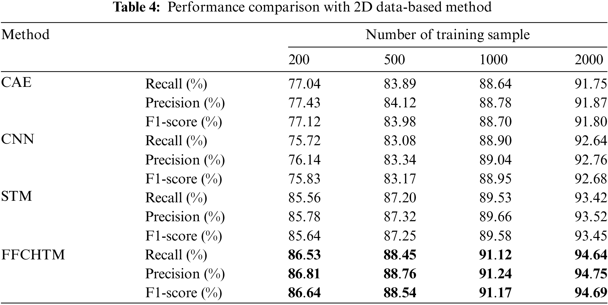
The superior performance of FFCHTM and STM compared to CAE and CNN is evident across various training sample quantities. The transition of the 2D feature map into a one-dimensional format via the flattening operation employed by CAE and CNN results in the loss of information related to spatial structure. Furthermore, although the STM model shows promising results, the multiple inner product operations of tensor features during the alternating projection solution process lead to a loss of spatial information, which impacts its performance. As a result, the scheme based on FFCHTM surpasses the STM-based approach in terms of overall performance.

4.4.3 Complexity Comparison

For CAE, considering the case that the number of convolutional layers in a neural network is D, the complexity is O(∑l=1DM2K2Cl−1Cl), where M2is the area of the feature map, K2 is the convolution kernel area, Cl denotes the number of output channels of the lthconvolutional layer. The computational complexity of CNN is similar to that of CAE. For the dataset {χ+i∈RI1×I2×…×IN}i=1l+ and {χ−i∈RI1×I2×…×IN}i=1l−, the computational complexity of STM is O((l++l−)2NT∑n=1NIn), T represents the number of iterations for the alternating projection method. FFCHTM’s computational complexity is O((l++l−)2R2∑n=1NIn).

It is clear that both CAE and CNN incur a higher computational complexity due to the large number of parameters intrinsic to their structures. On the other hand, FFCHTM and STM exhibit lower computational complexities. Notably, the computational complexity of FFCHTM is lower than STM’s because it employs a simpler optimization solution process.

4.5 Proposed Diagnosis Scheme Analysis

The effectiveness of the proposed scheme is confirmed by the outcomes of Experiment 1 and Experiment 2. By integrating spatial structure-related data and multi-mode monitoring data fusion, the proposed diagnostic scheme outperforms the existing methods. However, the occurrence of equipment failures in actual subway stations is extremely rare due to rigorous routine inspections, leading to a scarcity of fault data. This scarcity hampers the ability of the proposed approach to identify new fault categories. Moreover, as demonstrated in Experiment 1 and Experiment 2, the performance of the proposed approach is influenced by the size of the training datasets, revealing its limitations when dealing with small training sample sizes.

5  Conclusion

The present study suggests a fault diagnosis scheme for railway switch machine using FFCHTM. The scheme being presented involves three primary stages: 1) pre-processing of data, 2) generation of fusion feature tensor, and 3) implementation of tensor learning. The foremost contribution of this research lies in developing a data-driven fault diagnosis scheme for railway switch machines, which specifically considers the data’s unique characteristics and spatial information. The spatial structure-related data information is preserved and considered in data processing and modeling. Meanwhile, a data fusion-based tensor machine algorithm is designed to improve single signal data’s limitations in insufficient information. In the end, the established technique is assessed and confirmed using actual operational data.

This research requires adequate data for each category of samples to facilitate model training, and the construction process of feature tensors is time-consuming. Moreover, it is unable to recognize data associated with unknown fault types. Future research will focus on diagnosing turnout faults in scenarios with limited sample datasets. Novel methodologies for the construction of feature tensors will be investigated, ensuring both time efficiency and effectiveness. We will investigate a novel tensor learning model that can effectively utilize small samples to enhance the model’s performance in such scenarios. Furthermore, we will explore a framework that facilitates the automatic updating of the model to enable the diagnosis of new fault types.

Acknowledgement: The authors thank CASCO for contributing field knowledge and research data support.

Funding Statement: This research work is supported by the National Key Research and Development Program of China under Grant 2022YFB4300504-4 and the HKRGC Research Impact Fund under Grant R5020-18.

Author Contributions: The authors confirm the following contributions: Study conception and design: Chen Chen; data collection: Zhongwei Xu, Meng Mei; analysis and interpretation of results: Chen Chen, Kai Huang; draft manuscript preparation: Chen Chen, Meng Mei, Siu Ming Lo. The results were reviewed and approved by all authors.

Availability of Data and Materials: Not applicable.

Conflicts of Interest: The authors affirm that there are no conflicts of interest associated with this research.

References

1. Z. Zhu, “China’s urban rail transit trips skyrocket 130% in December 2023. China Daily,” 2024. Accessed: Jan. 13, 2024, [Online]. Available: https://www.chinadaily.com.cn/a/202401/13/WS65a2590 [Google Scholar]

2. C. Chen, X. Q. Li, K. Huang, Z. W. Xu, and M. Mei, “A convolutional autoencoder based fault detection method for metro railway turnout,” Comput. Model. Eng. Sci., vol. 136, no. 1, pp. 471–485, 2023. doi: 10.32604/cmes.2023.024033 [Google Scholar] [CrossRef]

3. M. Hamadache, S. Dutta, O. Olaby, R. Ambur, E. Stewart and R. Dixon, “On the fault detection and diagnosis of railway switch and crossing systems: An overview,” Appl. Sci., vol. 9, no. 23, pp. 5129, 2019. doi: 10.3390/app9235129. [Google Scholar] [CrossRef]

4. J. Lin, H. Shao, X. Zhou, B. Cai, and B. Liu, “Generalized MAML for few-shot cross-domain fault diagnosis of bearing driven by heterogeneous signals,” Expert. Syst. Appl., vol. 230, no. 3, pp. 120696, 2023. doi: 10.1016/j.eswa.2023.120696. [Google Scholar] [CrossRef]

5. S. Yan, X. Zhong, H. Shao, Y. Ming, C. Liu and B. Liu, “Digital twin-assisted imbalanced fault diagnosis framework using subdomain adaptive mechanism and margin-aware regularization,” Reliab. Eng. Syst. Saf., vol. 239, no. 1, pp. 109522, 2023. doi: 10.1016/j.ress.2023.109522. [Google Scholar] [CrossRef]

6. J. Yin, T. Tang, L. Yang, J. Xun, Y. Huang and Z. Gao, “Research and development of automatic train operation for railway transportation systems: A survey,” Transp. Res. Part C: Emerg. Technol., vol. 85, no. 3, pp. 548–572, 2017. doi: 10.1016/j.trc.2017.09.009. [Google Scholar] [CrossRef]

7. H. Shao, W. Li, B. Cai, J. Wan, Y. Xia and S. Yan, “Dual-threshold attention-guided GAN and limited infrared thermal images for rotating machinery fault diagnosis under speed fluctuation,” IEEE Trans. Ind. Inform., vol. 19, no. 9, pp. 9933–9942, 2023. doi: 10.1109/TII.2022.3232766. [Google Scholar] [CrossRef]

8. S. Yan, H. Shao, Z. Min, J. Peng, B. Cai and B. Liu, “FGDAE: A new machinery anomaly detection method towards complex operating conditions,” Reliab. Eng. Syst. Saf., vol. 236, no. 2, pp. 109319, 2023. doi: 10.1016/j.ress.2023.109319. [Google Scholar] [CrossRef]

9. H. Pan, H. Xu, J. Zheng, H. Shao, and J. Tong, “A semi-supervised matrixized graph embedding machine for roller bearing fault diagnosis under few-labeled samples,” IEEE Trans. Ind. Inform., vol. 20, no. 1, pp. 1–9, 2024. doi: 10.1109/TII.2023.3265525. [Google Scholar] [CrossRef]

10. W. Li and G. Li, “Railway’s turnout fault diagnosis based on power curve similarity,” in Int. Conf. Commun., Inf. Syst. Comput. Eng. (CISCE), Haikou, China, 2019, pp. 112–115. [Google Scholar]

11. H. Kim, J. Sa, Y. Chung, D. Park, and S. Yoon, “Fault diagnosis of railway point machines using dynamic time warping,” Electron. Lett., vol. 52, no. 10, pp. 818–819, 2016. doi: 10.1049/el.2016.0206. [Google Scholar] [CrossRef]

12. S. Huang, X. Yang, L. Wang, W. Chen, F. Zhang and D. Dong, “Two-stage turnout fault diagnosis based on similarity function and fuzzy c-means,” Adv. Mech. Eng., vol. 10, no. 12, 2018. doi: 10.1177/1687814018811402. [Google Scholar] [CrossRef]

13. F. C. O. F. Eker and U. Kumar, “SVM based diagnostics on railway turnouts,” Int. J. Perform. Eng., vol. 8, no. 3, pp. 289–398, 2012. [Google Scholar]

14. C. An, F. Gan, W. Luo, and F. Qin, “Method of speed-up turnout fault diagnosis using wavelet packet energy entropy,” J. Railw. Sci. Eng., vol. 12, no. 2, pp. 269–274, 2015. [Google Scholar]

15. Z. Wang et al., “Segmentalized mRMR features and cost-sensitive ELM with fixed inputs for fault diagnosis of high-speed railway turnouts,” IEEE Trans. Intell. Transp. Syst., vol. 24, no. 5, pp. 4975–4987, 2023. doi: 10.1109/TITS.2023.3239636. [Google Scholar] [CrossRef]

16. Y. Sun, Y. Cao, P. Li, and S. Su, “Sound based degradation status recognition for railway point machines based on soft-threshold wavelet denoising, WPD and ReliefF,” IEEE Trans. Instrum. Meas., vol. 73, no. 1, pp. 1–9, 2024. doi: 10.1109/TIM.2023.3334370. [Google Scholar] [CrossRef]

17. Y. Cao, Y. Sun, P. Li, and S. Su, “Vibration-based fault diagnosis for railway point machines using multi-domain features, ensemble feature selection and SVM,” IEEE Trans. Vehicular Technol., vol. 73, no. 1, pp. 176–184, 2024. doi: 10.1109/TVT.2023.3305603. [Google Scholar] [CrossRef]

18. Y. Xiao, H. Shao, M. Feng, T. Han, J. Wan and B. Liu, “Towards trustworthy rotating machinery fault diagnosis via attention uncertainty in transformer,” J. Manuf. Syst., vol. 70, no. 9, pp. 186–201, 2023. doi: 10.1016/j.jmsy.2023.07.012. [Google Scholar] [CrossRef]

19. P. Zhang, G. Zhang, W. Dong, X. Sun, and X. Ji, “Fault diagnosis of high-speed railway turnout based on convolutional neural network,” in Int. Conf. Autom. Comput. (ICAC), Newcastle, UK, 2018, pp. 1–6. [Google Scholar]

20. M. Li and R. Fei, “Research and implementation of fault diagnosis of switch machine based on data enhancement and CNN,” in IEEE Int. Conf. Trust, Secur. Privacy in Comput. Commun. (TrustCom), Wuhan, China, 2022, pp. 1467–1472. [Google Scholar]

21. Z. Lao, D. He, Z. Jin, C. Liu, H. Shang and Y. He, “Few-shot fault diagnosis of turnout switch machine based on semi-supervised weighted prototypical network,” Knowl. Based Syst., vol. 274, no. 1, pp. 110634, 2023. doi: 10.1016/j.knosys.2023.110634. [Google Scholar] [CrossRef]

22. M. Li, X. Hei, W. Ji, L. Zhu, Y. Wang and Y. Qiu, “A fault-diagnosis method for railway turnout systems based on improved autoencoder and data augmentation,” Sensors, vol. 22, no. 23, pp. 9438, 2022. doi: 10.3390/s22239438. [Google Scholar] [PubMed] [CrossRef]

23. Z. Guo, Y. Wan, and H. Ye, “An unsupervised fault-detection method for railway turnouts,” IEEE Trans. Instrum. Meas., vol. 69, no. 11, pp. 8881–8901, 2020. doi: 10.1109/TIM.2020.2998863. [Google Scholar] [CrossRef]

24. Y. Ye, C. Huang, J. Zeng, Y. Zhou, and F. Li, “Shock detection of rotating machinery based on activated time-domain images and deep learning: An application to railway wheel flat detection,” Mech. Syst. Signal. Process., vol. 186, no. 10, pp. 109856, 2023. doi: 10.1016/j.ymssp.2022.109856. [Google Scholar] [CrossRef]

25. Y. Ye, B. Zhu, P. Huang, and B. Peng, “OORNet: A deep learning model for on-board condition monitoring and fault diagnosis of out-of-round wheels of high-speed trains,” Measurement, vol. 199, no. 2, pp. 111268, 2022. doi: 10.1016/j.measurement.2022.111268. [Google Scholar] [CrossRef]

26. Z. He, H. Shao, J. Cheng, Y. Yang, and J. Xiang, “Kernel flexible and displaceable convex hull based tensor machine for gearbox fault intelligent diagnosis with multi-source signals,” Measurement, vol. 163, pp. 107965, 2020. doi: 10.1016/j.measurement.2020.107965. [Google Scholar] [CrossRef]

27. Z. He, J. Cheng, J. Li, and Y. Yang, “Linear maximum margin tensor classification based on flexible convex hulls for fault diagnosis of rolling bearings,” Knowl. Based Syst., vol. 173, no. 2, pp. 62–73, 2019. doi: 10.1016/j.knosys.2019.02.024. [Google Scholar] [CrossRef]

28. M. Zeng, Y. Yang, J. Zheng, and J. Cheng, “Maximum margin classification based on flexible convex hulls for fault diagnosis of roller bearings,” Mech. Syst. Signal. Process., vol. 66-67, no. 6, pp. 533–545, 2016. doi: 10.1016/j.ymssp.2015.06.006. [Google Scholar] [CrossRef]

29. M. Zeng, Y. Yang, S. Luo, and J. Cheng, “One-class classification based on the convex hull for bearing fault detection,” Mech. Syst. Signal. Process., vol. 81, no. 4, pp. 274–293, 2016. doi: 10.1016/j.ymssp.2016.04.001. [Google Scholar] [CrossRef]

30. C. Cortes and V. Vapnik, “Support-vector networks,” Mach. Learn., vol. 20, no. 3, pp. 273–297, 1995. doi: 10.1007/BF00994018. [Google Scholar] [CrossRef]

31. Y. Zhang, X. Deng, and Y. Huang, “Research on railroad turnout fault diagnosis based on support vector machine,” in Int. Sym. Mechatron. Indust. Inform. (ISMII), Zhuhai, China, 2021, pp. 119–122. [Google Scholar]

32. K. Zhang, “The railway turnout fault diagnosis algorithm based on BP neural network,” in IEEE Int. Conf. Control Sci. Syst. Eng., Yantai, China, 2014, pp. 135–138. [Google Scholar]

33. Z. Guo, H. Ye, W. Dong, X. Yan, and Y. Ji, “A fault detection method for railway point machine operations based on stacked autoencoders,” in Int. Conf. Autom. Comput. (ICAC), Newcastle, UK, 2018, pp. 1–6. [Google Scholar]

34. B. Nayana and P. Geethanjali, “Analysis of statistical time-domain features effectiveness in identification of bearing faults from vibration signal,” IEEE Sens. J., vol. 17, no. 17, pp. 5618–5625, 2017. doi: 10.1109/JSEN.2017.2727638. [Google Scholar] [CrossRef]

35. D. Tao, X. Li, W. Hu, S. Maybank, and X. Wu, “Supervised tensor learning,” in IEEE Int. Conf. Data Mining (ICDM’05), Houston, USA, 2005, pp. 8–16. [Google Scholar]