A Combination Prediction Model for Short Term Travel Demand of Urban Taxi

1  Introduction

The rapid development of the internet and transportation has led to a notable diversification in passengers’ travel modes [1]. However, the indiscriminate search for passengers by unoccupied taxi drivers has resulted in a pronounced temporal and spatial imbalance in taxi supply and demand, further exacerbating urban traffic congestion issues. Therefore, effective prediction of taxi travel demand within a specific region is important for achieving effective urban taxi dispatching and preventing urban traffic congestion [2,3].

Taxi travel demand is affected by external factors such as weather and holidays, and is characterized by non-linearity, non-smoothness and spatio-temporal correlation [4]. At present, considerable research efforts by experts and scholars have been dedicated to short-term traffic flow prediction, encompassing both linear and non-linear models. Traditional linear prediction models, such as time series prediction models [5] and Kalman filter models [6], have found widespread application in predicting passenger flow. Despite their widespread adoption, these models often exhibit low computational efficiency and significant prediction errors, particularly when confronted with the intricate and highly nonlinear nature of current short-term traffic flow scenarios [7]. Nonlinear prediction models, including grey theory [8], support vector machine [9], and neural network model [10], offer effective solutions to the aforementioned challenges. For example, Yuan et al. [11], employing a two-dimensional approach involving time and space, formulated a passenger flow prediction method based on a Bayesian network. However, due to the increasing scale and complexity of taxi flow data, this type of model is no longer able to capture the features in taxi flow data well, resulting in a decrease in prediction efficiency [12].

In recent years, the rapid advancements in data mining, machine learning, and related technologies have given rise to numerous deep learning methods, demonstrating an aptitude for capturing intricate nonlinear relationships and associated features within traffic flow data [13]. These models have significantly enhanced the precision of passenger flow prediction, gaining widespread application in traffic flow forecasting. Zhu et al. [14] combined deep learning theory with support vector machines to construct a Support Vector Machine Based on Deep Learning (DL-SVM) model for passenger flow prediction in urban rail transit, due to the significant temporal and spatial correlation of traffic flow between road sections. Han et al. [15] transformed the subway network into a graph and established a graph convolutional neural network (GCNN) for passenger flow prediction, demonstrating good performance and interpretability. Liu et al. [16] introduced an Attention-based Multiple Graph Convolutional Recurrent Network to capture dynamic and potential spatiotemporal correlations in traffic flow data. Recurrent Neural Network (RNN) and Convolutional Neural Network (CNN) are mainstream deep learning models. RNN is particularly powerful in modeling temporal data, and CNN can more effectively capture the spatial correlation of data, but both are relatively prone to the problem of gradient vanishing. To solve this problem, Long Short-Term Memory Neural Networks (LSTM) have emerged, which rely on gating mechanisms to solve gradient vanishing and exploding problems, and are suitable for longer time series. They are widely used by many scholars in traffic flow prediction [16–19]. For example, Du et al. [20] introduced a method for urban traffic passenger flow prediction based on LSTM, demonstrating superior results compared to traditional prediction models. Shi et al. [21] took an innovative approach by first extracting features from passenger flow data through principal component analysis (PCA) and subsequently constructing a prediction model based on LSTM. Lu et al. [22] proposed a short-term traffic flow prediction method based on Autoregressive Integrated Moving Average Model (ARIMA) and LSTM neural networks. Zhang et al. [23] considered weather and holiday events and used a residual neural network framework to model the temporal compactness, periodicity, and trend characteristics of crowd traffic.

The above findings demonstrate the remarkable performance of deep neural networks in predicting traffic flow using big data. Despite these advancements, our comprehension of traffic flow data remains constrained, and there persists an ongoing challenge in fully harnessing the intricate features of traffic flow to enhance performance while accommodating external influences. First, the analysis of traffic flow data confronts obstacles arising from factors like incomplete or inaccurate data collection, exerting an impact on the accuracy and reliability of predictions. Second, despite the inclusion of external influences in the modeling process, there exists a challenge in fully capturing and integrating these factors into the prediction model, thereby constraining its overall effectiveness.

The evolution of computer network signals has revealed striking similarities between signals and traffic flow. Researchers have leveraged this insight, introducing signal decomposition algorithms to process traffic flow data, consequently leading to substantial improvements in prediction accuracy [24]. Li et al. [25] proposed a prediction framework based on empirical mode decomposition and support vector regression (EMD-SVR). Compared with the traditional passenger flow prediction methods, the prediction accuracy has been significantly improved. Cao et al. [26] verified that the Ensemble Empirical Mode Decomposition (EEMD) is more suitable for traffic prediction than the Empirical Mode Decomposition (EMD). However, the noise residue problem and computational complexity of the EEMD algorithm are relatively high.

Due to the characteristics of taxi travel demand, traditional time-series models struggle to effectively learn deep features in the data [27,28]. To improve the prediction accuracy, this paper proposes a combined prediction model combining CEEMDAN [29] and ConvLSTM [30], Among them, CEEMDAN analyzes and processes the taxi travel demand data to reduce the data complexity, and ConvLSTM learns the spatio-temporal correlation based on the processed taxi travel demand data. The main contributions of this study are as follows:

(1) CEEMDAN Decomposition. The CEEMDAN method is suitable for dealing with nonlinear and complex taxi travel demand data, and is able to capture the characteristics of different time scales and frequencies in the data, which in turn reduces the complexity of taxi travel demand data and improves the predictability of the data.

(2) Sample Entropy Evaluation. The modal components after decomposition still have the problem of modal aliasing, therefore, the sample entropy is used to assess the complexity of the components and the components are reconstructed using the K-means clustering algorithm, which avoids the waste of arithmetic power and at the same time reduces the cumulative prediction error of each component sequence.

(3) ConvLSTM Neural Network Model. Considering the spatiotemporal correlation between external factors such as weather conditions, holidays, and taxi traffic, a ConvLSTM neural network model is constructed. This model incorporates the LSTM time series processing capability and CNN spatial feature processing ability, the model can effectively explore the spatio-temporal correlation in the cab travel demand data, and then obtain more accurate prediction results.

Section 2 delineates the framework of the combined CEEMDAN-ConvLSTM prediction model, elucidating the innovative approach proposed in this study. Section 3 delves into the decomposition and reconstruction modules within the framework. Section 4 expounds upon the prediction module encapsulated within the proposed framework. Section 5 engages in a comprehensive case study, comparing and analyzing the efficacy of our proposed model against mainstream benchmark models in the field. The objective is to assess and validate the effectiveness of our prediction model. Lastly, Section 6 encapsulates the culmination of this work, presenting a summary of the findings and offering insights for future directions in this domain.

2  Proposed Methodology

This study proposes a taxi travel demand prediction model based on CEEMDAN ConvLSTM, and the overall framework of the model is shown in Fig. 1. This mainly includes two parts: (1) Decomposition and reconstruction module of temporal data, which performs modal decomposition and reconstruction on taxi travel demand data. (2) The taxi travel demand prediction module predicts and fuses the reconstructed components to generate the final prediction result. The proposed methodology, through the integration of decomposition, reconstruction, and prediction, endeavors to provide a robust and accurate prediction model for taxi travel demand. The subsequent sections delve into each module in detail, elucidating the intricacies of their respective processes.

Figure 1: Overall prediction framework

3  Decomposition and Reconstruction of Taxi Travel Demand

3.1 CEEMDAN Algorithm

The CEEMDAN algorithm mitigates the problem of modal aliasing in the EMD algorithm by introducing adaptive Gaussian white noise at each stage of decomposition. This model diminishes the noise residue of the EEMD algorithm, and enhances the completeness of the decomposition process, resulting in an almost zero reconstruction error. The decomposition process of the algorithm is illustrated in Fig. 2, and the details are as follows:

Figure 2: The CEEMDAN decomposition algorithm

(1) Add Gaussian white noise ε0ωi(t) with initial amplitude ε0 to the original signal yt, (i = 1, 2,..., I), where ωi(t) is a white noise sequence that follows a standard normal distribution, to obtain a new signal yi(t)=y(t)+ε0ωi(t). The new signal is decomposed by EMD to obtain the i modal components of the first stage IMF1i. The overall average of modal components can be obtained from the first eigenmodal components of CEEMDAN decomposition IMF1:

IMF1=1I∑i=1IIMF1i(1)

(2) Calculate the residual error after removing the first modal component:

r1(t)=yi(t)−IMF1(2)

(3) Define Ek represent the Kth modal component obtained by EMD decomposition. Add the noise component ε1E1(ωi(t)) to the residual r1(t), and then decompose to get the second-order modal component as follows:

IMF2=1I∑i=1IE1(r1(t)+ε1E1(ωi(t)))(3)

(4) Repeat steps (2), (3), for k = 1,2,..., n, to get the residual after removing the Kth component and the K+1th modal component:

rk(t)=rk−1(t)−IMFk(4)

IMFk+1=1I∑i=1IE1(rk(t)+εkEk(ωi(t)))(5)

(5) When the residual rk(t) cannot continue to decompose, the decomposition terminates. The final residual signal is:

rn(t)=yi(t)−∑k=1nIMFk(6)

3.2 Component Evaluation and Reconstruction

After the completion of the modal decomposition, using the IMF component directly as the prediction model input results in a substantial computational load, potentially leading to error accumulation. To address this, sample entropy [31] is employed for assessing component complexity and as a reference for subsequent component reconstruction, as illustrated in Fig. 3.

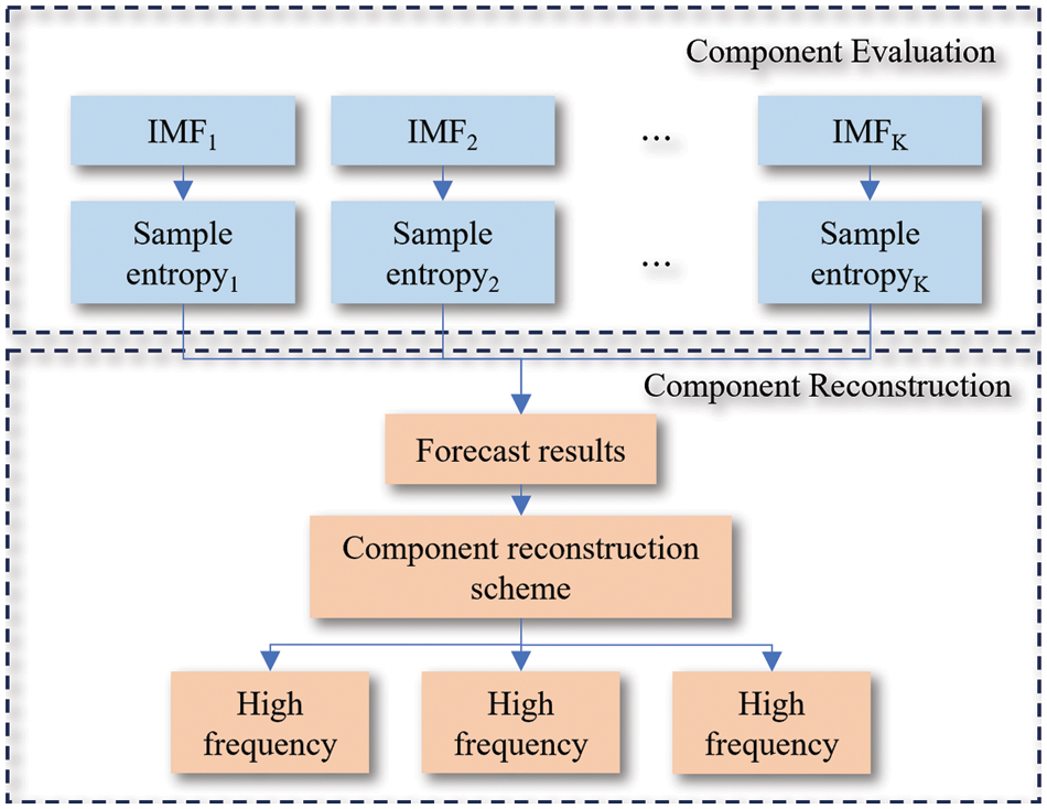
Figure 3: Component evaluation and reconstruction

Sample entropy, as a model-free method, presents several advantages in evaluating data complexity. Firstly, it requires no prior knowledge or assumptions, making it directly applicable to various data types, thereby enhancing flexibility and analysis applicability. Secondly, sample entropy can measure the diversity and uncertainty of data. A higher sample entropy indicates more complex data, greater variability, and diversity, offering significant value in studying and analyzing intricate datasets. Furthermore, sample entropy is not constrained by data dimensions or distributions, making it suitable for high-dimensional and nonlinear data. It proves useful in the analysis of multimodal data and plays a pivotal role in comparing and evaluating decomposition results. In summary, as a model-free method, sample entropy demonstrates broad applicability and strong adaptability across diverse data types and high-dimensional datasets. Its notable advantages lie in its wide-ranging application, making it a crucial indicator for evaluating component complexity.

The K-means clustering algorithm has advantages, including simplicity, scalability, interpretability, robustness, and parallelism. These advantages make the K-means algorithm a widely utilized and effective clustering method, well-suited for processing large-scale high-dimensional datasets, and able to interpret and visualize clustering results. At the same time, it also has a certain degree of fault tolerance and parallelism processing ability. Therefore, this algorithm is employed for clustering the evaluated results.

4  The Prediction Model for Taxi Travel Demand

To achieve effective short-term taxi travel demand prediction across diverse city areas, it is imperative to consider series encompassing spatial and temporal structures. The LSTM network proves to be well-suited for processing time series data. As a variant of recurrent neural networks, it addresses the gradient disappearance issue by introducing a “gate control” mechanism, enhancing the neural network’s memory capacity compared to the traditional RNN model. In the LSTM architecture, input data at each time step undergoes processing through the structures of the “forget gate,” “input gate,” “candidate gate,” and “output gate.” These gate control mechanisms regulate information flow within the network by dynamically adjusting their respective weights in real-time. This approach a empowers LSTM to effectively capture long-term dependencies, fulfilling the requirements for sustained memory in network data. The formulas governing the “forget gate,” “input gate,” “candidate gate,” and “output gate” in the LSTM network are presented as follows:

it=σ(Wxixt+Whiht−1+Wci∘ct−1+bi)ft=σ(Wxfxt+Whfht−1+Wcf∘ct−1+bf)ct=ft∘ct−1+it∘tanh⁡(Wxcxt+Wxcht−1+bc)ot=σ(Wxoxt+Whoht−1+Wco∘ct+bo)ht=ot∘tanh⁡(ct)(7)

where, σ is the sigmoid or tanh function, Wxi,Wxf,Wxc,Wxo respectively are the node weight matrix of “input gate”, “forget gate”, “memory unit” and “output gate” bi, bf, bc, bo respectively are the node threshold matrix of “input gate”, “forget gate”, “memory unit” and “output gate”. However, the model makes it difficult to extract local spatial features. To solve this problem, the ConvLSTM network is used to replace the dot product operation in the original LSTM with the convolution operation. The core idea behind ConvLSTM is to introduce convolution operations into the cyclic structure of LSTM to capture the local features and global association information of spatiotemporal sequences. This enhancement enables the ConvLSTM network to effectively deal with prediction problems associated with spatiotemporal series. The structure of the model is shown in Fig. 4.

Figure 4: The ConvLSTM network structure

Where, it control the “input gate”, which controls the selection of new data and the output of the previous neuron. The input gate determines what information the neuron receives. ft control “forget gate”, forgetting the output of the previous neuron in proportion to controlling how much information from the previous neuron is retained to enter that neuron. ct is the cell state of the time t neuron, which combines the cell state of the previous neuron with the input of time t to form a new cell state. The “output gate” outputs the cell state in proportion to the current cell state as the output of this cell through the gating mechanism. The following is the calculation formula for each variable in the ConvLSTM network:

it=sigmoid(Wxi∗Xt+Whi∗ht−1+Wci∘ct−1+bi)ft=sigmoid(Wxf∗Xt+Whf∗ht−1+Wcf∘ct−1+bf)ct=ft∘ct−1+it∘tanh⁡(Wxc∗Xt+Wxc∗ht−1+bc)ot=sigmoid(Wxo∗Xt+Who∗ht−1+Wco∘ct+bo)ht=ot∘tanh⁡(ct)(8)

where, Wxi, Wxf, Wxc, Wxo respectively are the weights in different convolution operations, and bi, bf, bc, bo respectively are the biases of convolution operations. “*” denotes the convolution operation. Xt is the input of the neuron at time t; ht−1 is the output of the neuron at time t-1.

5  Experimental Process and Analysis

5.1 Dataset and Experimental Environment

The experiments detailed in this article were carried out on servers with the following device specifications: CPU-Intel (R) Core (TM) i7-12600K, GPU-NVIDIA GeForce RTX 4070, and operating system-Windows 11. The algorithms and models were implemented using the Python language.

The data used in the experimental part of this study includes two parts: (1) Taxi travel demand data for a certain area in Beijing from November 2015 to April 2016. Obtain the demand for taxi boarding and alighting in the region through statistical analysis of taxi boarding and alighting points; (2) The weather data of Beijing from November 2015 to April 2016 and the statutory holidays in China. Refer to Fig. 5 for a comprehensive overview of the various datasets employed in this study.

Figure 5: The various temporal data used in this study

Fig. 5 facilitates a more intuitive comprehension of taxi traffic data characteristics. Primarily, it is evident that taxi traffic data displays a non-linear trend, showcasing curve-like fluctuations rather than adhering to a linear trajectory. Secondly, the data demonstrates nonstationary, revealing trends and fluctuations over time rather than maintaining a constant pattern. Additionally, taxi traffic data exhibits periodicity, indicating a discernible pattern or regularity within a specified time range. In the holiday data, numerical values are assigned as follows: 0 denotes working days and compensatory days, 1 denotes weekends, and 2 denotes statutory holidays, such as the Spring Festival.

5.2 Taxi Time Series Data Decomposition

5.2.1 Data Decomposition

Applying the CEEMDAN decomposition algorithm as detailed in Section 2.1.1, the taxi travel demand data associated with boarding and alighting in the specified region undergoes decomposition into multi-component Intrinsic Mode Functions (IMF) and residual components of different orders. The results of this decomposition are visually presented in Fig. 6.

Figure 6: Decomposition results of taxi boarding and alighting demand

Upon observing diverse modalities within taxi travel demand data, insights into the characteristics and fluctuations in taxi demand based on the frequency and complexity of these modalities can be gleaned. Primarily, through the decomposition results, the complexity of the data can be discerned by considering the frequency arrangement of the components. High-frequency components signify rapid changes and complexity in taxi demand, potentially linked to short-term events or specific situations. For instance, peak hours during the day or particular holidays may lead to abrupt increases or decreases in demand.

Low-frequency components signify relatively stable trends and alterations. These components may be associated with long-term trends or major influencing factors, such as economic development levels and market competition. Monitoring changes in low-frequency components enables comprehension of the overarching trends and influencing factors in taxi demand.

Furthermore, analyzing residual components aids in understanding special situations or aspects of taxi demand data not elucidated by the main components. Residual components may encompass random noise or other data that remains unaccounted for by the primary components.

5.2.2 Component Reconstruction

For multiple IMF components obtained through modal decomposition, direct prediction can incur a significant computational burden and easily lead to error accumulation. Therefore, it is necessary to reconstruct the decomposed components through appropriate standards and methods. According to the evaluation method in Section 3.2, the sample entropy index is used to evaluate the components and the evaluation results are shown in Fig. 7.

Figure 7: Component evaluation index values

According to the calculation results of sample entropy, the sample entropy of each component decomposed by the algorithm gradually decreases with the decrease in frequency. This trend implies that, as the decomposition process progresses, the complexity of the obtained IMF components gradually decreases. Based on the evaluation results of sample entropy, the K-means clustering algorithm is used for clustering to obtain a component reconstruction scheme, as shown in Fig. 8.

Figure 8: Component reconstruction scheme

According to the component reconstruction scheme in Fig. 8, the decomposed components depicted in Fig. 6 undergo reconstruction. The final reconstructed components are categorized into “High-frequency component,” “Medium-frequency component,” and “Low-frequency component.” The visualization of the reconstruction results is presented in Fig. 9.

Figure 9: Component reconstruction results of taxi boarding and alighting demand

Throughout the reconstruction process, we first merge components with similar frequencies, including low frequency, frequency, and mediate frequency components, as well as residual components. This amalgamation of components with analogous frequencies aims to diminish redundant information within the data and extract more representative features. Specifically, for the “Low-frequency component”, a summation operation is executed on lower-frequency components to yield smoother and more comprehensive low-frequency components. These components typically encapsulate long-term trends and gradual shifts in the data. Similarly, for the “High-frequency component,” analogous frequency high-frequency components undergo summation to generate smoother and more holistic high-frequency components. This process aids in amalgamating subtle vibrations and swift changes within high-frequency components, thereby mitigating noise in the data. Furthermore, the merging of the “Medium frequency component” and the residual component is imperative. The “Medium frequency component” typically embodies moderate changes and fluctuations in the data, while the residual component comprises randomness or noise unexplained by other frequency ranges. Integrating these components enhances our ability to capture mesoscale changes and irregularities within the data. The overarching objective of component reconstruction is to alleviate excessive decomposition and modal aliasing issues inherent in decomposition algorithms. This process concurrently reduces randomness and nonlinearity in the reconstructed data, thereby enhancing the predictability of temporal data. Additionally, component reconstruction contributes to a reduction in computational complexity, fostering more efficient and accurate analyses and applications.

5.3 Model Training and Testing

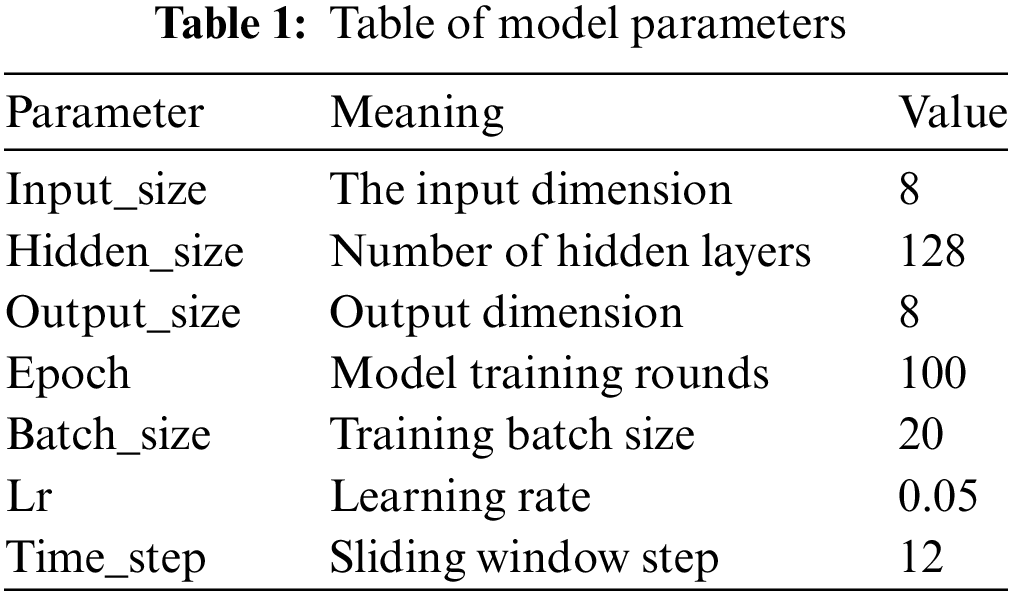
External factors, such as weather, and the decomposed components are individually input into their respective ConvLSTM models for training. The training parameters for the ConvLSTM model are pre-defined before commencing the training process, as detailed in Table 1.

Each reconstructed component is divided into training, validation, and testing sets in chronological order, with the following divisions: 70%, 10%, and 20%, respectively. The three ConvLSTM models use the training set and validation set in the training process. The loss rate variation curves of the “High-frequency component”, “Medium frequency component”, and “Low-frequency component” during the training process are shown in Fig. 10.

Figure 10: Changes in loss rate during the training process of three components

The graphical representation reveals distinct features among components during the training process. The “High-frequency component” experiences pronounced oscillations, indicating higher complexity and a greater fitting challenge, leading to substantial fluctuations in the model loss. In contrast, the training losses for the “Low-frequency component” and “Medium frequency component” exhibit comparatively stable patterns. The overall trend of the model’s loss curves during the training phase on both the training and validation sets displays a gradual descent, indicating the model’s convergence. This convergence is achieved relatively swiftly. As the loss on the training set diminishes, the loss on the validation set follows suit, gradually decreasing and stabilizing. This observation suggests that the model does not exhibit overfitting across diverse datasets, yielding more favorable training outcomes.

The trained model is used to test the CEEMDAN-ConvLSTM model in this study using a component test set of taxi alighting demand and boarding demand. The predicted results of the model are shown in Fig. 11.

Figure 11: The prediction of taxi boarding and alighting demand

Based on the results depicted in the figure, it is evident that the CEEMDAN ConvLSTM model performs well in predicting the travel demand for taxis in the region. The model demonstrates a commendable ability to accurately capture the evolving trends in taxi travel demand, showcasing its potential in tasks related to temporal data prediction. However, concerning the “High-frequency component”, we also noticed some challenges. Due to the high complexity of the “High-frequency component”, the model may encounter certain difficulties in predicting the “High-frequency component”, resulting in poor prediction accuracy. This issue may be caused by rapid changes in high-frequency components and subtle vibrations.

To further evaluate the accuracy of the prediction results, a quantitative analysis is imperative. This includes comparing with actual observation data, as well as using appropriate evaluation indicators to measure the accuracy and bias of prediction results. Through this comparison with observed data, the model’s efficacy in predicting taxi travel demand can be thoroughly evaluated, providing insights into its accuracy and reliability.

5.4 Comparative Analysis of Experimental Results

The evaluation indexes used in this paper include SMAPE (Symmetric Mean Absolute Percentage Error), RMSE (Root Mean Square Error), MAE (Mean Absolute Error), and R2 (Coefficient of Determination). The values of each evaluation index obtained using the CEEMDAN-ConvLSTM model are shown in Table 2.

To further validate the effectiveness of the prediction model constructed in this article, the same dataset was used to train and test LSTM, ARIMA, CNN, ConvLSTM, EEMD ConvLSTM, and non reconstructed CEEDMAN ConvLSTM models. The predictive effect of each model on the taxi boarding demand in the test set is presented in Fig. 12.

Figure 12: Prediction results of taxi boarding demand for each model

The comparative analysis presented in Fig. 12 highlights the predictive efficacy of the proposed model to other benchmark models. Generally, all models, except for CNN, demonstrate a commendable ability to accurately forecast the trends in taxi travel demand. A detailed examination reveals that, in comparison to other models, the model introduced in this study aligns more closely with actual data, exhibiting particularly precise predictions during peak periods of taxi travel demand.

The prediction results of the various models are quantitatively analyzed through the various indicators proposed above, and the comparison results are shown in Table 3.

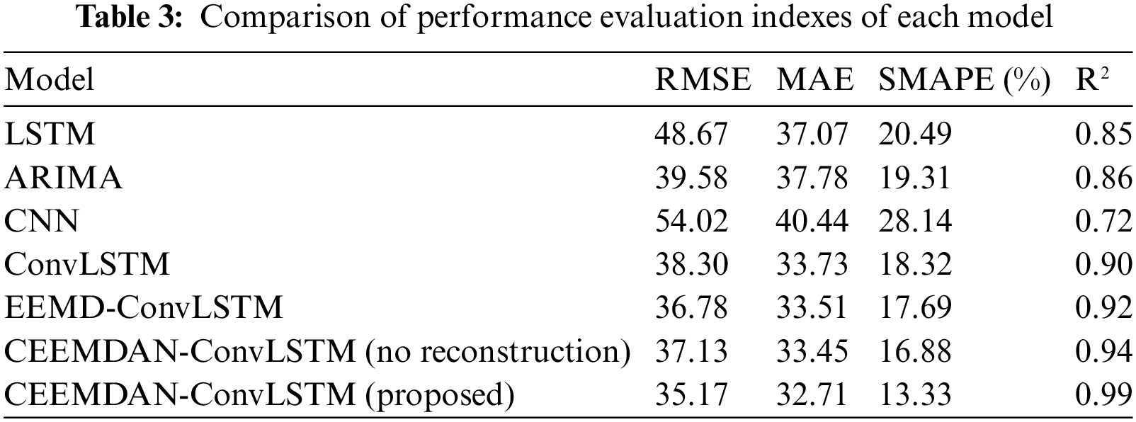
Comparing the evaluation metrics of commonly used LSTM, ARIMA, CNN, and ConvLSTM models, it is evident that the predictive performance of the model proposed in this paper is significantly enhanced with the integration of the time series decomposition algorithm. It is demonstrated that the ConvLSTM model can effectively deal with taxi travel demand data with spatio-temporal correlation. Comparison of the EEMD-ConvSTM model shows that CEEMDAN is more suitable for nonlinear and complex cab travel demand data and improves the predictability of the data. With CEEMDAN-ConvLSTM without reconstruction, the method proposed in this paper still has higher accuracy, proving that reconstruction reduces the cumulative prediction error of each component sequence. In summary, the CEEMDAN-ConvLSTM combined model proposed in this paper has lower RMSE, MAE, MAPE, and SMAPE error indices and higher R2. To show more intuitively the performance improvement of the model proposed in this paper compared with other models, the improvement ratio of each index aspect is statistically shown in Table 4.

It is evident that the model proposed in this paper has a significant improvement in all indicators, especially in the SMAPR index, which is reduced by more than 21.03% compared with other models. This indicates that the combination model proposed in this article is more suitable for the prediction task of taxi travel demand, and has good stability and accuracy. This paper proposes that one of the primary reasons for the notable improvement in model performance lies in the utilization of empirical modal decomposition methods to decompose the raw data. This process leads to better extraction of the periodicity and trend of the data, thereby enhancing the model’s ability to understand the data and improve prediction accuracy. Additionally, the incorporation of ConvLSTM contributes to a stronger learning ability for spatiotemporal properties in the data.

6  Conclusion

This study proposes a prediction model, CEEMDAN-ConvLSTM, which considers external weather and holiday factors for predicting short-term taxi travel demand. Firstly, the CEEMDAN decomposition algorithm is applied to decompose the taxi travel demand sequence , and the resulting complex sequence components are processed through sample entropy. This approach effectively reduces the impact of noise or outliers in the sequence on the prediction results. Meanwhile, the CEEMDAN-ConvLSTM combined prediction model combines the advantages of CNN and LSTM, aiming to extract spatial features and predict long-term time series. Specifically, CNN captures spatial relationships in input data, while LSTM captures long-term dependencies in time series. Through a series of experiments, we demonstrate that the proposed CEEMDAN-ConvLSTM combination prediction model outperforms common prediction models in short-term taxi travel demand prediction. This superior performance is attributed to the comprehensive advantages of the CEEMDAN decomposition algorithm and ConvLSTM utilized in this study. Compared with other benchmark models, the CEEMDAN-ConvLSTM model performs better in terms of accuracy and stability. In summary, the CEEMDAN-ConvLSTM combination prediction model in this study has significant advantages in short-term taxi travel demand prediction and can provide technical support for actual taxi dispatch planning.

Despite the achievements, many challenges still need to be addressed. Future research endeavors will concentrate on data privacy protection and collaborative training, considering the complexity and diversity of real-world scenarios. Additionally, incorporating federated learning will be explored to advance prediction methods in the field of transportation.

Acknowledgement: Thanks to the School of Traffic and Transportation, Beijing Jiaotong University, Beijing and Transport Planning and Research Institute, Ministry of Transport.

Funding Statement: This research is supported by the Surface Project of the National Natural Science Foundation of China (No. 71273024), the Fundamental Research Funds for the Central Universities of China (2021YJS080).

Author Contributions: Conceptualization, Mingyuan Li and Yuanli Gu; methodology, Mingyuan Li and Qingqiao Geng; software, Mingyuan Li; validation, Qingqiao Geng, Hongru Yu, and Yuanli Gu; formal analysis, Mingyuan Li and Hongru Yu; resources, Yuanli Gu; data curation, Mingyuan Li and Hongru Yu.; writing—original draft preparation, Mingyuan Li; writing—review and editing, Hongru Yu and Yuanli Gu; visualization, Mingyuan Li and Qingqiao Geng; supervision, Yuanli Gu; funding acquisition, Yuanli Gu. All authors have read and agreed to the published version of the manuscript.

Availability of Data and Materials: The data used in this study are not publicly available due to confidentiality and privacy concerns. Access to the data can only be granted upon request and with the permission of the appropriate parties. Please contact the corresponding author for further information.

Conflicts of Interest: The authors declare that they have no conflicts of interest to report regarding the present study.

References

1. C. Shuai, W. C. Wang, G. Xu, M. He, and J. Lee, “Short-term traffic flow prediction of expressway considering spatial influences,” J. Transp. Eng. A.-Syst., vol. 148, no. 6, pp. 4022026.1–4022026.9, 2022. doi: 10.1061/JTEPBS.0000660. [Google Scholar] [CrossRef]

2. H. Huang, J. Chen, R. Sun, and S. Wang, “Short-term traffic prediction based on time series decomposition,” Physica A Stat. Mech. Appl., vol. 585, no. 2, pp. 126441, Jan. 2022. doi: 10.1016/j.physa.2021.126441. [Google Scholar] [CrossRef]

3. K. Lakshmi et al., “An optimal deep learning for cooperative intelligent transportation system,” Comput. Mater. Contin., vol. 72, no. 1, pp. 19–35, Mar. 2022. doi: 10.32604/cmc.2022.020244 [Google Scholar] [CrossRef]

4. J. S. Zhu, “An ensemble learning short-term traffic flow forecasting with transient traffic regimes,” Appl. Mech. Mater., vol. 97-98, pp. 849–853, May 2011. doi: 10.4028/www.scientific.net/AMM.97-98.849. [Google Scholar] [CrossRef]

5. B. M. Williams and L. A. Hoel, “Modeling and forecasting vehicular traffic flow as a seasonal ARIMA process: Theoretical basis and empirical results,” J. Tranp. Eng., vol. 129, no. 6, pp. 664–672, Nov. 2003. doi: 10.1061/(ASCE)0733-947X(2003)129:6(664). [Google Scholar] [CrossRef]

6. P. P. Jiao, R. M. Li, T. Sun, Z. H. Hou, and A. Ibrahim, “Three revised kalman filtering models for short-term rail transit passenger flow prediction,” Math. Probl. Eng., vol. 2016, no. 795, pp. 1–10, Jan. 2016. doi: 10.1155/2016/9717582. [Google Scholar] [CrossRef]

7. Y. Liu, Z. Y. Liu, and R. Jia, “DeepPF: A deep learning based architecture for metro passenger flow prediction,” Transp. Res. C.-Emer., vol. 101, no. 1, pp. 18–34, Apr. 2019. doi: 10.1016/j.trc.2019.01.027. [Google Scholar] [CrossRef]

8. C. Lu, W. Wang, and J. Chen, “Gray markov model in the intersection of short-term traffic flow,” in Proc. 15th. Int. Conf. Transp. Eng., Dailan, China, Sep. 26–27, 2015, pp. 604–610. doi: 10.1061/9780784479384.078. [Google Scholar] [CrossRef]

9. W. Li, L. Sui, M. Zhou, and H. R. Dong, “Short-term passenger flow forecast for urban rail transit based on multi-source data,” Eurasip. J. Wirel. Comm., vol. 2021, no. 1, pp. 35, 2021. doi: 10.1186/s13638-020-01881-4. [Google Scholar] [CrossRef]

10. A. Baghbani, N. Bouguila, and Z. Patterson, “Short-term passenger flow prediction using a bus network graph convolutional long short-term memory neural network model,” Transp. Res. Rec., vol. 2677, no. 2, pp. 1331–1340, Aug. 2022. doi: 10.1177/03611981221112673. [Google Scholar] [CrossRef]

11. J. Yuan, J. P. Wang, and Y. Wang, “A passenger volume prediction method based on temporal and spatial characteristics for urban rail transit,” J. Beijing Jiaotong Univ., vol. 41, no. 6, pp. 42–48, Dec. 2017. doi: 10.11860/j.issn.1673-0291.2017.06.007. [Google Scholar] [CrossRef]

12. Y. Wang, D. Zheng, S. M. Luo, D. M. Zhan, and P. Nie, “The research of railway passenger flow prediction model based on BP neural network,” Adv. Mater. Res., vol. 605–607, pp. 2366–2369, Jul. 2013. doi: 10.4028/www.scientific.net/AMR.605-607.2366. [Google Scholar] [CrossRef]

13. Y. K. Wu, H. C. Tan, L. Q. Qin, B. Ran, and Z. X. Jiang, “A hybrid deep learning based traffic flow prediction method and its understanding,” Transp. Res. C.-Emer., vol. 90, no. 2554, pp. 166–180, May 2018. doi: 10.1016/j.trc.2018.03.001. [Google Scholar] [CrossRef]

14. K. E. Zhu, P. Xun, W. Li, Z. Li, and R. C. Zhou, “Prediction of passenger flow in urban rail transit based on big data analysis and deep learning,” IEEE. Access, vol. 7, pp. 142272–142279, Dec. 2019. doi: 10.1109/ACCESS.2019.2944744. [Google Scholar] [CrossRef]

15. Y. Han, S. K. Wang, Y. B. Ren, C. Wang, P. Gao and G. Chen, “Predicting station-level short-term passenger flow in a citywide metro network using spatiotemporal graph convolutional neural networks,” ISPRS. Int. J. Geo.-Info., vol. 8, no. 6, pp. 243, Jun. 2019. doi: 10.3390/ijgi8060243. [Google Scholar] [CrossRef]

16. L. Liu, Y. Cao, and Y. Dong, “Attention-based multiple graph convolutional recurrent network for traffic forecasting,” Sustainability, vol. 15, no. 6, pp. 4697, Apr. 2023. doi: 10.3390/su15064697. [Google Scholar] [CrossRef]

17. Z. Y. Cheng, J. Lu, H. J. Zhou, Y. B. Zhang, and L. Zhang, “Short-term traffic flow prediction: An integrated method of econometrics and hybrid deep learning,” IEEE. T. Intell.Transp., vol. 23, no. 6, pp. 5231–5244, Feb. 2021. doi: 10.1109/TITS.2021.3052796. [Google Scholar] [CrossRef]

18. R. Alkanhel, E. M. El-kenawy, D. L. Elsheweikh, A. A. Abdelhamid, A. Ibrahim and D. S. Khafaga, “Metaheuristic optimization of time series models for predicting networks traffic,” Comput. Mater. Contin., vol. 75, no. 1, pp. 427–442, Mar. 2023. doi: 10.32604/cmc.2023.032885 [Google Scholar] [CrossRef]

19. W. W. Fang, W. H. Zhuo, Y. Y. Song, J. W. Yan, T. Zhou and J. Qin, “Dfree-LSTM: An error distribution free deep learning for short-term traffic flow forecasting,” Neurocomputing, vol. 526, no. 6, pp. 180–190, Feb. 2023. doi: 10.1016/j.neucom.2023.01.009. [Google Scholar] [CrossRef]

20. B. W. Du et al., “Deep irregular convolutional residual LSTM for urban traffic passenger flows prediction,” IEEE. T. Intell.Transp., vol. 21, no. 3, pp. 972–985, Mar. 2020. doi: 10.1109/TITS.2019.2900481. [Google Scholar] [CrossRef]

21. M. L. Shi, Z. G. Liu, H. H. Hu, and J. Wang, “Short-term passenger flow forecast of urban rail transit based on PCA-LSTM model,” Intell. Comput. Appl., vol. 10, no. 3, pp. 155–159, 2020. doi: 10.3969/j.issn.2095-2163.2020.03.033. [Google Scholar] [CrossRef]

22. S. Q. Lu, Q. Y. Zhang, G. S. Chen, and D. W. Seng, “A combined method for short-term traffic flow prediction based on recurrent neural network,” Alex. Eng. J., vol. 60, no. 1, pp. 87–94, Jan. 2020. doi: 10.1016/j.aej.2020.06.008. [Google Scholar] [CrossRef]

23. J. B. Zhang, Y. Zheng, and D. Qi, “Deep spatio-temporal residual networks for citywide crowd flows prediction,” in Proc. AAAI Conf. AI, vol. 31, 2016. doi: 10.1609/aaai.v31i1.10735. [Google Scholar] [CrossRef]

24. Y. Zhang, S. M. Yang, and D. R. Xin, “Short-term traffic flow forecast based on improved wavelet packet and long short-term memory combination model,” J. Transp. Syst. Eng. Info. Tech., vol. 20, no. 2, pp. 204–210, 2020. doi: 10.16097/j.cnki.1009-6744.2020.02.030. [Google Scholar] [CrossRef]

25. P. K. Li, C. Q. Ma, J. Ning, Y. Wang, and C. H. Zhu, “Analysis of prediction accuracy under the selection of optimum time granularity in different metro stations,” Sustainability, vol. 11, no. 9, pp. 5281, Nov. 2019. doi: 10.3390/su11195281. [Google Scholar] [CrossRef]

26. Y. Cao, X. L. Hou, and N. Chen, “Short-term forecast of OD passenger flow based on ensemble empirical mode decomposition,” Sustainability, vol. 14, no. 14, pp. 8562, Jul. 2022. doi: 10.3390/su14148562. [Google Scholar] [CrossRef]

27. X. Yuan et al., “Fedstn: Graph representation driven federated learning for edge computing enabled urban traffic flow prediction,” IEEE. T. Intell.Transp., vol. 24, no. 8, pp. 8738–8748, Aug. 2022. doi: 10.1109/TITS.2022.3157056. [Google Scholar] [CrossRef]

28. Y. Liu, J. J. Q. Yu, J. W. Kang, D. Niyato, and S. Y. Zhang, “Privacy-preserving traffic flow prediction: A federated learning approach,” IEEE. Internet. Things., vol. 7, no. 8, pp. 7751–7763, Aug. 2020. doi: 10.1109/JIOT.2020.2991401. [Google Scholar] [CrossRef]

29. J. Zhang, Y. Jin, B. Sun, Y. P. Han, and Y. Yang, “Study on the improvement of the application of complete ensemble empirical mode decomposition with adaptive noise in hydrology based on RBFNN data extension technology,” Comput. Model. Eng. Sci., vol. 126, no. 2, pp. 755–770, Oct. 2020. doi: 10.32604/cmes.2021.012686 [Google Scholar] [CrossRef]

30. S. He et al., “Fine-grained multivariate time series anomaly detection in IoT,” Comput. Mater. Contin., vol. 75, no. 3, pp. 5027–5047, Feb. 2023. doi: 10.32604/cmc.2023.038551 [Google Scholar] [CrossRef]

31. J. S. Richman and J. R. Moorman, “Physiological time-series analysis using approximate entropy and sample entropy,” Am. J. Physiol. Heart. Circ. Physiol., vol. 278, no. 6, pp. H2039–H2049, Jun. 2000. doi: 10.1152/ajpheart.2000.278.6.H2039 [Google Scholar] [CrossRef]