A Novel Approach to Energy Optimization: Efficient Path Selection in Wireless Sensor Networks with Hybrid ANN

1  Introduction

Wireless Sensor Networks (WSNs) have gained prominence due to their versatile applications, including environmental monitoring, healthcare, target detection, and disaster management [1,2]. Wireless Sensor Networks (WSNs) often face a critical challenge where sensor nodes (SNs) in adjacent proximity to the base station (BS) become excessively burdened. These SNs are responsible for sending data to the BS and providing crucial connections between the BS and the larger network. This situation leads to rapid energy reduction in these adjacent SNs, ultimately resulting in the network’s disconnection. This issue is commonly known as the “sinkhole” or “energy hole problem” [3,4]. Extensive research studies in [5] have shown that in large-scale WSNs, SNs located in the neighborhood of the BS deplete their energy resources rapidly, while distant SNs retain over 90% of their energy reserves.

To tackle this issue, researchers have introduced the concept of a mobile sink (MS) [6–8]. A mobile sink-based Wireless Sensor Network (WSN) architecture involves utilizing a moving or mobile sink, typically a vehicle, to collect data from sensor nodes dispersed in an area. Unlike traditional WSNs where data is routed to a stationary base station, in mobile sink-based architectures, the sink moves around the network to gather data directly from sensor nodes. Numerous research activities have been investigated into designing paths for MS, considering both random and controlled mobility patterns for MS [9,10]. Random mobility patterns are caused by issues like buffer excess and uncontrolled MS performance. In controlled mobility, some scholars propose that MS visits each SN to gather data [11–13], thereby saving a significant portion of SN’s energy [14]. However, this approach extends the path traversed by MS, consequently increasing data delivery latency.

Alternatively, MS is allowed to access designated rendezvous points (RPs) [15], where multi-hop communication facilitates the aggregation of data from Sensor Nodes (SNs) [16,17]. A schematic diagram illustrating data collection via RPs by MS is presented in Fig. 1.

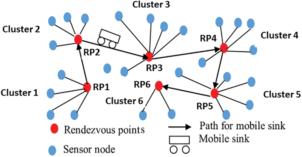
Figure 1: Mobile sink based WSN architecture

The RP-based path approach mitigates the issue of prolonged MS paths, thereby minimizing the complexity of data delivery. Nevertheless, designing the MS path presents a complex challenge as it significantly affects network coverage, data delivery efficiency, and network lifespan. Achieving rapid data delivery requires minimizing the path length of the MS. However, it is essential to recognize that a shorter path length implies increased multi-hop communication, resulting in higher hop counts and longer multi-hop path lengths, ultimately leading to raised energy consumption by SNs. Extending the Mobile Sink’s (MS) trajectory entails a trade-off wherein the MS path length is optimized by reducing hop counts and shortening multi-hop path lengths.

Sensor networks operate with reserved batteries in sensor nodes. Each node transmits data within its communication range, which is affected due to battery depletion addressed in [18]. This is another major drawback of WSN. In [19], a hybrid optimized localization methodology is introduced for the precise localization of mobile nodes within Underwater Wireless Sensor Networks (UWSNs). Despite advancements, further enhancements are required to achieve expedited and efficient routing protocols, thereby augmenting the longevity and efficacy of Wireless Sensor Networks (WSNs) within the network infrastructure.

In this study, after addressing the limitations of WSN, we present two hybrid energy-efficient algorithms, “Reduced k-means based with Artificial Neural Network” (RkM-ANN) and “Delay Bound Reduced k-means with ANN” (DBRkM-ANN), to improve the design of Rendezvous Points (RPs) paths for Mobile Sink (MS). The proposed model initiates by generating a candidate set of positions through k-means clustering [20] applied to a set of Sensor Nodes (SNs). Subsequently, it contrasts this model with a hybrid approach employing both k-means clustering and Artificial Neural Network (ANN). After that, we optimize this set to ascertain the minimal number of RPs based on predefined criteria. Unlike RkM, DBRkM-ANN incorporates a delay-bound parameter when selecting RPs. RkM-ANN develops a speedy and more efficient MS path by decreasing overall hop counts and average hop distance, while DBRkM extends this optimization by also considering delay-bound constraints. All this methodology is again compared with the proposed DBRkM-ANN in order to make the system more effective. We conducted a comprehensive analysis of our proposed algorithms, comparing the results of RkM-ANN and DBRkM-ANN with traditional k-means-based [21] approaches, DBRkM [22] and WRP [23] algorithms. Our assessment encompasses number of hop counts, energy consumption of SNs, End-to-End delay, number of packets received to the base station and network lifetime.

Several research activities have explored the same issues. However, in contrast to prevailing methodologies, the proposed solutions incorporate two different parameters not included in existing schemes. Besides carefully selecting Rendezvous Points (RPs) characterized by the highest neighboring Sensor Nodes (SNs) and positioned close to the optimal distance range, the algorithms prioritize minimizing the overall number of hops. Moreover, they optimize the average hop distance between RPs and SNs to reduce the total transmission distance. In particular, none of the past studies have comprehensively addressed all these factors concurrently. Additionally, the study introduces an effective data collection strategy designed to successfully mitigate the buffer run-off challenge.

Contributions:

The key contributions of the study are summarized as follows:

•   This study proposed two novel hybrid energy-efficient algorithms, “Reduced k-means based with Artificial Neural Network” (RkM-ANN) and “Delay Bound Reduced k-means with ANN” (DBRkM-ANN), to improve the design of Rendezvous Points (RPs) paths for Mobile Sink (MS) to have more efficient WSN with less latency and the design of delay-bound paths the MS

•   A unique strategy for finding the shortest path to reach RPs is explored in the study by applying TSP methodology to overcome the revisit constraints of SNs.

•   This paper explores energy consumption, end-to-end delay and network lifetime of WSN which mainly emphasizes the importance of solving these problems for its efficiency.

•   The proposed approaches are powerful and enhanced versions. It decreases the energy consumption of SNs and prolongs WSN’s lifetime.

2  Literature Review

Several approaches aim to control Mobile Sink (MS) mobility for effective data gathering in Wireless Sensor Networks (WSNs) [24–28]. However, the management of MS mobility falls into two primary categories: Random mobility [9] and controlled mobility [10]. While random mobility implementations are straightforward, they introduce unnecessary delays in data gathering [29]. In contrast, controlled mobility schemes establish the MS path based on predefined points or specific locations, often referred to as Rendezvous Points (RPs) [30]. In past studies [31], researchers have encouraged planning a stationary MS path using RPs, with sensor nodes (SNs) randomly positioned in proximity to this path.

Sensor Nodes (SNs) are divided into two classes based on their proximity to the predefined path. The first class encompasses SNs within the communication range of the path; while the second class consists of the remaining SNs. SNs in the first class directly transmit data to the MS, while the second-class nodes relay their data through the first-class nodes. Nevertheless, these methods lack constraints on tour distance, rendering them unsuitable for delay-sensitive applications. In a study by Ghafoor et al. [7], the Hilbert curve was employed for designing an MS path in homogeneous Wireless Sensor Networks (WSNs). From this perspective, MS strictly approaches each SN, enabling one-hop communication for data gathering. However, this strategy results in a longer path, proving impractical for numerous critical applications.

Authors explain the method of multiple sinks following the predetermined routes in [32], but the Mobile Sink’s (MS) tour length, which is critical for reducing data transmission latency, is neglected. Specifically for path establishment during MS path designing, in [23], the authors present Weighted Rendezvous Planning (WRP), a delay-constrained technique, to address the issue. Based on the number of data packets provided and the sensor node’s proximity to the closest Rendezvous Point (RP), WRP distributes weights to each node. However, the approach is not suited for large-scale Wireless Sensor Networks (WSNs) due to its significant time complexity of O(n5), where ‘n’ is the total number of sensor nodes. A Cluster-Based (CB) approach is proposed in [33] that uses binary search to find the minimal amount of RPs needed. In [34], authors discussed three mobile ad-hoc proactive and reactive routing protocols named DSDV, AODV and DSR, that work on the routing tables which are maintained at each node and find a route to a destination on demand, whenever communication is needed but still carries complexity.

In contrast to previous strategies, the suggested method optimizes the path for mobile sinks (MS) by taking into consideration three extra parameters: Average hop distance, distance from the Maximum-Distance Data (MDD) point, and one-hop neighboring SNs. These parameters are considered to formulate an efficient MS path.

3  System Model

We are analyzing a homogeneous Wireless Sensor Network (WSN) configuration, where Sensor Nodes (SNs) are distributed randomly across the selected area. The Sink, or data collection point, is supposed to navigate the target region at a consistent rate. The physical constraints in this study are as follows:

(1)   After deployment, each node remains stationary and is uniquely identified by a distinct ID.

(2)   Nodes exhibit homogenous communication and processing capabilities, but heterogeneous battery energy levels.

(3)   Data aggregation is employed, compressing multiple data points into a single packet.

(4)   Nodes work under a control mode based on distance power, ensuring uniform operation.

(5)   The initial energy of nodes varies and is not rechargeable.

(6)   Communication links between nodes are symmetric, resulting in even energy consumption and data transmission rates between nodes.

We have made several additional assumptions for our study.

Communication Conditions: Nodes can establish communication with each other if they fall within their respective communication ranges. All communication occurs wirelessly.

Stationary SNs: Once deployed, the SNs remain fixed in their positions throughout their operational lifespan.

MS Break Time: MS Break Time is the time in which MS collects data from the designated RPs. In this study, we only assume that the MS break time is sufficient to gather data from the SNs effectively.

Network Functionality: The network is considered operational until a specific percentage of the total SNs have depleted their energy.

Energy Model: The same energy model as mentioned in [35] is adopted in this research. Furthermore, no data retransmissions methodology is assumed, and the transmission speed along MS’s path remains constant.

These assumptions serve as the foundational framework for our analysis of WSN’s behavior and performance under specific conditions.

3.1 Mathematical Modeling

In developing our algorithms, we use the following specialized terminology.

Center (CR): This point provides the primary center of reference within the selected area. The mean values of the x- and y-coordinates of the deployed SNs are used to determine their coordinates.

xCR=1n∑i=1nxi(1a)

where i = 1, 2, …, n

xCR shows the mean value of x-coordinates

yCR=1n∑i=1nyi(1b)

where i = 1, 2, …, n

yCR shows the mean value of y-coordinates.

Hop Distance (HD): It indicates how far an RP is from its nearest neighbor (nhi) over one hop.

Average Hop Distance (AHD): An RP’s AHD is calculated by averaging the hop distances of its nearest neighbors. The mathematical expression is given below:

AHDi=∑j=1|OHNi|dist(ci,nhj)|OHNi|(2)

where i and j = 1, 2, …, n

“OHN” represents one hope neighbor from position i to position j;

“nhj” represents nearest neighbor.

Desired Distance Range (DDR): A decrease in network lifetime because of selecting a route for an MS that is too distant or too close to the center of the target region. As a result, the MS’s route should be selected such that it is between the two extremes of the intended space. This distance is called the Desired Distance Range, which can be written mathematically as

DDR=∑i=1ldist(CR,EPi)2l(3)

where, l indicates the number of extreme points.

4  Suggested Algorithms

The main concept of the suggested algorithms is outlined as. We initiate by acquiring a collection of possible Rendezvous Points (RPs) positions across the designated region of interest. To achieve this, we employ the k-means clustering algorithm [20] supported by the proposed ANN utilizing the spatial coordinates of the deployed Sensor Nodes (SNs). Subsequently, we aim to optimize this initial set of potential RPs. Our optimization objectives are as follows:

a. Practically make sure that every SN can be accessed with the least hop distance possible using one-hop communication.

b. The selection of RPs is such that it should not be too distant from or extremely close to the center of the targeted area.

This methodology is constructed on the utilization of a weight function, which is formulated through the following procedure.

4.1 K-Means Clustering Algorithm

This section explains the fundamental k-means clustering algorithm. Its objective is to partition a given dataset into a predetermined number, k, of non-overlapping clusters. The algorithm comprises two phases: Firstly, defining k centroids, each corresponding to a cluster, and subsequently assigning each data point to the nearest centroid based on Euclidean distance. Upon completing the initial grouping, centroids are recalculated to accommodate potential shifts due to newly included points. This iterative process continues until centroids stabilize, indicating convergence.

The k-means algorithm is widely researched and often yields satisfactory clustering outcomes. However, its primary drawback lies in the sensitivity to initial centroid values, leading to varied cluster formations. The algorithm’s computational complexity is notable, scaling proportionally with the product of data items, clusters, and iterations.

4.2 Weight Function

In this article, a weight function, Wt(i) is created, by carefully considering several factors that determine whether the possible location is appropriate for a rendezvous point (RP). The following is a description of these parameters:

i) One-Hop Neighbors to a Potential RP Position: To achieve comprehensive coverage of all Sensor Nodes (SNs) while minimizing the count of RPs, it is imperative that each RP covers a substantial number of neighboring SNs. Therefore,

Wt(i)∝|OHNi|(4)

ii) Distance to Desired Distance Range (DDR): Experimental observation reveals that augmenting the parting between RP and DDR correlates with a rise in hop counts. Therefore, prioritizing the reduction of this distance is imperative.

Wt(i)∝1mod(DDR−disr(CR,ci))(5)

where i = 1, 2, …, n

iii) Average Hop Distance: The energy consumed during the transmission of a data packet is directly linked to the transmission distance, following a power-law relationship where 2 < α < 4. Therefore,

Wt(i)∝1AHDi(6)

where i = 1, 2, …, n

Relating all the parameters explained from Eqs. (4) to (6), we get

Wt(i)=Z∗|OHNi|mod(DDR−dist(CR,ci))∗AHDi(7)

where “Z” represents proportionality constant, considering Z = 1. We get

Wt(i)=|OHNi|mod(DDR−dist(CR,ci))∗AHDi(8)

It is essential to note that within the weight function Wt(i), these parameters are interconnected, with each potentially influencing the others. This interdependency arises due to the variation of these parameters across different value ranges. Consequently, to facilitate a consistent assessment, we normalize each parameter within the range of 0 to 1, employing the following methodology.

OHNi  ′=|OHNi|max(|OHN|)(9)

AHDi  ′=|AHDi|max(AHD)(10)

DDRi  ′=mod(DDR−dist(CR,ci))max(mod(DDR−dist(CR,cj)))(11)

Wt(i)=OHNi  ′DDRi  ′∗AHDi  ′(12)

4.3 Proposed Artificial Neural Network (ANN) Algorithm

One type of Artificial Intelligence is Machine Learning (ML) and Artificial Neural Networks (ANNs) is a subfield of ML. The human brain’s biological neural networks serve as the inspiration for ANNs, which are computer models. The “neurons” of an ANN are just like the nodes in a network, and they process and send data. Energy prediction, data analysis, and decision-making are just some of the many uses for ANNs, many of which are used in WSNs [36].

ANNs are made up of nodes that are interconnected, called neurons that are arranged in layers. Each neuron processes inputs and produces an output using weighted connections and activation functions. Predictions are made based on the patterns and correlations they learn from trained data.

There are two primary types of Artificial Neural Network (ANN) learning approaches called supervised and unsupervised [37]. In this research, supervised ANN learning architecture is applied on WSN as shown in Fig. 2. A total of fifty Wireless Sensor Networks (WSNs) in which each network contains sixty-four Sensor Nodes (SNs) called clusters. Each cluster contains one Cluster Head (CH) node containing the highest energy level that collects information from all the other nodes and forwards it to the next CH node of another cluster network, and at the end the final data is transferred to the Base Station (BS), which is using the architecture of ANN as a single-layer feed forward neural network containing three layers. First is the input layers, second are one or more hidden layers and the third one is the output layer on each cluster.

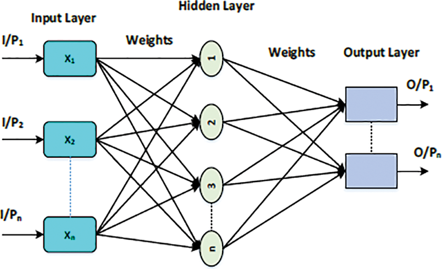
Figure 2: Supervised learning ANN architecture [37]

4.3.1 Mathematical Modeling of ANNs

The mathematical equations governing the functioning of a feed forward neural network can be described as follows:

Input Layer

The input layer, also called Layer 1, consists of input features denoted as xi (where i = 1, 2,..., n). The input layer has n neurons, each representing one feature. The output of the ith neuron in the input layer (denoted as ai(0)) is just the input feature itself. In this case, we have taken into account a hundered input layers and sixty-four neurans per layer.

Hidden Layer

The hidden layer consists of m neurons, where m is the number of hidden units. Each neuron in this layer takes inputs from the input layer and produces an output using weighted connections (wi(1j)) and an activation function (g). The output of the jth neuron in the hidden layer (aj(1)) is calculated as follows:

aj(1)=g(∑i=1n(wi(1j)∗ai(0)+bj(1)))(13)

where:

wi(1j)∗ai(0)+bj(1) is the output of the jth neuron in the hidden layer.

wi(1j) is the weight connecting the ith input feature to the jth neuron in the hidden layer.

ai(0) is the output of the ith neuron in the input layer.

bj(1) is the bias term for the jth neuron in the hidden layer.

Output Layer

Layer 3, indicated as the output layer, comprises k neurons, where k indicates the number of output classes or regression outputs. Analogous to the hidden layer, each neuron within the output layer takes inputs from Layer 1 and produces an output utilizing weighted connections (wj(2k)) and an activation function (g).

The ending result of the kth neuron in the output layer (ys) is calculated as follows:

ys=h(∑j=1m(wj(2s)∗aj(1)+bs(2)))(14)

where:

ys stands for the output of the kth neuron in the output layer (which represents the final anticipated outcome of the neural network’s output layer.).

wj(2s) shows the weight that connect the jth neuron in the hidden layer to the kth neuron in the output layer.

aj(1) denotes the output of the j-th neuron in the hidden layer.

bs(2) represents the bias term associated with the k-th neuron in the output layer.

g shows the activation function applied element-wise to the weighted sum of inputs and biases.

The overall processing of forward propagation through the neural network involves calculating the output of each layer, in which the input layer working is initialized and proceeding through the hidden layer(s) to the output layer. The expected output result (ys) is then compared to the actual output during the training process to compute the loss, weights and biases are updated using an optimization algorithm to lessen the loss and increase the network’s performance. This is known as back propagation, and it is used to adjust the network’s parameters iteratively during training to learn meaningful representations and make accurate predictions.

Neuron Activation

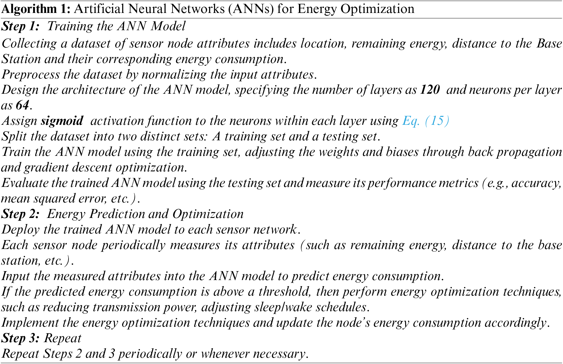
The activation of a neuron in an ANN can be calculated using an activation function and in this study we are using the sigmoid function:

Activation=11+exp−z(15)

Here, z represents the weighted sum of inputs to the neuron.

Wireless Sensor Networks (WSNs) often utilize AI algorithms for routing to optimize data transmission, reduce energy consumption, and improve network efficiency. In this paper, ANN is used as an AI-based routing algorithm for WSNs. ANNs are part of the broader category of machine learning algorithms and are used in Wireless Sensor Networks (WSNs) for routing by employing them as intelligent decision-making components to determine the most suitable routing paths based on network conditions. Here’s how we applied ANN algorithms in WSN routing.

1.   Data Collection and Feature Extraction:

We gather data about WSN, including information about the network topology, node status, node locations, energy levels, signal strengths, and historical routing data. After that, we preprocess and transform the data into a format suitable for input to the ANN.

2.   Applied Supervised Learning method:

In this research we used supervised learning setup, labeling the data instances with the desired routing outcomes. These labels represent the optimal routing paths or strategies.

3.   Data Preprocessing:

Preprocess the data and then feeding into the ANN. This involved scaling features, handling missing data, and splitting the data into training and testing sets.

4.   ANN Architecture Design:

The structure of the ANN is then determined. A total of one hundred and twenty input layers are used in this article, and then the number of neurons in each layer is initially considered as sixty-four, and sigmoid as the choice of activation function.

The input layer typically receives data on network conditions, and the output layer provides routing decisions. The intermediate hidden layers process this information.

5.   Training the ANN:

Train the ANN using the labeled data. During training, the network adjusts its internal parameters (weights and biases) using equations Eqs. 13 and 14to minimize the error between predicted routing paths and the labeled paths. The network learns to make routing decisions based on the input data and the labeled outcomes.

6.   Routing Decision:

When a data packet needs to be transmitted from a source node to a destination node, the trained ANN is used to make a routing decision. Input to the ANN includes current network conditions, such as node locations, energy levels.

The output of the ANN is a routing decision, specifying the next hop or set of nodes through which the data packet should be forwarded.

7.   Data Transmission:

The data packet is transmitted through the nodes determined by the ANN’s routing decision.

8.   Feedback and Learning:

After data transmission, the ANN receives feedback on the success or failure of the routing decision. This feedback is used to update the ANN’s parameters during online learning, which further refines its routing decision-making capability.

The proposed ANN architecture system is trained based on the energy consumption and delay of the nodes. We have pre-trained the ANN model based on a data set that includes the total number of nodes in the network, which is three hundred, the initial energy of each sensor node and intra node distance and each node’s threshold energy. Fig. 3 shows the trained structure of ANN with Mean Square Error (MSE). If a node’s communication energy delay falls below the specified threshold, it is considered as a failed node. The system then selects a nearby node as a replacement communication node, integrating it into the communication path. Among the 64 contributing neurons, representing node properties such as energy and delay, inputs are given into the ANN’s input layer. With a hidden layer comprising ten neurons, optimal performance is achieved. The output layer consists of 56 neurons, indicating eight failed nodes out of the original 64, demanding removal from the network. This approach saves node energy, thereby extending network lifespan.

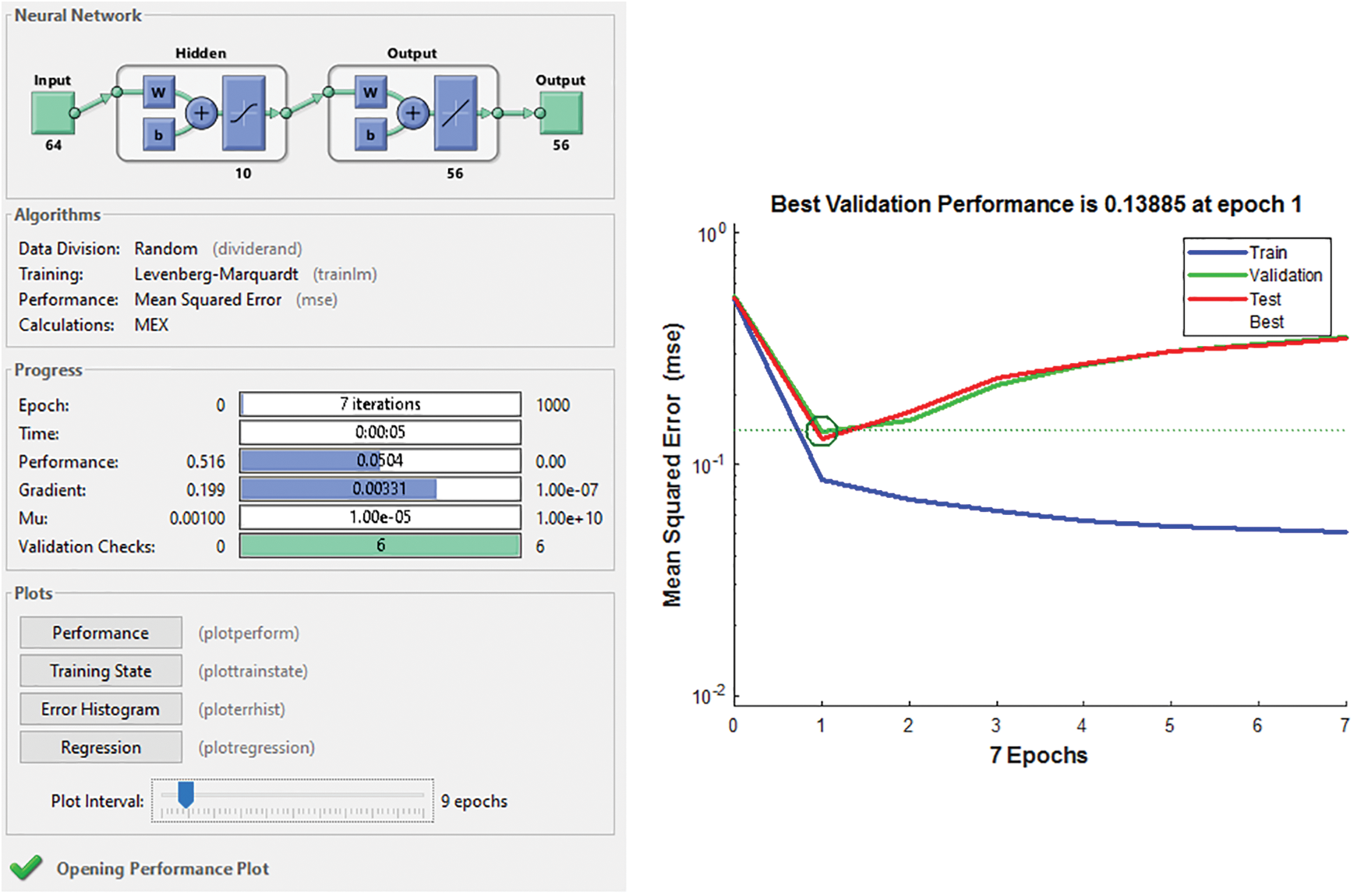
Figure 3: Trained ANN structure

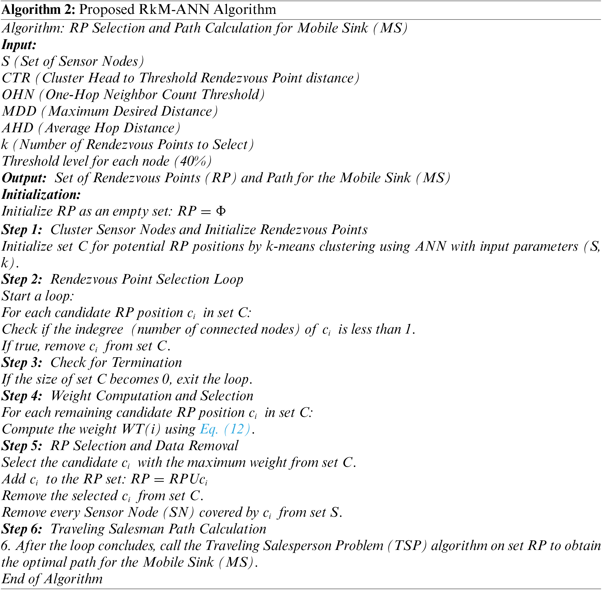
4.4 Proposed RkM-ANN Algorithm

We initiate the process by initializing the set of potential positions for Rendezvous Points (RPs), denoted as C, through k-means clustering algorithm using ANN. Subsequently, our primary objective is to minimize the count of potential RP positions while ensuring the coverage of every Sensor Node (SN) within a single hop communication range, thus optimizing hop distance and conserving energy.

To achieve this, we employ the Reduced k-means hybrid with the ANN (RkM-ANN) algorithm, which operates as follows:

a. During the iteration process of RkM-ANN, we systematically eliminate any potential RP position that covers at most one SN. This strategic elimination is geared toward energy conservation.

b. Next, we calculate the weight of the remaining potential RP positions, subsequently selecting the one with the highest weight value.

c. The chosen RP and all SNs covered by it, is then removed from consideration.

d. This iterative process remains continued until the set C becomes empty.

e. After the creation of the final set of RP placements, we used Christofides’s heuristic to support the proposed method using the Traveling Salesman Problem (TSP) [38] algorithm to find the best route for the Mobile Sink (MS).

Using TSP, this algorithm determines the best possible route for the Mobile Sink by continually selecting Rendezvous Points from a candidate set according to specified criteria.

Theorem 1: The RkM-ANN algorithm exhibits a time complexity of O(nkl + kt + kn +k3), where n is the number of nodes, k is the desired number of Rendezvous Points (RPs), p represents the dimensions in k-means clustering, t denotes the count of remaining potential RP positions, and q signifies the selected number of RPs.

Proof:

1. Initialization of an empty set RP in Step 1 invites constant time.

2. Utilizing the k-means clustering algorithm with ANN to attain potential RP positions in Step 2 requires O(nkpl) time.

3. Steps 3 to 6, involving the selection of q RPs, consume O(mt + mn) time, where “t” represents the remaining count of k’s (potential RP positions).

4. Using Christofis’s heuristic method in O(m3) time the k positions utilize to compute the MS path.

5. Consequently, the overall time complexity of the RkM-ANN algorithm is expressed as O(nkl + mt + mn +k3). For worst-case scenario, when the number of RPs =(k), the time complexity becomes O(nkl + kt + kn +k3).

Explanation:

RkM-ANN establishes one-hop communication for equal Sensor Nodes (SNs) distribution. Simulation results indicate that 96% of SNs lie within a one-hop distance of the selected Rendezvous Points (RPs), even in unequal deployments. The remaining 4% of SNs achieve RP connectivity within 2 or 3 hops through intermediary SNs. While RkM-ANN confirms energy-efficient Mobile Sink path formation, it lacks a guarantee for data delivery within a specified delay, a critical constraint for real-time applications. This constraint is addressed by the subsequent DBRkM-ANN algorithm, detailed below.

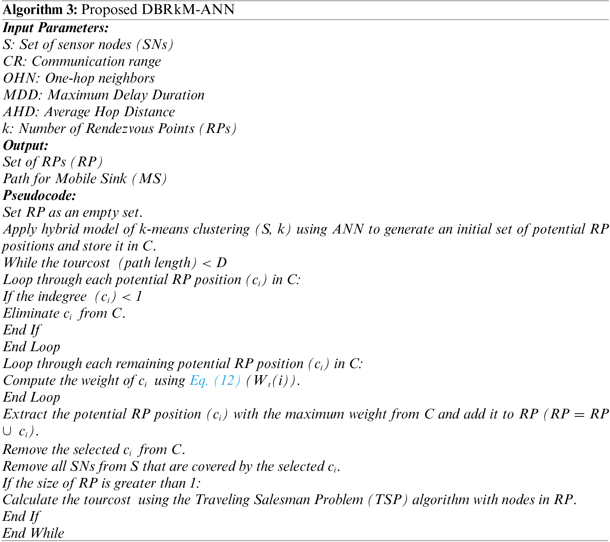
4.5 Proposed DBRkM-ANN Algorithm

The key objective of the proposed hybrid model is to search for a minimalized set of Rendezvous Points (RPs) that allow the Mobile Sink (MS) to gather information efficiently within a sufficient latency, reducing hop counts and distances for energy management. Similar to RkM-ANN, DBRkM-ANN begins with a k-means clustering with an ANN predefined set of potential RP positions. The algorithm initializes an empty set of RP and iteratively chooses a potential RP position with the largest weight to add to the set. Afterward, the Traveling Salesman Problem (TSP) algorithm [38] determines the shortest path. The algorithm iterates until the path length crosses the predefined delay limit. The pseudocode for this approach is presented below:

Theorem 2: The DBRkM-ANN algorithm shows a time complexity of O(nkl + mt + mn +m4).

Proof:

1. Initialization of an empty set RP in Step 1 incurs constant time.

2. Obtaining k potential RP positions using k-means clustering using ANN in Step 2 requires O(nkl) time.

3. Steps 3 to 18 iterate q times to select q RPs, involving the removal of SNs covered by the selected RP and subsequent application of the TSP algorithm [38] to determine the path through the set RP.

4. Equation O(nkl + mt + mn +m4) expresses the overall time complexity of DBRkM-ANN. In the worst-case condition, when the selected RPs =k then, the new time complexity is O(nkl + kt + kn +k4).

Explanation:

This procedure initiates an empty set of RPs and generates an initial set of possible RP places using k-means clustering using ANN.

Based on specified requirements, continuously picks possible RP places, calculates their weights, and adds them to the RP set. SNs covered by selected RPs are removed from the SN set S.

The algorithm keeps executing until the tourcost (path length) is higher than its maximum delay duration (MDD).

Furthermore, using the nodes in RP, the TSP method is used to determine the Mobile Sink (MS) path.

Note: The following pseudocode is based on the availability of specific functions (e.g., TSP, Eq. (12), and indegree).

4.6 Proposed Data Gathering Scheme

4.6.1 Data Gathering and Communication Process

The Mobile Sink (MS) chooses a destination RP for each Sensor Node (SN) based on its corresponding distances after selecting the Rendezvous Points (RPs). The decision of the nearest RP for each SN is important in order to ensure uniform energy distribution across the network. Following this assignment, MS initiates the broadcast Information Packet for the Rendezvous Points (IPR) to the whole network, encapsulating crucial information.

Upon reception of the IRP, SNs take its contents to establish their respective destination RP. With this information in hand, all SNs are now ready to transmit data to their designated RPs. The data gathering period is organized into different rounds, each involving the MS’s traversal of the selected area to collect information. The MS sequentially visits the selected RPs for data retrieval from the SNs.

When SN falls within the communication range of its designated RP, it directly forwards its data to the MS. Conversely, if the distance requires, the SN utilizes its nearest SN as a relay to facilitate data transmission to the RP. As the MS approaches a specific RP, it issues a polling message, denoting the RP’s identifier. SNs intend to transmit data through when the data arrives at the RP, which then processes the received data and sends it to MS.

This process will continue until MS has successfully collected information from all the SNs assigned to each RP; after that, it moves on to the next RP. Each SN is only responsible for saving its own data using its own buffer, and this is one of the main advantages of suggested techniques. In comparison, information is kept in Data Storing Nodes (DSNs) that are one hop away from the RP in the traditional data collection architecture [39]. With the second approach, nodes that are two or more hops distant from DSNs have to relay their data to them, which enhances the possibility of data overflow, which can lead to data loss and retransmission.

4.7 Traveling Salesman Problem (TSP) Mechanism

The TSP involves the returning mechanism of a salesman looking for the smallest route to find food from specified cities, and then returning to their initial city. For mathematical representation, one can use the entire weighted graph G=(N,A)G=(N,A), where N shows the number of nodes that stand for cities and A is the set of arcs that totally connect with N. The length of each arc, denoted by the symbol dxy, is measured in units of this kind (x; y). TSP involves determining the minimum possible Euclidean distance between any two nodes in the graph G. With symmetric TSPs, the distance between any two cities called nodes, denoted by dxy, is equal to dyx regardless of which way the arcs are traversed.

5  Experimental Results

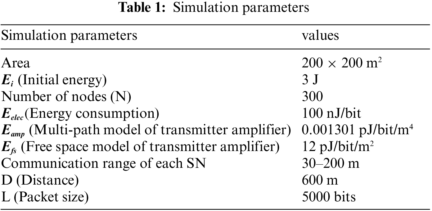
The proposed algorithms are carefully evaluated through simulations conducted on Matlab software (R2021a version) on Windows 8.1. The system employed for these simulations was equipped with 8 GB of RAM and featured a processor running at 2.5 GHz, housing an Intel Core i-7 CPU. The assessment of these algorithms encompassed a range of network scenarios achieved by varying the number of Sensor Nodes (SNs) across a target area measuring 200 × 200 square meter (m2). Each SN was initially endowed with 3 Joules (J) of energy, and no energy limitations were imposed on the Mobile Sink (MS). The MS was assumed to move at a velocity of 4 m/s. The parameters investigated in this study are mentioned in Table 1. In our analysis, we compared the RkM-ANN algorithm with a technique that generates q RP positions directly using straightforward k-means clustering using ANN, the traditional RkM [22] and K-means based algorithms. Furthermore, DBRkM-ANN was compared with two existing algorithms, namely the traditional DBRkM [22] technique and Weighted Rendezvous Planning (WRP) [23].

The results of these simulations were subjected to a comprehensive evaluation utilizing multiple performance metrics.

5.1 Result and Analysis of RkM-ANN

The Figs. 4 and 5 show the runtime scenarios of both the k-means-based ANN and RkM-ANN approaches. These scenarios were generated using a network configuration consisting of 20 Sensor Nodes (SNs) with a communication range denoted as “r” equal to 50 meters (m). In the graphical representations, the data broadcast pathways by the SNs convey their detected data to the Rendezvous Points (RPs) are mentioned with the green lines, while the purple dash line illustrates the trajectory of the Mobile Sink (MS) to the RPs and the purple lines represent the connection path between the WSNs. It is important to note that this runtime scenario is visualized within a target area measuring 120 by 100 square meters (m2).

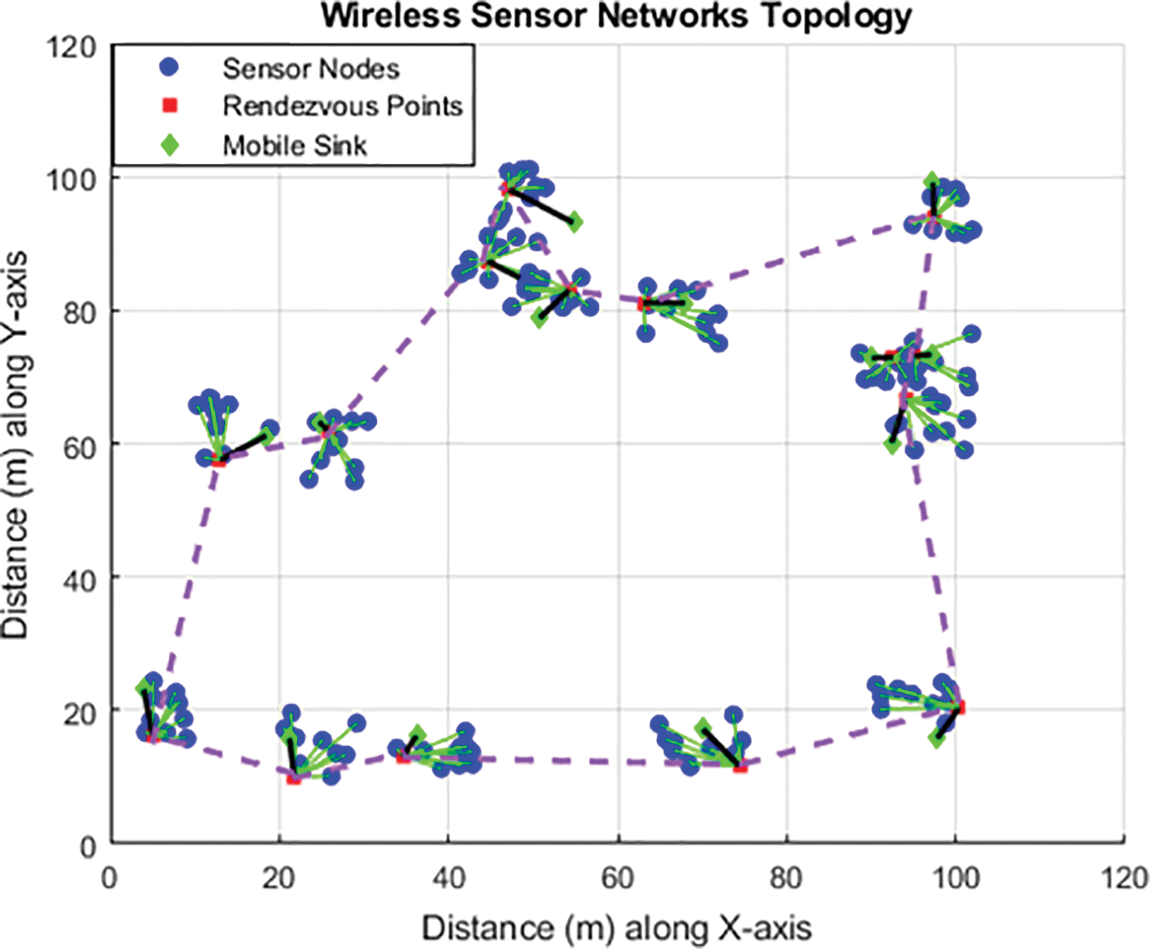
Figure 4: Experimental scenario of k-means based-ANN approach

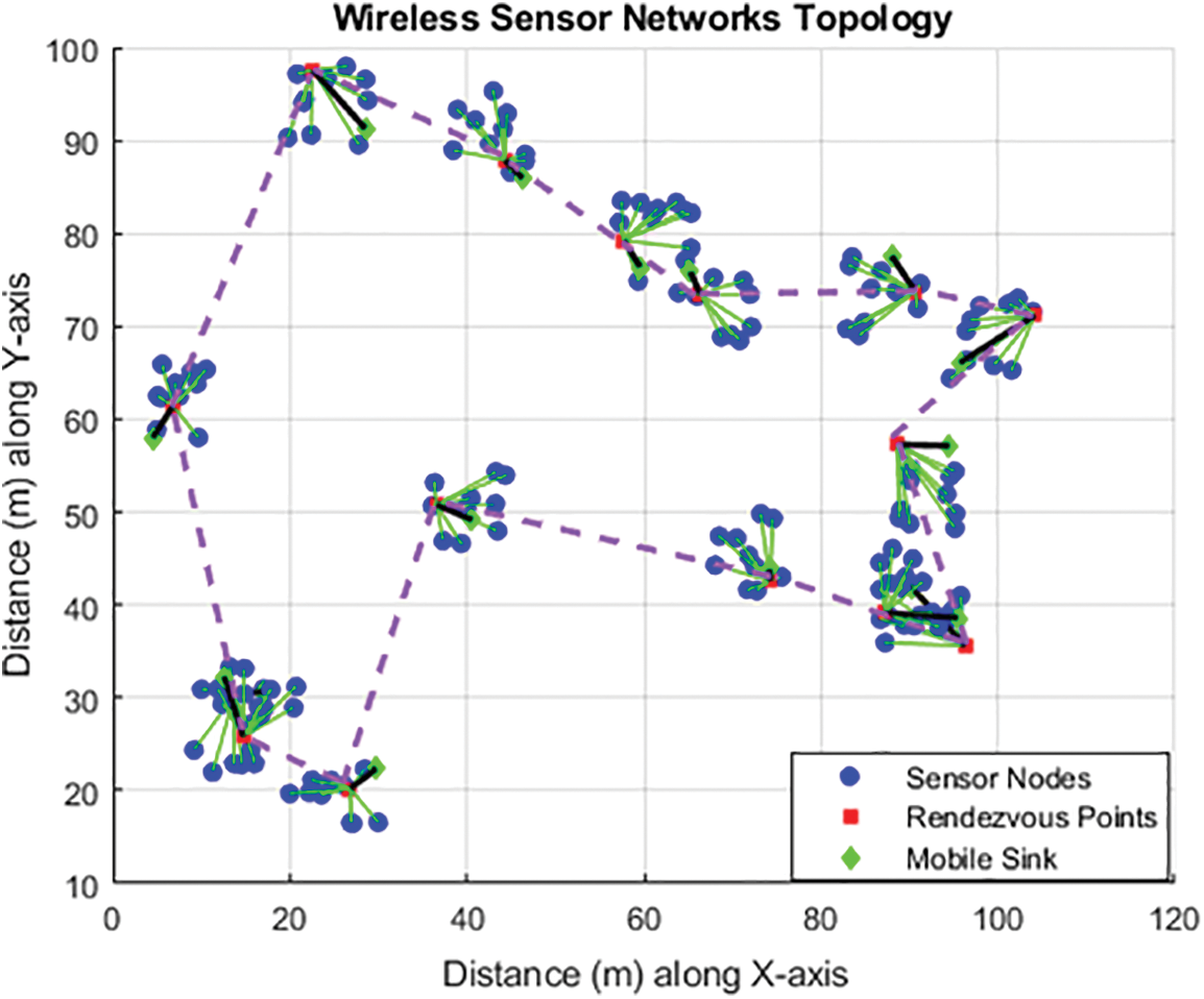
Figure 5: Experimental scenario of RkM-ANN approach

5.1.1 Analysis of Hop Counts

Fig. 6 represents the performance analysis of total hop counts under varying node densities for the clustering techniques of K-means based, proposed K-means based-ANN, Reduced k-means (RkM), and proposed Reduced k-means with ANN (RkM-ANN). The figure vividly illustrates that approximately 96% of SNs are protected by designated RPs. This outcome is attributed to the algorithm’s avoidance of RP placements covering only a single SN, resulting in about 4% of SNs communicating with MS through intermediary SNs. Notably, the total hop counts are significantly reduced in comparison to the simple k-means based approach with the proposed k-means-based-ANN algorithm model. In another proposed technique, RkM-ANN, potential RP positions with a higher number of one-hop neighbors are prioritized in comparison to the simple RkM approach.

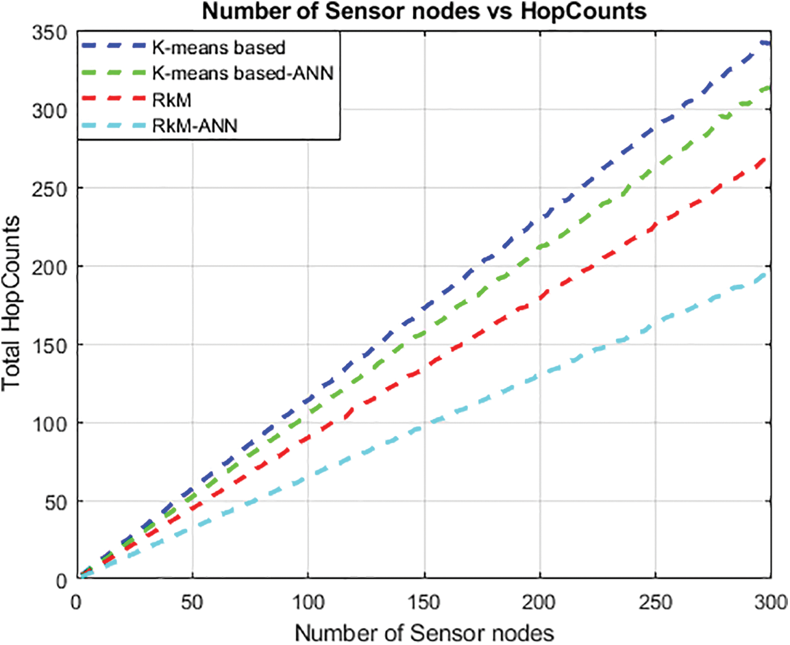
Figure 6: Number of sensor nodes vs. Number of hope counts

5.1.2 Analysis of Packets Received to BS

Fig. 7 presents the total received packets to the base station (BS), demonstrating that RkM-ANN outperforms the k-means based and k-means based-ANN and traditional RkM approach.

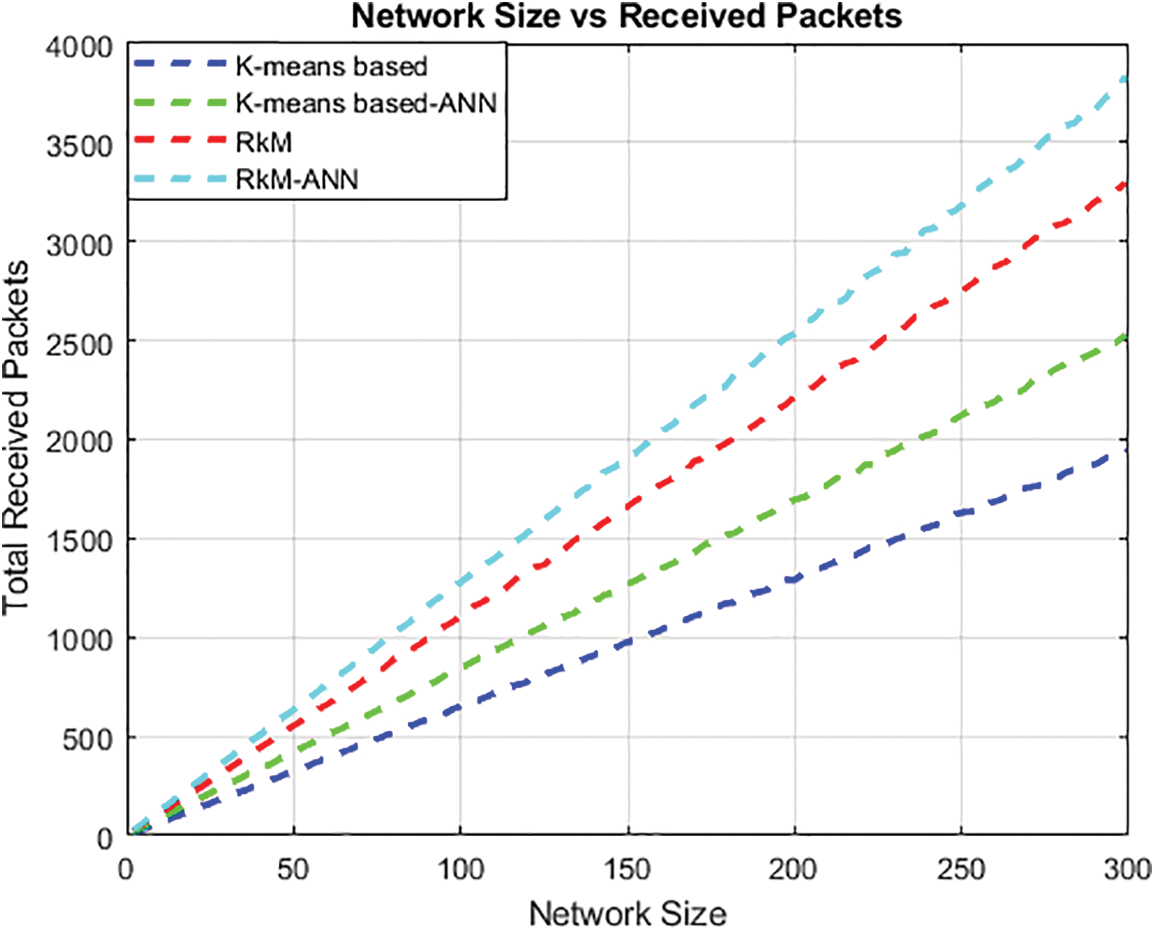
Figure 7: Network size vs. Received packets

5.1.3 Analysis of Energy Consumption

Fig. 8 showcases the algorithms’ performance in terms of energy consumption over various data collection rounds. Remarkably, RkM-ANN exhibits lower energy consumption than the RkM approach compared to the k-means-based and k-means-based-ANN approach.

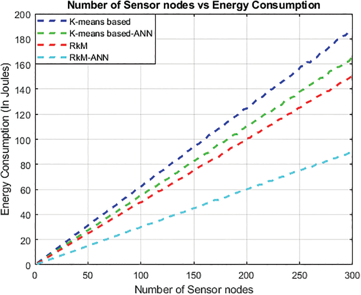
Figure 8: Number of sensor nodes vs. Energy consumption

5.1.4 Analysis of End-to-End Delay

Fig. 9 illustrates the comparison between RkM-ANN, RkM, k-means based and k-means based-ANN concerning the total number of End-to-End delays. It is evident that RkM-ANN outperforms the other three algorithms. This superiority can be attributed to the usefulness of the suggested weight function, which strongly emphasizes the reduction of End-to-End delay by choosing potential RPs with the highest indegree.

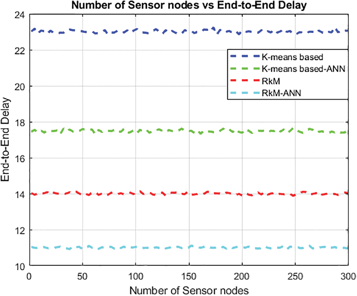
Figure 9: Number of sensor nodes vs. End-to-end delay

5.1.5 Network Lifetime

The proposed technique intensely increased the network lifetime under varying node densities through the weight function. The program optimized the routing patterns based on the expected energy consumption, leading to effective data transfer. This was achieved with the use of the RkM-ANN algorithm. This enhancement provided consistent data collection and decreased network wide data loss. Fig. 10 represents the graphical analysis of network size vs. network lifetime.

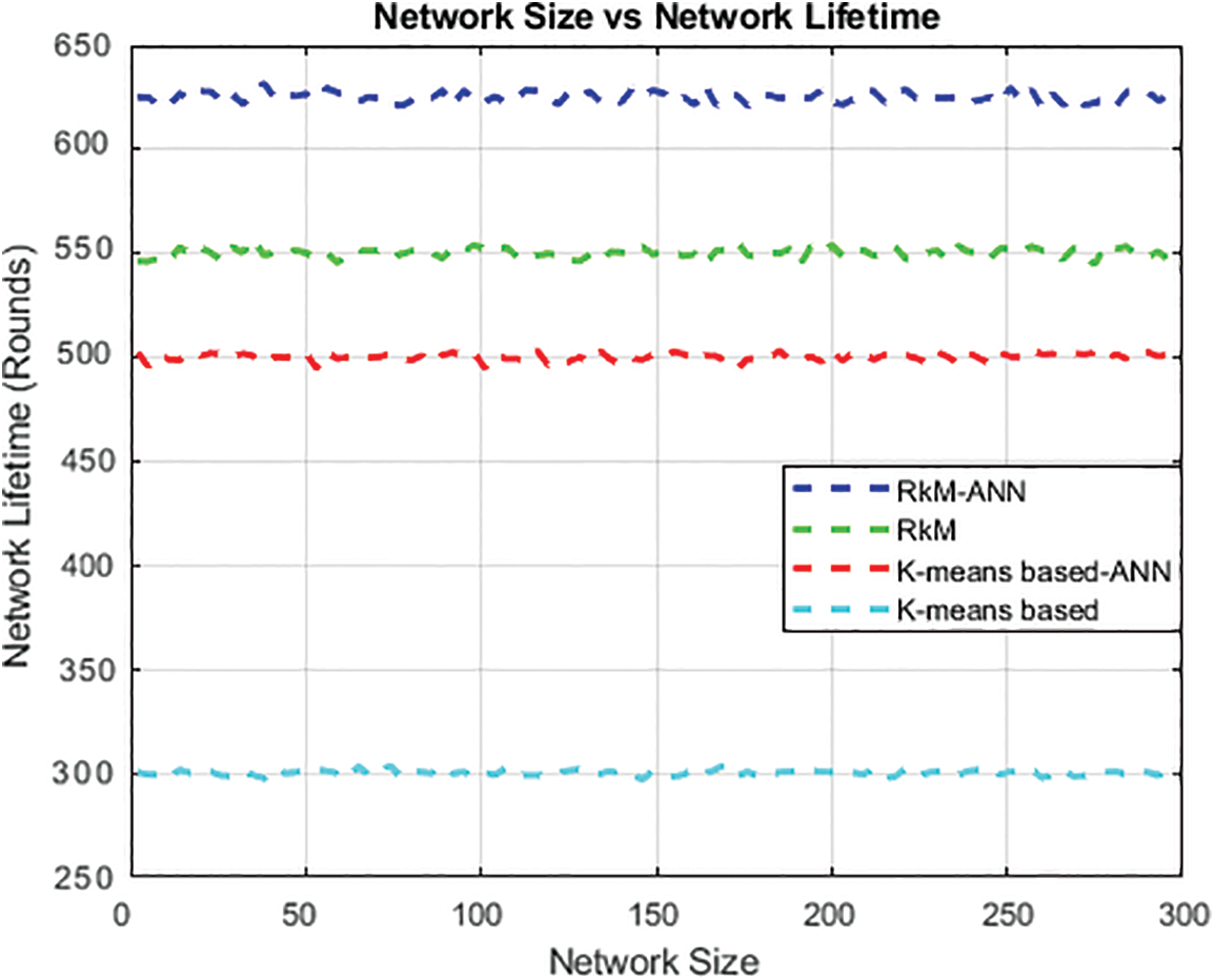
Figure 10: Network size vs. Network lifetime

5.2 Results and Analysis of DBRkM-ANN

In this section, different results are analyzed for different parameters that are taken into account in this article. They are given below.

5.2.1 Total Hop Counts

A comparison of total hop counts between DBRkM, WRP, and the proposed DBRkM-ANN is shown in Fig. 11. DBRkM performs better, which is explained by the effectiveness of the proposed weight function. Eq. (4) illustrates the function’s priority of reducing total hop counts through the selection of possible Rendezvous Points (RPs) with the highest indegree.

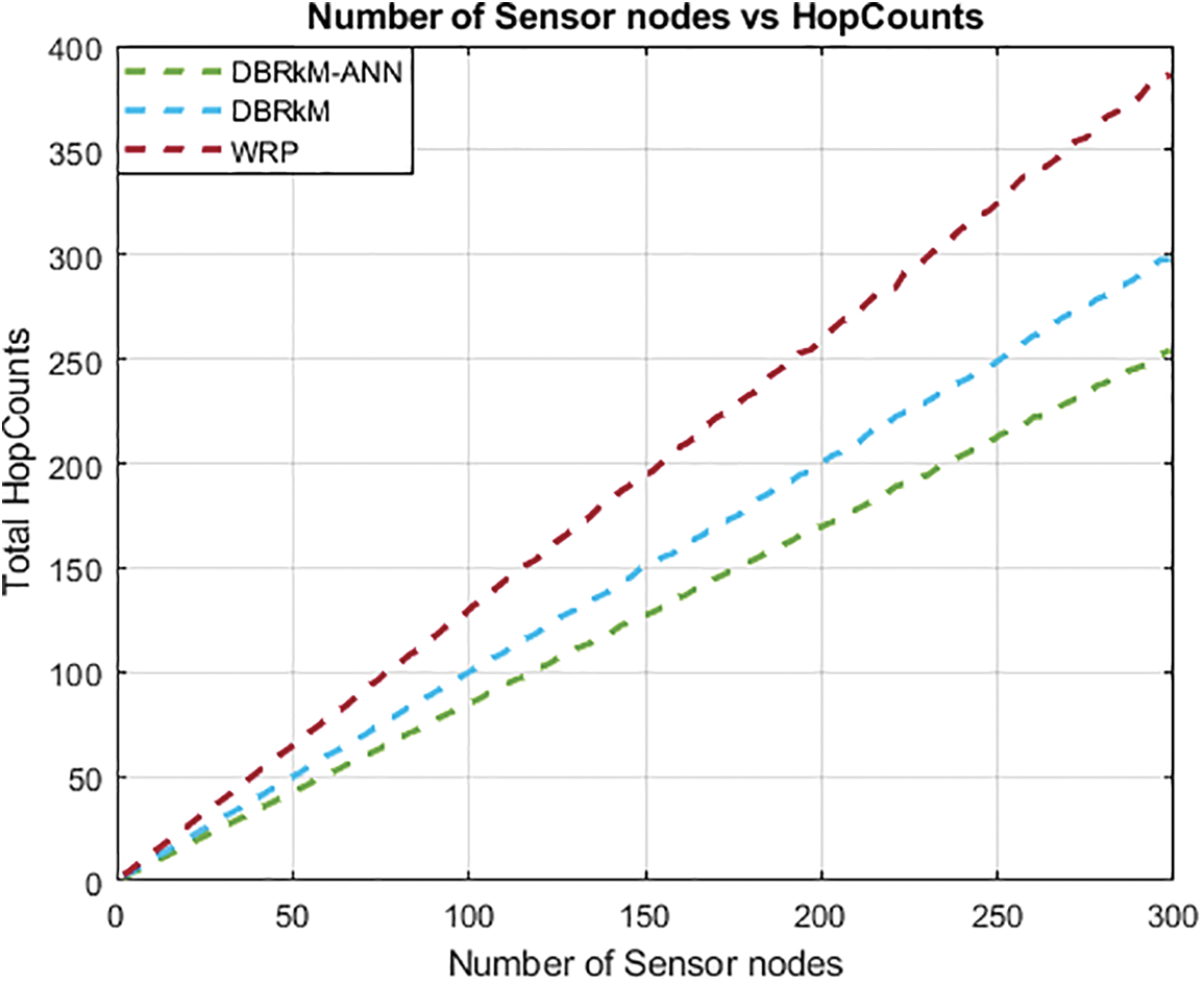
Figure 11: Number of sensor nodes vs. Hope counts

5.2.2 Analysis of End-to-End Delays

The number of End-to-End Delays is plotted in Fig. 12, showcasing DBRkM-ANN’s superiority over other algorithms. The proposed methodology has a lower number of End-to-End Delays in comparison with the other existing techniques.

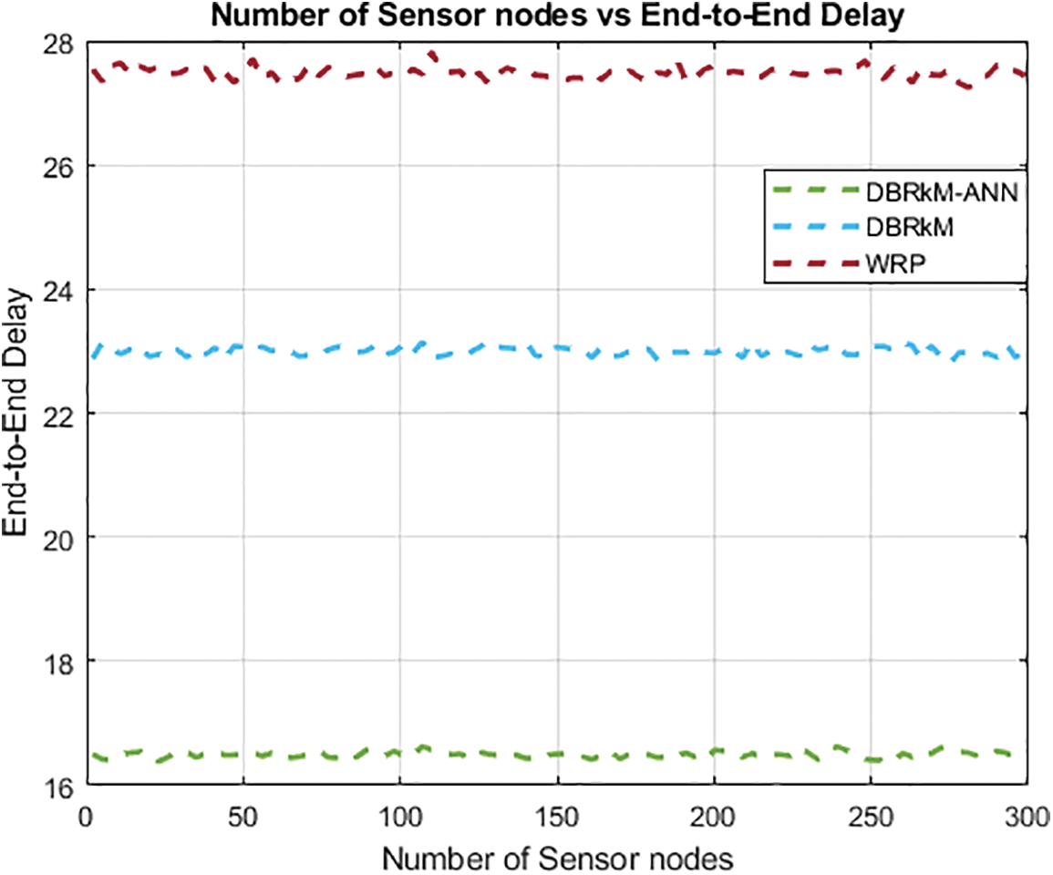
Figure 12: Number of sensor nodes vs. End-to-end delay

5.2.3 Analysis of Total Received Packets

Fig. 13 demonstrates the analysis of the proposed model DBRkM-ANN regarding the number of received packets. The results indicate that the suggested technique performs better than the other two algorithms in terms of the highest number of received packets.

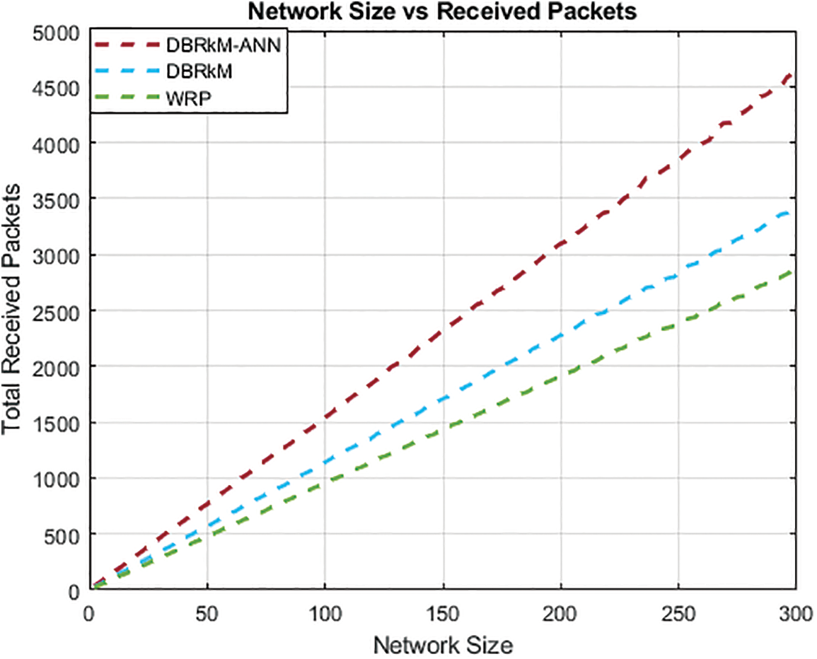
Figure 13: Network size vs. Received packets

5.2.4 Energy Consumption

The random deployment of 300 SNs in one single network as shown in Fig. 14. The energy of the network drops immediately as the data transmission initializes within the network. In this research, we have suggested the initial energy of the network is 3-Joules. According to the results after analysis, the network’s energy usage rose in tandem with progress. However, less energy consumption was noted by reducing multi-hop route lengths and the number of hops is counted when the hybrid approach. The DBRkM-ANN strategy was applied on WSN. As a result of the optimization of the network, less amount of energy was consumed than in the case of the other existing methodologies.

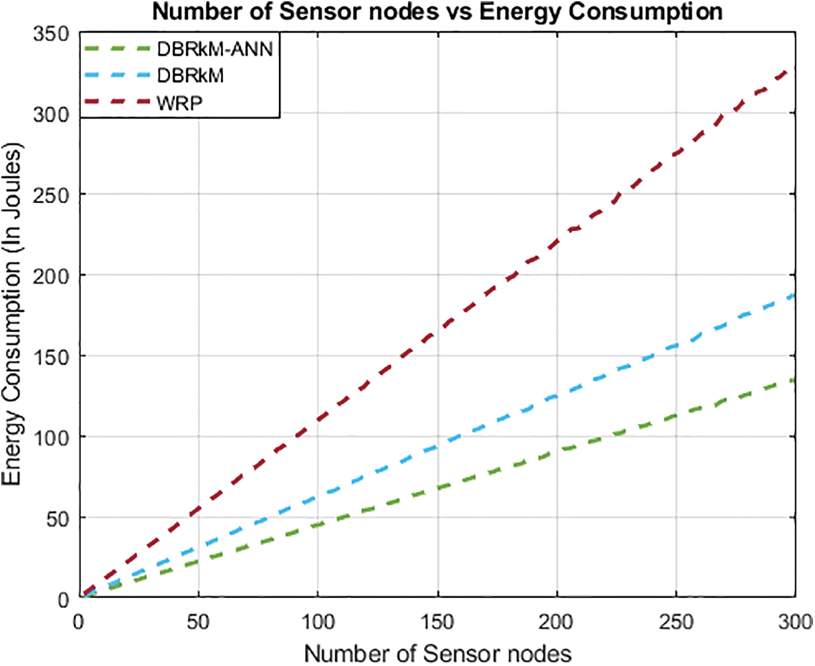
Figure 14: Number of sensor nodes vs. Energy consumption

5.2.5 Network Lifetime

The proposed technique “DBRkM-ANN” intensely increased the network lifetime under varying node densities through the weight function when compared with WRP and traditional BDRkM algorithms. The program optimized the routing patterns based on the expected energy consumption, leading to effective data transfer. This enhancement provided consistent data collection and decreased network wide data loss. Fig. 15 represents the graphical analysis of network size vs. network lifetime.

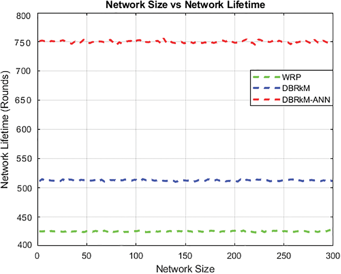
Figure 15: Network size vs. Network lifetime

6  Conclusion

This paper presents two novel hybrid algorithms, namely RkM-ANN and DBRkM-ANN, designed for the optimization of mobile sink (MS) and improved path formation within Wireless Sensor Networks (WSNs). Both algorithms are planned to facilitate efficient MS path selection by taking into account a multitude of critical factors. These factors encompass the maximization of one-hop neighbors, reduction of average hop distance, and minimization of the distance between Rendezvous Points (RPs) and the most favorable distance from a reference point. While RkM-ANN establishes a path via one-hop communication, DBRkM-ANN employs a similar technique to construct a path while adhering to delay-bound constraints. Both algorithms are rigorously evaluated against existing counterparts, namely Weighted Rendezvous Planning WRP and traditional DBRkM algorithms. Another strategy for finding the shortest path to reach RPs is investigated in the study by applying TSP methodology to mitigate the revisit constraints of SNs across networks. The assessment encompasses various performance metrics, including the total number of hop counts, energy consumption, and the number of received packets, end-to-end delay and network lifetime. The results conclusively demonstrate the superior performance of RkM-ANN and DBRkM-ANN across these metrics when compared to existing methodologies. In addition to path formation, this study presents a robust data gathering strategy intended for the mobile sink that will be used in every data collection cycle. This scheme is designed to minimize packet drops and enhance overall data collection efficiency. However, it is essential to acknowledge certain limitations in our work. We have assumed a uniform data generation load across all SNs, which might not hold true in practical scenarios where SNs exhibit varying data generation rates. Additionally, our work assumes negligible break time for MS. Addressing these limitations represents a potential avenue for future research, where efforts can be directed toward accommodating non-uniform data generation and exploring the implications of more realistic sojourn time scenarios.

Acknowledgement: The authors would like to thank the anonymous reviewers for their valuable comments.

Funding Statement: This work was supported by Research Supporting Project Number (RSP2024R421), King Saud University, Riyadh, Saudi Arabia.

Author Contributions: The authors confirm contribution to the paper as follows: Study conception and design: Muhammad Salman Qamar; data collection: Muhammad Fahad Munir; analysis and interpretation of results: Ihsan ul Haq, Amil Daraz; draft manuscript preparation: Atif M. Alamri, Salman A. AlQahtani. All authors reviewed the results and approved the final version of the manuscript.

Availability of Data and Materials: Not applicable.

Conflicts of Interest: The authors declare that they have no conflicts of interest to report regarding the present study.

References

1. M. S. Manshahia, “Wireless sensor networks: a survey,” Int. J. Scientif. Eng. Res., vol. 7, no. 4, pp. 710–716, 2016. [Google Scholar]

2. E. Ghorbani Dehkordi, and H. Barati, “Cluster based routing method using mobile sinks in wireless sensor network,” Int. J. Electron., vol. 110, no. 2, pp. 360–372, 2023. doi: 10.1080/00207217.2021.2025451. [Google Scholar] [CrossRef]

3. A. A. R. A. C. Omar and B. Soudan, “A comprehensive survey on detection of sinkhole attack in routing over low power and Lossy network for internet of things,” Internet of Things, vol. 22, pp. 100750, 2023. doi: 10.1016/j.iot.2023.100750. [Google Scholar] [CrossRef]

4. P. Shanmugaraja, M. Bhardwaj, A. Mehbodniya, S. Vali, and P. C. S. Reddy, “An efficient clustered m-path sinkhole attack detection (MSAD) algorithm for wireless sensor networks,” Ad Hoc Sens. Wirl. Netw., vol. 55, pp. 1–22, 2023. [Google Scholar]

5. E. H. Houssein, M. R. Saad, A. A. Ali, and H. Shaban, “An efficient multi-objective gorilla troops optimizer for minimizing energy consumption of large-scale wireless sensor networks,” Expert Syst. Appl., vol. 212, no. 1258, pp. 118827, 2023. doi: 10.1016/j.eswa.2022.118827. [Google Scholar] [CrossRef]

6. C. Tunca, S. Isik, M. Y. Donmez, and C. Ersoy, “Distributed mobile sink routing for wireless sensor networks: a survey,” IEEE Commun. Surv. Tutorials, vol. 16, no. 2, pp. 877–897, 2013. doi: 10.1109/SURV.2013.100113.00293. [Google Scholar] [CrossRef]

7. S. Ghafoor, M. H. Rehmani, S. Cho, and S. H. Park, “An efficient trajectory design for mobile sink in a wireless sensor network,” Comput. Electr. Eng., vol. 40, no. 7, pp. 2089–2100, 2014. doi: 10.1016/j.compeleceng.2014.07.018. [Google Scholar] [CrossRef]

8. Z. Zhang, M. Ma, and Y. Yang, “Energy-efficient multihop polling in clusters of two-layered heterogeneous sensor networks,” IEEE Trans. Comput., vol. 57, no. 2, pp. 231–245, 2008. doi: 10.1109/TC.2007.70774. [Google Scholar] [CrossRef]

9. L. Tong, Q. Zhao, and S. Adireddy, “Sensor networks with mobile agents,” in IEEE Military Commun. Conf., Boston, MA, USA, IEEE, 2003, vol. 10, 13–16 Oct. 2003, pp. 688–693. doi: 10.1109/MILCOM.2003.1290187. [Google Scholar] [CrossRef]

10. J. Luo and J. P. Hubaux, “Joint sink mobility and routing to maximize the lifetime of wireless sensor networks: the case of constrained mobility,” IEEE/ACM Trans. Netw., vol. 18, no. 3, pp. 871–884, 2009. doi: 10.1109/TNET.2009.2033472. [Google Scholar] [CrossRef]

11. D. Kim, B. H. Abay, R. Uma, W. Wu, W. Wang and A. O. Tokuta, “Minimizing data collection latency in wireless sensor network with multiple mobile elements,” in 2012 Proc. IEEE INFOCOM, IEEE, 2012, pp. 504–512. [Google Scholar]

12. S. Basagni, A. Carosi, E. Melachrinoudis, C. Petrioli, and Z. M. Wang, “Controlled sink mobility for prolonging wireless sensor networks lifetime,” Wirel. Netw., vol. 14, no. 6, pp. 831–858, 2008. doi: 10.1007/s11276-007-0017-x. [Google Scholar] [CrossRef]

13. A. A. Somasundara, A. Ramamoorthy, and M. B. Srivastava, “Mobile element scheduling with dynamic deadlines,” IEEE Trans. Mob. Comput., vol. 6, no. 4, pp. 395–410, 2007. doi: 10.1109/TMC.2007.57. [Google Scholar] [CrossRef]

14. R. K. Verma and S. Jain, “Energy and delay efficient data acquisition in wireless sensor networks by selecting optimal visiting points for mobile sink,” J. Ambient Intell. Humaniz. Comput., vol. 14, no. 9, pp. 11671–11684, 2023. doi: 10.1007/s12652-022-03729-9. [Google Scholar] [CrossRef]

15. B. G. Gutam, P. K. Donta, C. S. R. Annavarapu, and Y. C. Hu, “Optimal rendezvous points selection and mobile sink trajectory construction for data collection in WSNs,” J. Ambient Intell. Humaniz. Comput., vol. 14, no. 6, pp. 7147–7158, 2023. doi: 10.1007/s12652-021-03566-2. [Google Scholar] [CrossRef]

16. Y. Yun and Y. Xia, “Maximizing the lifetime of wireless sensor networks with mobile sink in delay-tolerant applications,” IEEE Trans. Mob. Comput., vol. 9, no. 9, pp. 1308–1318, 2010. doi: 10.1109/TMC.2010.76. [Google Scholar] [CrossRef]

17. S. M. Altowaijri, “Efficient next-hop selection in multi-hop routing for IoT enabled wireless sensor networks,” Future Internet, vol. 14, no. 2, pp. 35, 2022. doi: 10.3390/fi14020035. [Google Scholar] [CrossRef]

18. K. N. Goyal, “An optimal scheme for minimizing energy consumption in WSN,” Glob. Res. Dev. J. Eng., vol. 1, pp. 1–7, 2016. [Google Scholar]

19. M. Nain, N. Goyal, L. K. Awasthi, and A. Malik, “A range based node localization scheme with hybrid optimization for underwater wireless sensor network,” Int. J. Commun. Syst., vol. 35, no. 10, pp. e5147, 2022. doi: 10.1002/dac.5147. [Google Scholar] [CrossRef]

20. J. A. Hartigan and M. A. Wong, “Algorithm AS 136: a k-means clustering algorithm,” J. R. Stat. Soc. Ser. C (Appl. Stat.), vol. 28, no. 1, pp. 100–108, 1979. [Google Scholar]

21. J. Wu, H. Liu, H. Xiong, J. Cao, and J. Chen, “K-means-based consensus clustering: a unified view,” IEEE Trans. Knowl. Data Eng., vol. 27, no. 1, pp. 155–169, 2014. doi: 10.1109/TKDE.2014.2316512. [Google Scholar] [CrossRef]

22. A. Kaswan, K. Nitesh, and P. K. Jana, “Energy efficient path selection for mobile sink and data gathering in wireless sensor networks,” AEU-Int. J. Electron. Commun., vol. 73, no. 2, pp. 110–118, 2017. doi: 10.1016/j.aeue.2016.12.005. [Google Scholar] [CrossRef]

23. H. Salarian, K. W. Chin, and F. Naghdy, “An energy-efficient mobile-sink path selection strategy for wireless sensor networks,” IEEE Trans. Veh. Technol., vol. 63, no. 5, pp. 2407–2419, 2013. doi: 10.1109/TVT.2013.2291811. [Google Scholar] [CrossRef]

24. T. Camp, J. Boleng, and V. Davies, “A survey of mobility models for ad hoc network research,” Wirel. Commun. Mob. Comput., vol. 2, no. 5, pp. 483–502, 2002. doi: 10.1002/wcm.72. [Google Scholar] [CrossRef]

25. Y. Gu, Y. Ji, J. Li, F. Ren, and B. Zhao, “EMS: efficient mobile sink scheduling in wireless sensor networks,” Ad Hoc Netw., vol. 11, no. 5, pp. 1556–1570, 2013. doi: 10.1016/j.adhoc.2012.11.010. [Google Scholar] [CrossRef]

26. T. S. Chen, H. W. Tsai, Y. H. Chang, and T. C. Chen, “Geographic convergecast using mobile sink in wireless sensor networks,” Comput. Commun., vol. 36, no. 4, pp. 445–458, 2013. doi: 10.1016/j.comcom.2012.11.008. [Google Scholar] [CrossRef]

27. W. C. Chu and K. F. Ssu, “Sink discovery in location-free and mobile-sink wireless sensor networks,” Comput. Netw., vol. 67, no. 3, pp. 123–140, 2014. doi: 10.1016/j.comnet.2014.03.028. [Google Scholar] [CrossRef]

28. Y. Gu, Y. Ji, J. Li, and B. Zhao, “ESWC: efficient scheduling for the mobile sink in wireless sensor networks with delay constraint,” IEEE Trans. Parallel Distrib. Syst., vol. 24, no. 7, pp. 1310–1320, 2012. doi: 10.1109/TPDS.2012.210. [Google Scholar] [CrossRef]

29. W. Jlassi, R. Haddad, and R. Bouallegue, “Energy-efficient path construction for data gathering using mobile data collectors in wireless sensor networks,” Radioeng., vol. 32, no. 4, pp. 502–510, 2023. [Google Scholar]

30. G. Xing, T. Wang, Z. Xie, and W. Jia, “Rendezvous planning in wireless sensor networks with mobile elements,” IEEE Trans. Mob. Comput., vol. 7, no. 12, pp. 1430–1443, 2008. doi: 10.1109/TMC.2008.58. [Google Scholar] [CrossRef]

31. M. S. Shahryari, L. Farzinvash, M. R. Feizi-Derakhshi, and A. Taherkordi, “High-throughput and energy-efficient data gathering in heterogeneous multi-channel wireless sensor networks using genetic algorithm,” Ad Hoc Netw., vol. 139, pp. 103041, 2023. doi: 10.1016/j.adhoc.2022.103041. [Google Scholar] [CrossRef]

32. D. Dash, “A novel two-phase energy efficient load balancing scheme for efficient data collection for energy harvesting WSNs using mobile sink,” Ad Hoc Netw., vol. 144, no. 6, pp. 103136, 2023. doi: 10.1016/j.adhoc.2023.103136. [Google Scholar] [CrossRef]

33. K. Almi’ani, A. Viglas, and L. Libman, “Energy-efficient data gathering with tour length-constrained mobile elements in wireless sensor networks,” in IEEE Local Comput. Netw. Conf., Denver, CO, USA, IEEE, Oct. 10–14 2010, pp. 582–589. [Google Scholar]

34. T. Khurana, S. Singh, and N. Goyal, “An evaluation of ad-hoc routing protocols for wireless sensor networks,” Int. J. Adv. Res. Comput. Sci. Electron. Eng., vol. 1, no. 5, pp. 6–9, 2012. [Google Scholar]

35. W. B. Heinzelman, Application-specific protocol architectures for wireless networks. Cambridge, MA, USA: Massachusetts Institute of Technology, 2000. [Google Scholar]

36. M. M. Mijwel, A. Esen, and A. Shamil, “Overview of neural networks,” Babylonian J. Mach. Learn., vol. 2023, pp. 42–45, 2023. doi: 10.58496/BJML/2023/008. [Google Scholar] [CrossRef]

37. M. Revanesh, S. S. Gundal, J. Arunkumar, P. J. Josephson, S. Suhasini and T. K. Devi, “Artificial neural networks-based improved Levenberg-Marquardt neural network for energy efficiency and anomaly detection in WSN,” Wirel. Netw., vol. 1, no. 2, pp. 1–16, 2023. doi: 10.1007/s11276-023-03297-6. [Google Scholar] [CrossRef]

38. M. S. Qamar et al., “Improvement of traveling salesman problem solution using hybrid algorithm based on best-worst ant system and particle swarm optimization,” Appl. Sci., vol. 11, no. 11, pp. 4780, 2021. doi: 10.3390/app11114780. [Google Scholar] [CrossRef]

39. H. Majid Lateef and K. M. Al-Qurabat, “An overview of using mobile sink strategies to provide sustainable energy in wireless sensor networks,” Int. J. Comput. Digit. Syst., vol. 16, no. 1, pp. 595–606, 2024. [Google Scholar]