Appropriate Combination of Crossover Operator and Mutation Operator in Genetic Algorithms for the Travelling Salesman Problem

1  Introduction

The travelling salesman problem (TSP) is an important combinatorial optimization problem (COP) that is proven as NP-hard [1]. It is a very difficult COP that was first documented in 1759 by Euler as the Knights’ tour problem. Later on, in 1932, in a German book, the term ‘travelling salesman’ was first used. Furthermore, in 1948, the RAND Corporation formally introduced the problem. The problem may be stated as below: There is a set of n nodes (cities) including the depot ‘node 1’. For every pair of nodes (i, j), a distance (or travel time or travel cost) matrix, D = [dij], is given. The aim is to find a minimum distance (or cost) Hamiltonian cycle. There are two types of TSP-asymmetric TSP and symmetric TSP. The TSP is symmetric if dij = dji, for all node pairs i, j; otherwise, asymmetric.

The TSP has several practical applications in very-large-scale integrated circuits, vehicle routing, automatic drilling of printed circuit boards and circuits, X-ray crystallography, computer wiring, DNA sequencing, movement of people, machine scheduling problems, packet routing in the global system for mobile communications, logistics service [2], etc. There are probably (n–1)! solutions for the asymmetric TSP and probably (n−1)!2 solutions for the symmetric TSP, out of those at least one gives the minimum cost. The problem is very difficult as the probable number of solutions is large in both TSP types. As the problem is very difficult and can be used to model several other difficult problems, many researchers developed many exact and metaheuristic/heuristic algorithms for solving the problem. Exact algorithms include branch-and-bound [3], branch-and-cut [4], integer programming [5], and lexisearch [6]. In general, instances of size n > 100 cannot be solved optimally by an exact algorithm in a reasonable time. As many real-world problem instances are of size bigger than 100, thus, to solve these problem instances one must use heuristic algorithms. Heuristic algorithms do not ensure the optimality of the obtained solution; however, they obtain a nearly exact optimal solution within a short computational effort. Metaheuristic algorithms are very recent heuristic algorithms that can be developed for various COPs. Examples of such algorithms for the TSP are ant colony optimization [7], genetic algorithm [8], simulated annealing [9], tabu search [10], particle swarm optimization [11], etc. Amongst these metaheuristics, the genetic algorithm is the best algorithm for the TSP as well as other COPs.

Genetic algorithm (GA) is a very robust and effective metaheuristic method for solving large-sized COPs. It is based on the evolutionary process of natural biology. Each legitimate solution to a particular problem is represented by a chromosome whose fitness is assessed by its objective function. In a simple GA, a set (or population) of chromosomes is produced randomly at an initial stage, and then probably three operators are applied to create new and probably better populations in succeeding iterations (or generations). Selection is the first operator that removes and copies probabilistically some chromosomes of a generation and passes them to the next generation. The second operator, crossover, arbitrarily selects a pair of parent chromosomes and then mates them to produce new and probably better offspring chromosome(s). Mutation is the third operator that arbitrarily changes some genes (or position values) of a chromosome. Amongst them, crossover is the highly valuable operator that compresses the search space, while mutation expands the search space. As a result, the probability of utilizing the mutation operator is fixed very low, while the probability of utilizing the crossover operator is fixed very high. These operators are repeatedly applied until the optimal solution is obtained, or the predefined maximum number of iterations (generations) is reached [12].

Since crossover is a highly valuable operator, various crossovers are developed and enhanced to obtain a quality solution to the TSP. In this study, seven crossover and six mutation operators are considered in GAs on TSP, and then a comparative study amongst them has been conducted on some standard TSPLIB instances [13]. A comparative study shows that the comprehensive sequential constructive crossover [14] is the best crossover operator and insertion mutation [15] is the best mutation operator, and their combination is one of the best combinations. It should be mentioned that the purpose of this study is only to examine the efficiency of the crossover operator combined with the mutation operator, not to obtain the optimal solution to the problem.

The rest of the paper is arranged as follows: a brief review of some crossover operators and mutation operators for the TSP is shown in Section 2. Seven crossover operators have been briefly discussed in Section 3, whereas Section 4 discusses six mutation operators for our simple GAs. Section 5 reports computational experiments for simple genetic algorithms using various crossover and mutation operators. Finally, concluding remarks and future works are presented in Section 6.

2  A Review of Crossover and Mutation Operators for the TSP

In GA search for the solution, new chromosomes are created from the old ones using crossover and mutation operators. A pair of chromosomes is selected randomly from the mating pool using the crossover operator. Then a crossover site along their shared length is chosen randomly, and the data after the site of the chromosomes are exchanged, thus producing two new offspring chromosomes. However, this simple crossover process may not produce valid chromosomes for the TSP. Numerous crossover operators were suggested for the TSP. Distance-based crossover and blind crossover are two major categories of crossover operators available in the literature. Offspring chromosomes are produced using distances between nodes in a distance-based crossover operator, while offspring chromosomes do not require any data on the problem in a blind crossover operator but rather require knowing only about the problem’s limitations, if any. The heuristic crossover (HX) [16], greedy crossover (GX) [17], sequential constructive crossover (SCX) [8], distance-preserving crossover (DPX) [18], etc., are some well-known distance-based crossover operators, and ordered crossover (OX) [17], partially mapped crossover (PMX) [19], position based operator (PBX) and order based crossover (OBX) [20], cycle crossover (CX) [21], alternating edges crossover (AEX) [22], generalized N-point crossover (GNX) [23], edge recombination crossover (ERX) [24], etc., are some well-known blind crossover operators.

In the traditional mutation process, a gene (or position) in a chromosome is selected randomly under some prefixed probability, and the gene value is changed, thus, the chromosome is modified. The purpose of the mutation operator is to prevent the early convergence of the GA to non-optimal solutions by bringing back the lost genetic material or inserting new information into the population. As the inferior chromosomes are dropped in each generation, some genetic characteristics might be missing forever. By performing random modifications in chromosomes, GA ensures that a new search space is touched, and that selection and crossover might not fully ensure. This way, the mutation ensures that no valuable characteristics are missing early, and thus, it preserves population diversity. The traditional mutation process may not produce valid chromosomes for the TSP. Several mutation operators were suggested for the TSP. Insertion mutation [14], exchange mutation [25], inversion mutation [26], displacement mutation [27], heuristic mutation [28], greedy swap mutation [29], adaptive mutation [30], etc., are some well-known mutation operators. In [31], an efficient mutation approach using transpose, shift-and-insert, and swap neighborhood operators, is suggested to produce the best solutions for the TSP. However, it is a local search method.

3  Crossover Operators for Our GAs

For the TSP, solutions are represented by chromosomes which are defined as a permutation of nodes. The nodes are labeled as {1, 2, 3, …, n}, where n is the size of the problem (that is, the total number of nodes in the network). For a 7-node problem instance, the tour {1→6→7→3→2→4→5→1} is represented by (1, 6, 7, 3, 2, 4, 5). The objective function is defined as the total distance of the tour and the fitness function is defined as the multiplicative inverse of the objective function. Consequently, a set of chromosomes, called the initial population, of prefixed size, Ps, is produced randomly. The stochastic remainder selection method is used to produce a mating pool. The following seven crossover operators are used for our comparative study. Each crossover operator is applied under the crossover probability, Pc rule.

3.1 Sequential Constructive Crossover Operator

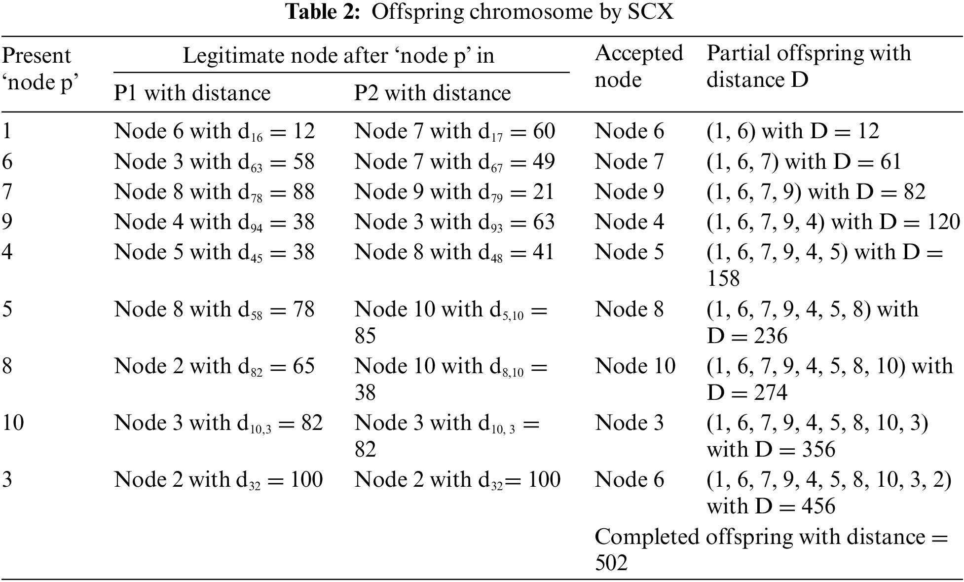
In [8], the SCX is suggested for the TSP that produces a good quality solution for both symmetric and asymmetric TSPLIB instances, which is compared with the other two crossover operators and found to be the best. It builds an offspring chromosome using better edges based on the edge values appearing in the parent chromosome. It also uses good-quality edges which are not present in either parent. It searches sequentially both parents and accepts the first unvisited node that is found after the present node. If an unvisited node is not seen in both parents, it searches sequentially from the start of the chromosome and picks the first unvisited node. A comparative study is reported in [32], which reports that SCX is the best among eight crossovers. The algorithm for the SCX [8] is presented in Algorithm 1.

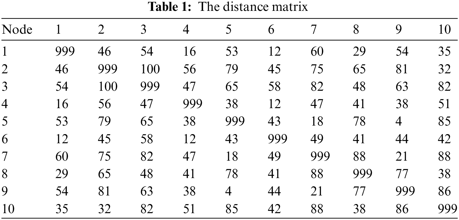
We consider the 10-node problem given as a distance matrix in Table 1. Let P1: (1, 6, 3, 9, 4, 5, 7, 8, 2, 10) and P2: (1, 7, 9, 3, 2, 4, 8, 5, 10, 6) be a pair of chosen parent chromosomes with distances 447 and 558 respectively. We use these chromosomes for applying to all crossover operators. We set the headquarters (first gene) as ‘node 1’, and so, the procedures are started from the ‘node 1’. Applying the SCX on the parent chromosomes, one can obtain the offspring O: (1, 6, 7, 9, 4, 5, 8, 10, 3, 2) with the distance 502 (see Table 2).

3.2 Adaptive Sequential Constructive Crossover Operator

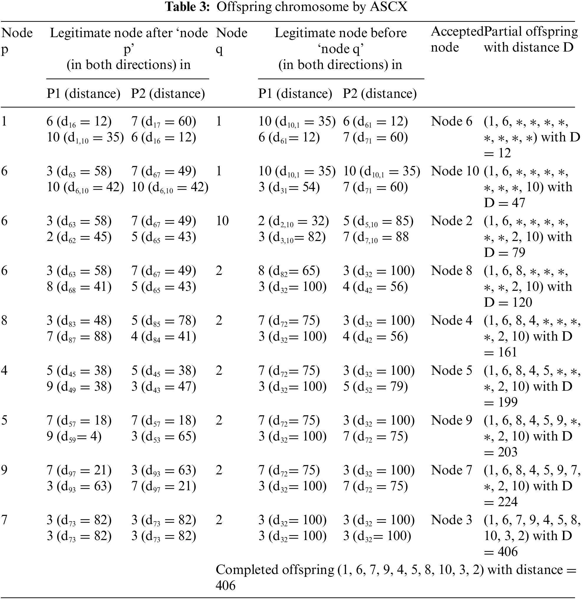
An adaptive SCX (ASCX) is developed in [33], which produces an offspring chromosome adaptively by searching in the forward/backward/mixed direction depending on distances to the next nodes. A comparative study amongst eight separate crossover operators shows that the operator ASCX is the best one. Algorithm 2 shows the pseudocode of the ASCX operator for the TSP.

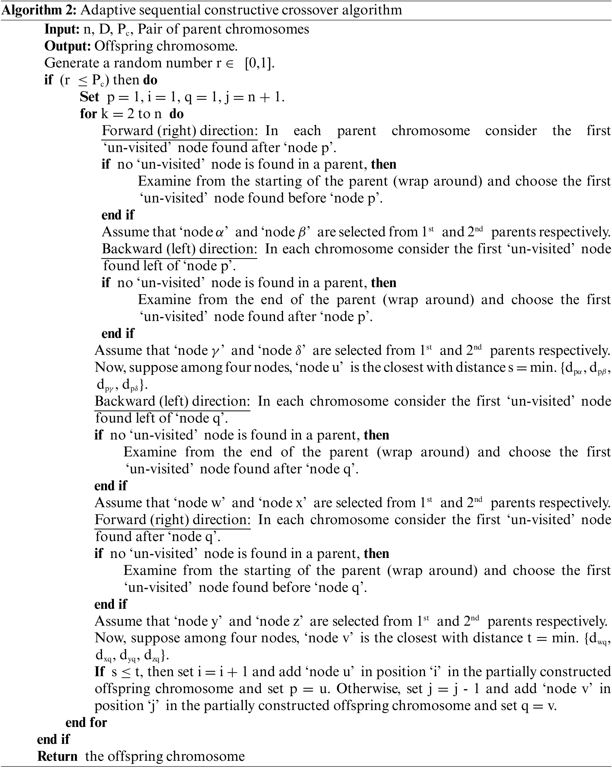
Applying the ASCX on the parent chromosomes, one can obtain the offspring O: (1, 6, 7, 9, 4, 5, 8, 10, 3, 2) with the distance 406 (see Table 3).

3.3 Greedy Sequential Constructive Crossover Operator

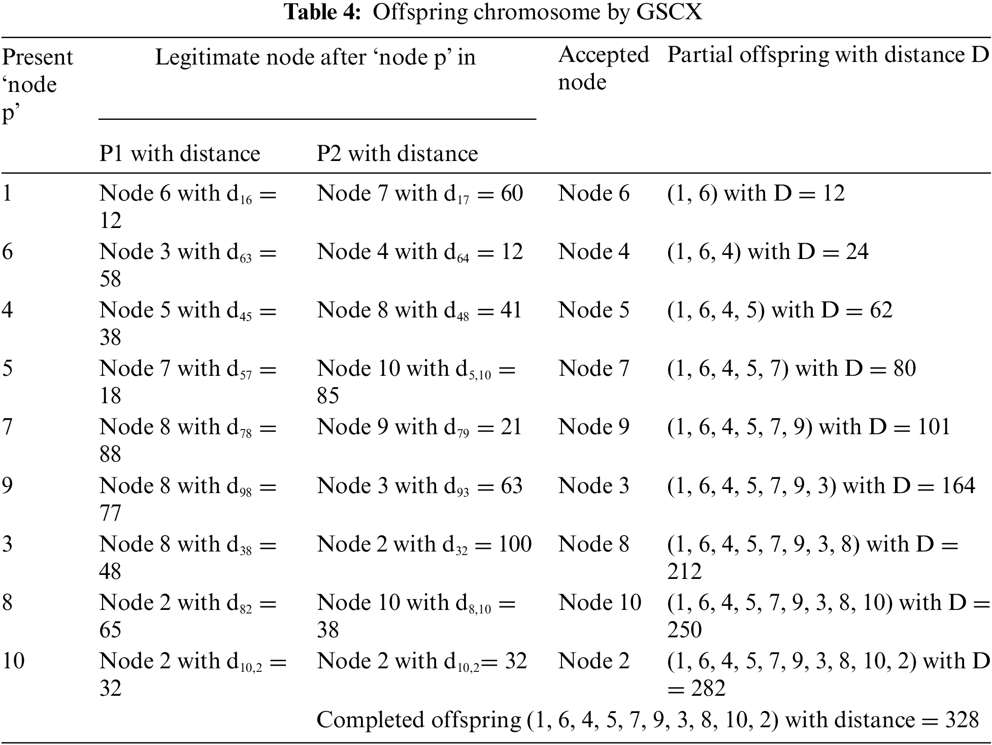
Furthermore, Ahmed [34] proposed another crossover named greedy SCX (GSCX) that produces an offspring chromosome using the greedy method adaptively by searching in the forward direction. Comparative studies among five different crossover operators show that the GSCX is the best one. Algorithm 3 shows the pseudocode of the GSCX operator for the TSP.

Applying the GSCX on the parent chromosomes, one can obtain the offspring O: (1, 6, 4, 5, 7, 9, 3, 8, 10, 2) with the distance 328 (see Table 4).

3.4 Reverse Greedy Sequential Constructive Crossover Operator

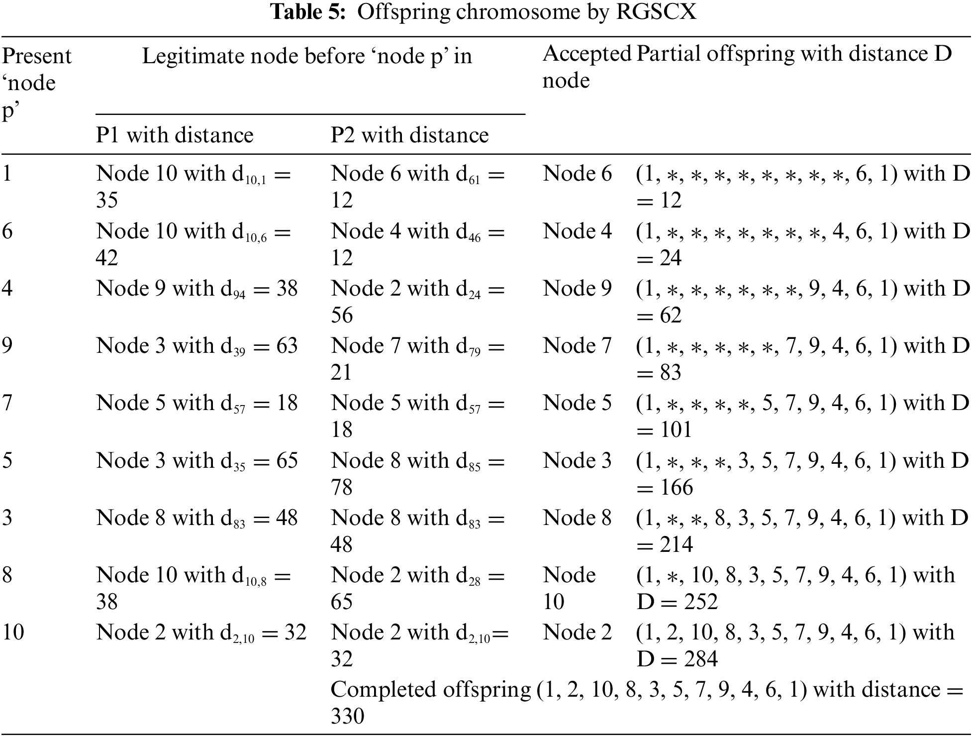
Ahmed [14] proposed another crossover named reverse greedy SCX (RGSCX) by applying the GSCX in the reverse direction that produces an offspring in the reverse direction, that is, from the last node (gene) of the offspring back to the first node (gene) of the same. Algorithm 4 shows the pseudocode of the RGSCX operator for the TSP.

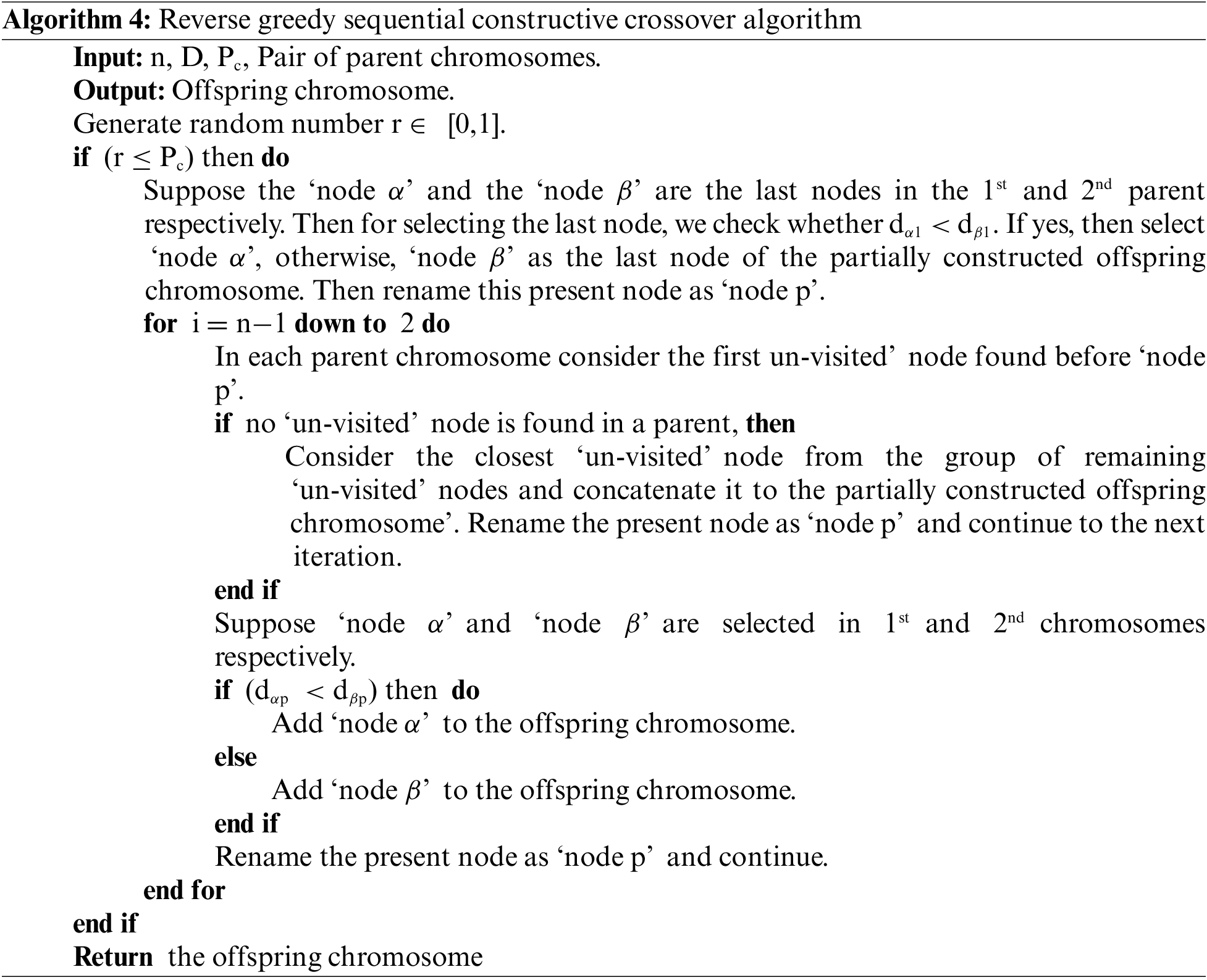
Applying the RGSCX on the parent chromosomes, one can obtain the offspring O: (1, 2, 10, 8, 3, 5, 7, 9, 4, 6, 1) with the distance 330 (see Table 5).

3.5 Comprehensive Sequential Constructive Crossover Operators

Ahmed [14] proposed a comprehensive SCX (CSCX) by combining GSCX and RGSCX that produces two offspring. Comparative studies among six different crossover operators show that the CSCX is the best one. We have considered a total of three comprehensive SCX operators for our study.

3.5.1 CSCX1

For a pair of parent chromosomes, the first offspring is generated using SCX and the second using RGSCX. Applying the CSCX1 to the parent chromosomes, one can obtain the following offspring:

O1: (1, 6, 7, 9, 4, 5, 8, 10, 3, 2) with the distance 502.

O2: (1, 2, 10, 8, 3, 5, 7, 9, 4, 6) with the distance 330.

3.5.2 CSCX2

For a pair of parent chromosomes, the first offspring is generated using GSCX and the second using RGSCX. Applying the CSCX2 to the parent chromosomes, one can obtain the following offspring:

O1: (1, 6, 4, 5, 7, 9, 3, 8, 10, 2) with the distance 328

O2: (1, 2, 10, 8, 3, 5, 7, 9, 4, 6) with the distance 330.

3.5.3 CSCX3

For a pair of parent chromosomes, the first offspring is generated using ASCX and the second using RGSCX. Applying the CSCX3 to the parent chromosomes, one can obtain the following offspring:

O1: (1, 6, 7, 9, 4, 5, 8, 10, 3, 2) with the distance 406.

O2: (1, 2, 10, 8, 3, 5, 7, 9, 4, 6) with the distance 330.

4  Mutation Operators for Our GAs

In GAs, diversity in the population is increased by introducing random variation in the population which is done in the mutation process. In this process, a gene in a chromosome is selected randomly and the corresponding gene is changed, thus, the information is modified. The following six mutation operators are used for our comparative study. Each operator is applied under the mutation probability, Pm, rule. We discuss all mutation operators through the chromosome P: (1, 6, 7, 9, 4, 5, 8, 10, 3, 2).

4.1 Exchange Mutation

In the exchange mutation (EXCH) process, two positions are selected randomly, and then the genes on these positions are exchanged [25]. For example, if positions 3 and 7 are selected randomly, genes 7 and 10 are exchanged with their positions, then the mutated chromosome will be O: (1, 6, 10, 9, 4, 5, 8, 7, 3, 2).

4.2 3-Exchange Mutation

In the 3-exchange mutation (3-EXCH) process, three different positions are randomly selected, say, r1, r2, and r3, then the genes on these positions are exchanged as follows: P(r1) ↔ P(r2) and then P(r2) ↔ P(r3) [35]. For example, if positions 2, 6, and 9 are randomly selected, then genes 6 and 5 are exchanged that leads to the chromosome (1, 5, 7, 9, 4, 6, 8, 10, 3, 2), and then genes 6 and 3 are exchanged that leads to the mutated chromosome as O: (1, 5, 7, 9, 4, 3, 8, 10, 6, 2).

4.3 Displacement Mutation

In the displacement mutation (DISP) process, a subchromosome is selected randomly and inserted at any random position outside the subchromosome [27]. For example, if the subchromosome (6, 7, 9, 4, 5) is selected randomly and the position between 8 and 9 is selected randomly for insertion, then the mutated chromosome will be O: (1, 8, 10, 6, 7, 9, 4, 5, 3, 2).

4.4 Insertion Mutation

In the insertion mutation (INST) process, a gene is chosen randomly and is inserted at any random location in the chromosome [15]. For example, if gene 3 is selected randomly and the position between 4 and 5 is selected randomly, then the mutated chromosome will be O: (1, 6, 7, 9, 3, 4, 5, 8, 10, 2).

4.5 Inversion Mutation

In the inversion mutation (INVS) process, two positions are selected randomly, and the genes between these positions are inverted [26]. For example, if two positions 4 and 8 are selected randomly, then the subchromosome (9, 4, 5, 8, 10) is inverted leading to the mutated chromosome as O: (1, 6, 7, 10, 8, 5, 4, 9, 3, 2).

4.6 Adaptive Mutation

In the adaptive mutation (ADAP) process, data from all chromosomes of the current population are gathered to detect a pattern among them. If the mutation is to be performed, chromosomes that do not like the pattern will be muted. The algorithm is as follows [30]:

Step 1: Consider all chromosomes in the current population.

Step 2: Construct a one-dimensional array of size n (size of the problem), suppose A, by storing a gene that appears the minimum number of times in the current position (except the 1st position) of all chromosomes.

Step 3: If the mutation is allowed, select two genes randomly such that they are not the same in the corresponding positions of array A, and swap them.

For example, suppose A = [1, 5, 2, 3, 6, 2, 5, 7, 10, 8] is the array and 4th and 8th positions are selected randomly. The 4th position’s gene 9 and the 8th position’s gene 10 do not match the array elements in the corresponding positions, so they are exchanged. So, the mutated chromosome will be O: (1, 6, 7, 10, 4, 5, 8, 9, 3, 2).

Our GA is a simple, non-hybrid that uses traditional GA operators and processes. In our GA, initiating with a random chromosome population, the better chromosomes are chosen by the stochastic remainder selection method, and then the population passes through the selected one crossover operator and one mutation operator. Our simple GA may be designed as follows:

SimpleGA()

{ Initialize a random population of size Ps.

    Evaluate the population.

    Generation = 0.

    While the stopping condition is not satisfied

    { Generation = Generation + 1.

       Select fitter chromosomes by selection operator.

       Select a crossover operator and do a crossover with crossover probability Pc.

       Select a mutation operator and do a mutation with mutation probability Pm.

       Evaluate the population.

    }

}

5  Computational Experiments

We have encoded different simple GAs using various crossover and mutation processes in Visual C++ and executed some TSPLIB instances [13] on a Laptop with Intel(R) Core(TM) i7-1065G7 CPU @ 1.30 GHz and 8.00 GB RAM under MS Windows 11. For each instance, the experiments have been done 50 times. We measured the solution quality by the percentage of excess (EX(%)) of the obtained best solution (OBS) from the best-known solution (BKS) informed on the TSPLIB website, using the formula: EX (%) = 100 × (OBS/BKS-1). We report the best solution (BS), average solution (AS), percentage of excess of the best solution (BEX(%)), and percentage of excess of average solution (AEX(%)) over the BKS among 50 executions, standard deviation (SD) of the solutions in 50 executions, average computational time (AT) (in seconds) to find the best solution for the first time for each instance using each algorithm. To avoid preference for any distinct algorithm, the same randomly generated population is used for executing the proposed algorithms. Notice that GAs are controlled by parameters-population size (Ps), crossover probability (Pc), mutation probability (Pm), and termination condition.

We set Ps = 50, Pc = 1.0 (i.e., 100%) as the crossover probability to see the real behavior of the crossover operators and almost the same computational time as a termination criterion. First, we see the functioning of the crossover operators on fourteen asymmetric TSPLIB instances. Table 6 shows the comparative study amongst GAs using seven crossover operators without using any mutation operator. In this table, the first column reports an instance name and its BKS within brackets. The second column reports the data names and the remaining columns report the corresponding results by different crossover operators mentioned in the first row. Furthermore, the boldfaces in the results indicate that the result by a particular algorithm is the best one amongst all algorithms for a particular instance.

Looking at the boldfaces in Table 6, the comprehensive crossover operators are observed better than the other crossover operators. Operator CSCX1 could find the best solution for ten instances–ftv33, ftv35, p43, ftv44, ftv47, ry48p, ft53, ftv64, ftv70 and kro124p, whereas CSCX2 could find for six instances–ftv35, ftv38, ftv44, ftv55, ft70 and ftv170. Furthermore, CSCX1 could find the best average solution for two instances–ry48p and ft53; whereas CSCX2 could find for ten instances–ftv35, ftv38, ftv44, ftv47, ftv55, ftv64, ft70, ftv70, kro124p and ftv170; and CSCX3 for two instances–ftv33 and p43. It is seen that two operators–CSCX1 and CSCX2 are competing. However, CSCX2 is observed better than CSCX1, and CSCX1 is found to be better than CSCX3. So, CSCX2 is the best crossover operator among all crossover operators without using any mutation operator. Among other crossover operators, ASCX, GSCX, and RGSCX could find the best solutions for three, six, and five instances, respectively. Further, ASCX, GSCX, and GSCX could find the best average solution for twelve, two, and zero instances, respectively. Two operators–ASCX and GSCX are competing. However, looking at the average solutions and standard deviations, we can conclude that ASCX is better than GSCX. Looking at the average computational times by the GAs using these crossover operators, almost all algorithms are taking almost the same time.

Accordingly, CSCX2 produces the best results, while CSCX1 is the second best, ASCX and CSCX3 are competing for the third best, and SCX is the worst one. However, it is confirmed that ASCX, GSCX, and RSCX are the improvements of SCX. The results are also depicted in Fig. 1, which also demonstrates the usefulness of CSCX2 and CSCX1. Further, Fig. 1 shows that for most of the instances, SCX finds the worst solution quality, and other algorithms find improved solutions over the solutions by SCX. The operators ASCX and CSCX3 are competing for the third position.

Figure 1: Average Excess (%) by different crossovers for asymmetric instances

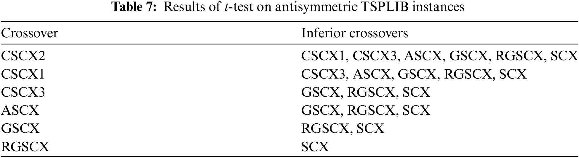
Furthermore, to justify the above observations, the two-tailed Student t-test was conducted with a 5% significant level between CSCX2 and other crossover operators for the instances, and the results are summarized in Table 7. As expected, CSCX2 is the best-ranked crossover and CSCX1 is the second-best. Between CSCX3 and ASCX, there is no significant difference, as expected, they are in the third rank.

We now implement different mutation operators with the probability of mutation as 0.10 (10%) without any crossover operator on the same TSPLIB instances. Table 8 shows the comparative study among GAs using six mutation operators without any crossover operator.

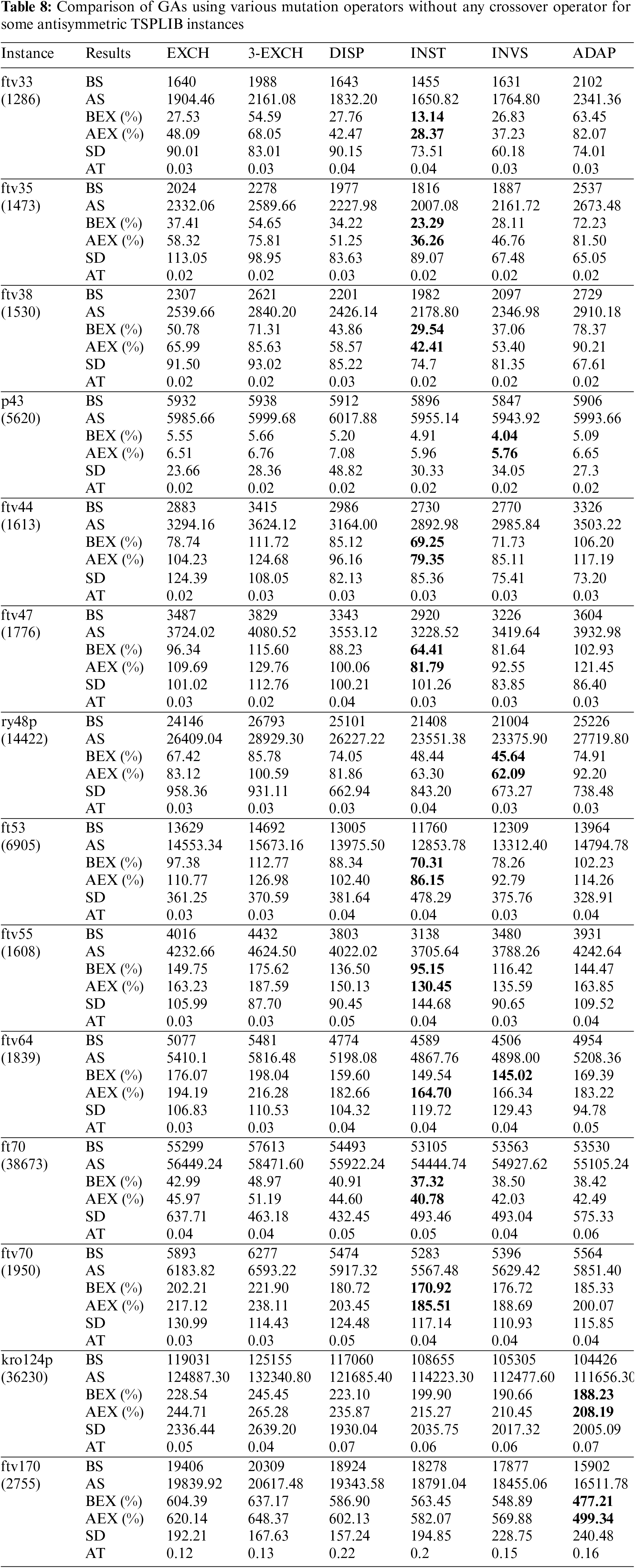
Looking at the boldfaces in Table 8, the mutation operators EXCH, 3-EXCH, and DISP could not find the best solution for any instance. The mutation operator could find the best solution for nine instances–ftv33, ftv35, ftv38, ftv44, ftv47, ft53, ftv55, ft70, and ftv70; whereas INVS could find it for three instances–p43, ry48p, and ftv64; and ADAP could find for two instances kro124p and ftv170. Furthermore, EXCH, 3-EXCH, and DISP could not find the best average solution for any instance, whereas INST could find for ten instances–ftv33, ftv35, ftv38, ftv44, ftv47, ft53, ftv55, ftv64, ft70, and ftv70; INVS could find for two instances–p43 and ry48p; and ADAP could find for two instances–kro124p and ftv170. It is clear that the INST is the best one, and the two operators–INVS and ADAP are competing for the second best. The operators EXCH, 3-EXCH, and DISP could neither find the best solution nor find the best average solution for any instance, hence, they are not good enough for the TSP in comparison to the other three operators. Looking at the average computational times by the GAs using these mutation operators, almost all algorithms are taking almost the same time.

The results are also depicted in Fig. 2, which also demonstrates the usefulness of INST, INVS, DISP, and ADAP mutation operators. It is very clear from the figure that INST mutation is the best and INVS is the second best for the problem instances of size less than 100, and ADAP is the best, and INVS and INST are competing for the second best, for the problem instances of size more than or equal to 100.

Figure 2: Average Excess (%) by different mutations for asymmetric instances

So, we have conducted the two-tailed Student t-test with a 5% significant level between INST and other mutation operators for the instances. However, the results are not reported here. As expected, INST is the best-ranked mutation and INVS is the second best. However, DISP is placed in third place and ADAP is placed in fourth place.

We now implement different mutation operators with the crossover operators using the common mutation probability. However, it is not easy to fix mutation probability for all mutation operators for all instances. After doing extensive experiments, we fix Pm = 0.10 and a maximum of 2000 generations for the termination condition. Table 9 shows the comparative study among simple GAs using all seven crossover operators without any mutation operator and with six mutation operators on fourteen asymmetric TSPLIB instances. In the first column, we report the instance name, and its best-known solution value within the brackets informed on the TSPLIB website. The second column reports the name of the mutation operator, the second last column reports the grand average of the average excess (%) (GAVG) using a particular mutation operator and all crossover operators, and the last column reports the average percentage of improvement (IMPV) by GAs using a particular mutation operator over GAs without any mutation operator. The remaining columns report the average excess (%) by a crossover operator without using any mutation and using all six mutation operators as mentioned therein.

By looking at the partial average of average excess (%) (PAVG) (in boldface), regardless of any mutation operator, in Table 9, operators SCX, ASCX, GSCX, RGSCX, and CSCX3 could not find best average for any instance, CSCX1 is found to be the best for five instances, namely, p43, ftv47, ft53, ft70 and ftv70; CSCX2 is found to be best for nine instances–ftv33, ftv35, ftv38, ftv44, ry48p, ftv55, ftv64, kro124p and ftv170. Hence, CSCX2 is observed as the best one, CSCX1 is the second best, CSCX3 is the third best, and ASCX is the fourth best. CSCX1 and CSCX2 are competing and are very close to each other. Looking at the last column, IMPV, it is confirmed that using the mutation operator in GA has a great impact on the solution quality of the problem instances. The PAVG that is shown in Table 9 is also depicted in Fig. 3. Looking at the figure, it is very clear that SCX with mutation operators is the worst one and all other crossover operators with mutation operators have some improvement over the SCX with mutation operators. Though CSCX1 and CSCX2 both with mutations are competing with each other, however, CSCX2 with mutations is the best one, CSCX1 with the mutations is the second best, and CSCX3 with mutations is the third best.

Figure 3: Comparative study of seven different crossover operators

By looking at the grand average of the average excess (%) (GAVG) (in boldface), regardless of any crossover operator, in Table 9, EXCH is found to be the best for only one instance–ftv47; 3-EXCH is the best for five instances–p43, ftv44, ft53, ftv64, and kro124p; DISP is best for only one instance–ft70; INST is best for three instances–ftv33, ftv35 and ftv64; INVS is found best for one instance–ry48p; and ADAP is best for three instances–ftv38, ftv55 and ftv170. Hence, it is observed that 3-EXCH is the best one, then INST and ADAP are the second best, and then EXCH, DISP, and INVS are the third best. Further, looking at the last column, which shows the average improvement using crossover operators with different mutation operators over GAs using only crossover operators without using any mutation, it confirmed our observation. It is noted that all GAs using mutation have significant improvements over GAs without any mutation operator. The GAVG that is shown in Table 9 is also depicted in Fig. 4, which further confirms our observation, and shows clear improvement of GAs with crossover and mutation operators over GAs with crossover operators and without any mutation operator.

Figure 4: Comparative study of different mutation operators

Since CSCX2 with mutation operators is the best one and CSCX1 with mutation operators is the second best, we now look at the combinations of CSCX1 with any mutation and CSCX2 with any mutation, in Table 9. We mark by superscripta for the best average excess (%) using CSCX1 with any mutation operator for instance, and we mark by superscriptb for the best average excess (%) using CSCX2 with any mutation operator for instance.

By looking at the average excess (%) (marked by superscripta), in Table 9, the combination of CSCX1 and EXCH is found to be best for only one instance–p43; the combination of CSCX1 and 3-EXCH is best for only one instance–p43; the combination of CSCX1 and DISP is best for three instances–ry48p, ft70 and kro124p; combination of CSCX1 and INST is found to be best for four instances–ftv33, ftv35, ftv47 and ft53; combination of CSCX1 and INVS is best for only one instance-ftv44; combination of CSCX1 and ADAP is best for five instances–ftv38, ftv55, ftv64, ftv70 and ftv170. Hence, the combination of CSCX1 and ADAP is the best one, and the combination of CSCX1 and INST is the second best, and the combination of CSCX1 and DISP is the third best.

By looking at the average excess (%) (marked by superscriptb), in Table 9, the combination of CSCX2 and EXCH is found to be best for two instances–ftv47 and ftv55; the combination of CSCX2 and 3-EXCH is best for only one instance–ftv44; the combination of CSCX2 and DISP is best for five instances–ft53, ftv64, ft70, ftv70, and kro124p; the combination of CSCX2 and INST is found to be best for two instances–ftv33 and ftv38; the combination of CSCX2 and INVS is best for three instances–ftv35, p43, and ry48p; the combination of CSCX2 and ADAP is best for only one instance-ftv170. Hence, the combination of CSCX2 and DISP is the best one, the combination of CSCX2 and INVS is the second best, and the combination of CSCX2 and INST, and CSCX2 and EXCH are the third best.

Finally, regardless of the combination of any crossover and any mutation operator, by looking at the average excess (%) (marked by boldface superscripta or superscriptb), in Table 9, the combination of CSCX1 and EXCH, and, the combination of CSCX1 and 3-EXCH is found to be best for only one instance–p43; the combination of CSCX1 and DISP is found to be best for two instances–ft70 and kro124p; the combination of CSCX1 and INST is found to be best for four instances–ftv33, ftv35, ftv47 and ft53. The remaining combinations of CSCX1 and ADAP, CSCX2 and EXCH, CSCX2 and 3-EXCH, CSCX2 and DISP, CSCX2 and INST, CSCX2 and INVS, CSCX2 and ADAP, are observed as the best for only one instance each. Hence, among all combinations, the combination of CSCX1 and INST is observed as the best one, and the combination of CSCX1 and DISP is the second best. Looking at Table 9, one can see that GA using CSCX1 and INST could find average solutions whose average percentage of excesses from the best-known solutions are 5.61, 2.43, 4.57, 0.22, 3.87, 4.30, 6.04, 9.65, 3.79, 2.80, 5.90, 2.21, 9.67 and 14.94 for ftv33, ftv35, ftv38, p43, ftv44, ftv47, ry48p, ft53, ftv55, ftv64, ft70, ftv70, kro124p and ftv170, respectively.

6  Conclusions and Future Work

Simple genetic algorithms using seven crossover operators and six mutation operators are suggested for the well-known travelling salesman problem (TSP). First, the crossover and mutation operators were illustrated through some example chromosomes. Then, experimental studies have been carried out on the benchmark TSPLIB instances. To observe the real behavior of different crossover operators, we implemented simple genetic algorithms using seven different crossover operators with a cent percentage of crossover probability and without any mutation operator on the benchmark instances. It can be seen from our study that comprehensive sequential constructive crossovers are very effective, especially, since CSCX2 is the best one and CSCX1 is the second best. Next, to observe the behavior of different mutation operators, we implemented simple genetic algorithms using six different mutation operators with ten percentage of mutation probability and without any crossover operator on the benchmark instances. It can be seen from our study that insertion mutation is the best one, inversion mutation is the second best, and displacement mutation is the third best. To observe the behavior of the combination of different mutation and crossover operators, we implemented simple genetic algorithms using seven crossover and six different mutation operators on the benchmark instances. By looking at the percentage of average solution excess, one can see from our study that the combination of CSCX-1 and insertion mutation is observed as the best one, and the combination of CSCX-1 and displacement mutation is the second best. The GA using CSCX1 with insertion mutation could find average solutions whose average percentage of excesses from the best-known solutions are between 0.22 and 14.94 for our experimented problem instances.

Our aim in this study was only to compare several crossover operators and several mutation operators regarding the solution quality. Our aim was not to improve the solution quality, so, we did not incorporate any local search method to enhance the solution quality. Although the combination of comprehensive sequential constructive crossover and insertion mutation was observed as the best, it still could not obtain the exact solution to many experimented problem instances. Of course, a thoroughly fine-tuned parameter set, that is, crossover probability, population size, mutation probability, etc., may find better quality solutions. Some literature combines metaheuristic and exact algorithms, and uses sub-tour division [36], to find better solutions. We also plan to combine an exact method and a metaheuristic algorithm to find better-quality solutions to the problem instances.

Acknowledgement: The authors are very much thankful to the anonymous honorable reviewers for their careful reading of the paper and their many insightful comments and constructive suggestions which helped the authors to improve the paper. The authors further are very much thankful to the Deanship of Scientific Research at Imam Mohammad Ibn Saud Islamic University (IMSIU) for its financial support.

Funding Statement: This work was supported and funded by the Deanship of Scientific Research at Imam Mohammad Ibn Saud Islamic University (IMSIU) (Grant Number IMSIU-RP23030).

Author Contributions: The authors confirm their contribution to the paper as follows: study conception and design: Z. H. Ahmed; data collection and implementation: H. Haron, A. Al-Tameem; analysis and interpretation of results: Z. Ahmed, H. Haron, A. Al-Tameem; draft manuscript preparation: H. Haron; final manuscript preparation and revision: Z. H. Ahmed, A. Al-Tameem. All authors reviewed the results and approved the final version of the manuscript.

Availability of Data and Materials: The data that support the findings of this study are openly available in the TSPLIB repository at http://www.iwr.uni-heidelberg.de/groups/comopt/software/TSPLIB95/tsp.

Conflicts of Interest: The authors declare that they have no conflicts of interest to report regarding the present study.

References

1. R. M. Karp, Reducibility among Combinatorial Problems. Boston, MA: Springer, 1972, pp. 85–103. [Google Scholar]

2. A. Larni-Fooeik, N. Ghasemi, and E. Mohammadi, “Insights into the application of the traveling salesman problem to logistics without considering financial risk: A bibliometric study,” Manage. Sci. Lett., vol. 14, no. 3, pp. 189–200, 2024. doi: 10.5267/j.msl.2023.11.002. [Google Scholar] [CrossRef]

3. W. Zhang, J. J. Sauppe, and S. H. Jacobson, “Results for the close-enough traveling salesman problem with a branch-and-bound algorithm,” Comput. Optim. Appl., vol. 85, no. 2, pp. 369–407, 2023. doi: 10.1007/s10589-023-00474-3. [Google Scholar] [CrossRef]

4. T. Q. T. Vo, M. Baiou, and V. H. Nguyen, “A branch-and-cut algorithm for the balanced traveling salesman problem,” J. Comb. Optim., vol. 47, no. 4, pp. 515, 2024. doi: 10.1007/s10878-023-01097-4. [Google Scholar] [CrossRef]

5. R. Carr, R. Ravi, and N. Simonetti, “A new integer programming formulation of the graphical traveling salesman problem,” Math. Program., vol. 197, no. 2, pp. 877–902, 2023. doi: 10.1007/s10107-022-01849-w. [Google Scholar] [CrossRef]

6. Z. H. Ahmed and I. Al-Dayel, “An exact algorithm for the single-depot multiple travelling salesman problem,” IJCSNS Int. J. Comput. Sci. Netw. Secur., vol. 20, no. 9, pp. 65–75, 2020. [Google Scholar]

7. Y. Wang and Z. Han, “Ant colony optimization for traveling salesman problem based on parameters optimization,” Appl. Soft Comput., vol. 107, no. 2, pp. 107439, 2021. doi: 10.1016/j.asoc.2021.107439. [Google Scholar] [CrossRef]

8. Z. H. Ahmed, “Genetic algorithm for the traveling salesman problem using sequential constructive crossover operator,” Int. J. Biomet. Bioinform., vol. 3, no. 6, pp. 96–105, 2010. [Google Scholar]

9. İ. İlhan and G. Gökmen, “A list-based simulated annealing algorithm with crossover operator for the traveling salesman problem,” Neural Comput. Appl., vol. 34, no. 10, pp. 7627–7652, 2022. doi: 10.1007/s00521-021-06883-x. [Google Scholar] [CrossRef]

10. M. Gendreau, G. Laporte, and F. Semet, “A tabu search heuristic for the undirected selective travelling salesman problem,” Eur. J. Oper. Res., vol. 106, no. 2–3, pp. 539–545, 1998. doi: 10.1016/S0377-2217(97)00289-0. [Google Scholar] [CrossRef]

11. Y. Cui, J. Zhong, F. Yang, S. Li, and P. Li, “Multi-subdomain grouping-based particle swarm optimization for the traveling salesman problem,” IEEE Access, vol. 8, pp. 227497–227510, 2020. doi: 10.1109/ACCESS.2020.3045765. [Google Scholar] [CrossRef]

12. D. E. Goldberg, Genetic Algorithms in Search, Optimization, and Machine Learning. New York: Addison-Wesley, 1989. [Google Scholar]

13. G. Reinelt, “TSPLIB—A traveling salesman problem library,” ORSA J. Comput., vol. 3, no. 4, pp. 376–384, 1991. Accessed: Nov. 20, 2023. [Online]. Available: http://comopt.ifi.uni-heidelberg.de/software/TSPLIB95/ [Google Scholar]

14. Z. H. Ahmed, “Genetic algorithm with comprehensive sequential constructive crossover for the travelling salesman problem,” Int. J. Adv. Comput. Sci. Appl., vol. 11, no. 5, pp. 245–254, 2020. doi: 10.14569/IJACSA.2020.0110533. [Google Scholar] [CrossRef]

15. D. B. Fogel, “An evolutionary approach to the travelling salesman problem,” Biol. Cybern., vol. 60, no. 2, pp. 139–144, 1988. doi: 10.1007/BF00202901. [Google Scholar] [CrossRef]

16. J. J. Grefenstette, “Incorporating problem specific knowledge into genetic algorithms,” in L. Davis (Ed.Genetic Algorithms and Simulated Annealing, London, UK: Pitman/Pearson, 1987, pp. 42–60. [Google Scholar]

17. L. Davis, “Job-shop scheduling with genetic algorithms,” in Proc. Int. Conf. Genetic Algor. Appl., 1985, pp. 136–140. [Google Scholar]

18. B. Freisleben and P. Merz, “A genetic local search algorithm for solving symmetric and asymmetric traveling salesman problems,” in Proc. 1996 IEEE Int. Conf. Evol. Comput., Nagoya, Japan, 1996, pp. 616–621. [Google Scholar]

19. D. E. Goldberg and R. Lingle, “Alleles, loci and the travelling salesman problem,” in J. J. Grefenstette (Ed.Proc. First Int. Conf. Genetic Algor. Appl., Hilladale, NJ, Lawrence Erlbaum Associates, 1985. [Google Scholar]

20. G. Syswerda, “Schedule optimization using genetic algorithms,” in L. Davis (Ed.Handbook of Genetic Algorithms, New York: Van Nostrand Reinhold, 1991, pp. 332–349. [Google Scholar]

21. I. M. Oliver, D. J. Smith, and J. R. C. Holland, “A study of permutation crossover operators on the travelling salesman problem,” in J. J. Grefenstette (Ed.Proc. First Int. Conf. Genetic Algor. Appl., Hilladale, NJ, Lawrence Erlbaum Associates, 1987. [Google Scholar]

22. J. Grefenstette, R. Gopal, B. Rosmaita, and D. Gucht, “Genetic algorithms for the traveling salesman problem,” in J. J. Grefenstette (Ed.Proc. First Int. Conf. Genetic Algor. Appl., Mahwah, NJ, Lawrence Erlbaum Associates, 1985, pp. 160–168. [Google Scholar]

23. N. J. Radcliffe and P. D. Surry, “Formae and variance of fitness,” in D. Whitley, M. Vose (Eds.Foundations of Genetic Algorithms 3, San Mateo, CA: Morgan Kaufmann, 1995, pp. 51–72. [Google Scholar]

24. D. Whitley, T. Starkweather, and D. Shaner, “The traveling salesman and sequence scheduling: Quality solutions using genetic edge recombination,” in L. Davis (Ed.Handbook of Genetic Algorithms. New York: Van Nostrand Reinhold, 1991, pp. 350–372. [Google Scholar]

25. W. Banzhaf, “The molecular traveling salesman,” Biol. Cybern., vol. 64, no. 1, pp. 7–14, 1990. doi: 10.1007/BF00203625. [Google Scholar] [CrossRef]

26. D. Fogel, “A parallel processing approach to a multiple travelling salesman problem using evolutionary programming,” in Proc. Fourth Annual Symp. Parallel Process., Fullerton, California, 1990, pp. 318–326. [Google Scholar]

27. Z. Michalewicz, Genetic Algorithms + Data Structures = Evolution programs. Berlin: Springer-Verlag, 1992. [Google Scholar]

28. M. Gen and R. Cheng, Genetic Algorithm and Engineering Design. New York: John Wiley and Sons, 1997, pp. 118–127. [Google Scholar]

29. S. J. Louis and R. Tang, “Interactive genetic algorithms for the traveling salesman problem,” in Proc. Genetic Evol. Comput. Conf. (GECCO), 1999, pp. 385–392. [Google Scholar]

30. Z. H. Ahmed, “An improved genetic algorithm using adaptive mutation operator for the quadratic assignment problem,” in Proc. 37th Int. Conf. Telecommun. Signal Process (TSP 2014), Berlin, Germany, 2014, pp. 616–620. [Google Scholar]

31. A. B. Doumi, B. A. Mahafzah, and H. Hiary, “Solving traveling salesman problem using genetic algorithm based on efficient mutation operator,” J. Theor. Appl. Inf. Technol., vol. 99, no. 15, pp. 3768–3781, 2021. [Google Scholar]

32. I. H. Khan, “Assessing different crossover operators for travelling salesman problem,” IJISA Int. J. Intell. Syst. Appl., vol. 7, no. 11, pp. 19–25, 2015. doi: 10.5815/ijisa.2015.11.03. [Google Scholar] [CrossRef]

33. Z. H. Ahmed, “Adaptive sequential constructive crossover operator in a genetic algorithm for solving the traveling salesman problem,” IJACSA Int. J. Adv. Comput. Sci. Appl., vol. 11, no. 2, pp. 593–605, 2020. doi: 10.14569/issn.2156-5570. [Google Scholar] [CrossRef]

34. Z. H. Ahmed, “Solving the traveling salesman problem using greedy sequential constructive crossover in a genetic algorithm,” IJCSNS Int. J. Comput. Sci. Netw. Secur., vol. 20, no. 2, pp. 99–112, 2020. [Google Scholar]

35. Z. H. Ahmed, “Experimental analysis of crossover and mutation operators for the quadratic assignment problem,” Ann. Oper. Res., vol. 247, no. 2, pp. 833–851, 2016. doi: 10.1007/s10479-015-1848-y. [Google Scholar] [CrossRef]

36. R. Jain et al., “Application of proposed hybrid active genetic algorithm for optimization of traveling salesman problem,” Soft Comput., vol. 27, no. 8, pp. 4975–4985, 2023. doi: 10.1007/s00500-022-07581-z. [Google Scholar] [CrossRef]