Curve Classification Based on Mean-Variance Feature Weighting and Its Application

1  Introduction

Functional data analysis (FDA) [1] is an active research field for analyzing random curves or other multidimensional functional data. With the improvement of data collection technology, functional data is rapidly emerging in various fields. FDA techniques are also constantly evolving. There is a substantial overlap between time series data and functional data. Functional data generally contain smooth random functions, and the domain of functional data can be more than time. The random function inherent in functional data is usually characterized by a random process and analyzed through observed functional trajectories. Compared to multivariate data, functional data is infinite-dimensional. The high intrinsic dimensionality of these data brings challenges for theory as well as computation. Usually, the primary task of the FDA is dimensionality reduction.

Among many others, the classification of functional data, such as pattern recognition and medical diagnosis, is becoming increasingly important in research. Recently, Blanquero et al. [2] addressed the problem of selecting the most informative time instants in multivariate functional data. Jiang et al. [3] presented a supervised functional principal component analysis to extract image-based features associated with the failure time. Castro Guzman et al. [4] proposed a convolution-based linear discriminant analysis for functional data classification. Weishampel et al. [5] proposed a method that can classify a binary time series using nonparametric approaches. These researches aim to improve the classification accuracy of complex functional data, which could be helpful for practical application research in medicine, remote sensing, and other fields.

Generally, the classification approaches of functional data can mainly be divided into three types: Model-based, density-based, and algorithm-based methods. The model-based functional classification methods [6–8] tend to find relationships between functional predictors and class labels. The density-based functional classification methods [9–12] mainly use Bayes classifiers for functional data classification. The algorithm-based functional classification methods [13–15] prefer to project the functional data to a finite-dimensional space and then use machine learning or statistical learning methods for classification.

In the algorithm-based functional classification, most studies approximate each functional curve by a linear combination of a set of basis functions. Functional principal component analysis [16–18] is a powerful tool to extract the major modes of variation in the functional data. The first several functional principal components can characterize the information of functional data. Otherwise, prior basis function expansion is widely used for extracting low-dimensional features, such as B-spline basis [19–21] and Fourier basis [22]. Afterwards, some classical classification methods can be used for the extracted features, such as linear discriminant analysis (LDA) [13,14], K-nearest neighbor (KNN) [23], and support vector machine (SVM) [24], etc.

In order to minimize the loss of information in functional data, retaining more features during the feature extraction stage is usually necessary. However, these features often contain redundancies that affect classification accuracy. A common strategy to address this problem is feature selection or feature weighting. In multivariate data analysis, there are many methods for feature selection [25,26] and feature weighting [27,28], including mutual information [29–32], information gain [24], and regularized entropy [33]. Some classification methods based on either feature selection or feature weighting have been extended to functional data. For instance, Li et al. [13] identified significant features using F-statistic and LDA, then used SVM for classification. Chang [34] proposed the rotation forest method combined with the patch selection for functional data classification.

However, these classification methods do not fully consider between-class differences and within-class variations of local features of functional data. When the local features have large differences between classes and minor within-class variations, they correspond to local significant features for classification. Feature selection methods tend to remove all insignificant features and retain only significant features for classification. With many redundant features, these methods can achieve a good dimensionality reduction effect. However, each feature is not ranked according to its own importance. Furthermore, using feature selection methods will risk losing information in some cases. For example, when handling data with small between-class differences and large within-class variations, the classification tasks become difficult. At this point, the feature weighting method is a better alternative, which tends to retain information and give more weight to significant features and less weight to insignificant features.

In this paper, we propose a new mean-variance-based feature weighting method constructed on the coefficient values. We adopt the B-spline approximation approach for extracting the coefficient features of functional data. From an intuitive perspective on classification, we directly let the ratio of between-class differences to within-class variations determine the weights of features. The size of each weight represents the individual contribution of each feature to classification. The quantified MV feature weights can strengthen significant features and compress redundant features. To summarize, the critical contributions of our proposal are briefly demonstrated as follows:

(1) An innovative feature weighting method based on statistical principles is introduced. Significant features become more dispersed, and insignificant features become more compact. It can effectively enhance the contribution of significant features and weaken the influence of confusing features for classification.

(2) The MV feature weighting method can also be integrated with classical functional classification methods. We can perform feature weighting on the extracted features or reconstructed functional data for classification. For instance, we integrate our method with the generalized functional linear model and functional linear discriminant analysis and achieve a significant improvement in classification.

The rest of this paper is structured as follows. Section 2 introduces the proposed MV feature weighting method. Section 3 evaluates the classification performance of our proposal through simulation studies. Section 4 presents the applications of some real data sets, followed by a conclusion in Section 5.

2  Methodology

Let {yi(t),i=1,…,n} be the observed functional data set, which can be modeled by

yi(t)=Φ(t)βi+ϵi,(1)

where Φ⊤(t)=(ϕ1(t),…,ϕp(t))⊤ are the basis functions, βi are the coefficients of the basis functions, and ϵi is the random error.

Suppose that the i-th discrete observations yi=(yi(ti1),…,yi(timi))⊤ are recorded at a series of time points ti=(ti1,…,timi)⊤, thus the model can be expressed in a matrix form:

yi=Φiβi+ϵi,(2)

where Φi⊤=(ϕ1(ti),…,ϕp(ti))⊤ is the p×mi dimensional basis matrix.

Because each sample curve can be approximated by the basis functions, the raw data can be represented by low-dimensional coefficient features. A widely used basis function is the B-splines. In the next section, we will demonstrate how to extract features with the B-splines.

2.1 Feature Extraction

A simple linear smoother is obtained if we estimate the coefficient vector by minimizing the objective function

J(βi)=(yi−Φiβi)⊤(yi−Φiβi),(3)

solving this for βi provides the ordinary least squares solution: β^i=(Φi⊤Φi)−1Φi⊤yi. In order to control of the smoothness of functional data, we add a second order difference roughness penalty to Eq. (3) to obtain the regularized objective function

RJ(βi)=(yi−Φiβi)⊤(yi−Φiβi)+λ‖Dβi‖2.(4)

Thus, the smooth estimate can be written by

β^i=(Φi⊤Φi+λD⊤D)−1Φi⊤yi,(5)

where D is the second order difference penalty matrix and λ is a smoothing parameter. The parameter selection strategy can be seen in [35,36].

By conducting the above estimation process, we can obtain the coefficient features of all sample curves. Next, we will introduce the calculation of feature weights.

2.2 The Estimation of Feature Weights

The mean and variance are elementary and important statistics to describe the data characteristics and we prefer to retain all features to make full use of all information. In binary classification, the between-class difference can be measured by the difference between two classes’ means, and the within-class variations can be measured by the sum of two classes’ variances. Thus, the MV weight can be calculated by

wj=|β¯j(1)−β¯j(2)|∑k=12∑i∈𝒞k(βij−β¯j(k))2,(6)

where 𝒞k is the indices of the nk samples in the k-th class, βij is the value of the i-th sample at the j-th feature, β¯j(k)=∑i∈𝒞kβij/nk is the mean of all samples of the k-th class at the j-th feature. In multi-class classification, the MV weight can be calculated by

wj=∑k=1K|β¯j(k)−β¯j|∑k=1K∑i∈𝒞k(βij−β¯j(k))2,(7)

where K is the number of classes and β¯j=∑i∈nβij/n is the mean of all samples at the j-th feature.

Then we can obtain original MV weight vector WMV=(W1,…,Wp)⊤ by normalizing, which satisfies Wj=wj/∑j=1pwj. For local features with significant mean differences and minor variances, Wj will be huge. In contrast, for local features with minor mean differences and large variances, Wj will be particularly small.

Considering the different magnitudes of the data, we add a scaling parameter to control the size of feature weights. The MV weight vector can greatly identify and weight the features, which is written by

WMVm=(W1m,…,Wpm)⊤,m≥0(8)

where m is the scaling parameter. The optimal scaling parameter is selected by cross-validation with the best classification accuracy. In Eq. (8), the weights Wj(j=1,…,p) are all the same as those in the original MV weight vector WMV. The difference between WMVm and WMV is that the elements in WMVm have an additional scaling factor m. The parameter m is a non-negative constant. When m is 0, it is equivalent to an unweighted case. When m equals 1, it degenerates into the general weighted case. The increase of m can widen the gap between the weights of features.

2.3 Classification

After obtaining the weights of extracted features, we assign different weight to corresponding feature and use machine learning algorithms for classification. Specifically, KNN is a nonparametric learning algorithm that is very sensitive to distance functions owing to its inherent sensitivity to uncorrelated features. Therefore, we develop a mean-variance-based feature weighted K-nearest neighbor (MVKNN) algorithm. MVKNN makes its decision by identifying the k weighted nearest neighbors with the highest similarity to the test data. One of the most common choices for measuring the similarity between the test data and the training samples is the Euclidean distance. In the MVKNN, the feature weighted Euclidean distance is defined by

dW(βi,βi′)=∑j=1pWjm⋅(βij−βi′j)2,(9)

where Wjm is the j-th weight value of the MV weight vector calculated by Eq. (8). The classification procedures of the MVKNN can be seen in the Algorithm 1.

It is well known that SVM has advantages in classifying nonlinear features. Thus, we propose a mean-variance-based feature weighted SVM (MVSVM) algorithm. The detailed feature weighted SVM algorithm theory has been comprehensively introduced in [24]. The key procedure is selecting a feature weighted kernel function. In this paper, we mainly consider feature weighted SVM with radial basis function (RBF) kernel for classification. Because RBF is more efficient than polynomial and linear kernel functions. The feature weighted RBF kernel is defined by

Kp(βi,βi′)=exp⁡{−γ‖Pβi−Pβi′‖2}=exp⁡{−γ(Pβi−Pβi′)⊤(Pβi−Pβi′)}=exp⁡{−γ(βi−βi′)⊤P⊤P(βi−βi′)},(10)

where P=diag(WMVm) is a p×p diagonal matrix. The j-th diagonal element of P represents the weight value on the j-th feature of the sample. The classification procedures of the MVSVM can be seen in the Algorithm 2.

The above two algorithms combine machine learning methods with feature weighting for classification. Now, we want to apply our feature weighting method to some functional classification methods. Functional linear discriminant analysis (FLDA) [9] and generalized functional linear model (GFLM) [7] are two popular functional classification methods. Thus, we also propose mean-variance-based feature weighted FLDA and GFLM methods (MVFLDA, MVGFLM). Different from machine learning methods, the functional classification methods require that the input features should be functional data. Thus, we should reconstruct functional data after we obtain coefficient features by basis expansion.

Detailly, the original generalized functional linear model is defined by

E(Yi|yi(t))=g{α0+∫𝒯yi(t)α(t)dt}=g{α0+βi⊤(∫𝒯Φ⊤(t)Φ(t)dt)α}=g{α0+βi⊤Wα},i=1,…,n,(11)

where Yi is the i-th scalar response, g is the link function, yi(t) is the i-th functional predictor, and α(t) is the slope function. When Yi is a binary class label response variable, g(⋅) can be considered as inverse logit function. The functional data yi(t) and slope function α(t) can be represented by a set of basis functions, such as B-splines. When the basis functions are orthogonal, the W=∫𝒯Φ⊤(t)Φ(t)dt is the identity matrix. Thus, we introduce our MVGFLM method as follows:

E(Yi|y~i(t))=g{α0+∫𝒯y~i(t)α(t)dt}=g{α0+(Pβi)⊤(∫𝒯Φ⊤(t)Φ(t)dt)α}=g{α0+β~i⊤Wα},i=1,…,n(12)

where y~i(t)=Φ(t)(Pβi) is the i-th reconstructed functional data for the GFLM. The feature weight matrix P is the same as Eq. (10). Moreover, we also let y~i(t) be the functional input for original functional linear discriminant analysis to get the MVFLDA method. The classification procedures of the MVFLDA and MVGFLM can be seen in the Algorithm 3.

3  Simulation Studies

We evaluate the performance of our proposal through simulation studies with three cases. The three cases adopt different data generation methods, respectively. In Case 1, we change the variances of some features to generate different within-class variations. Therefore, the importance of features is mainly determined by the variance. In Case 2, we generate functional data from a gaussian process, but we control the variances of some features by setting different signal-to-noise ratios, which increases the difficulty of feature extraction. In Case 3, we alternately set significant and insignificant features.

Specifically, in Case 1, the different class data are generated from a gaussian process given class mean function and covariance function

yi(k)(t)=xi(k)(t)+ϵixi(k)(t)∼𝒢𝒫(μ(k)(t),κ(⋅,⋅)),(13)

where κ(t,t′)=B⊤(t)ΛB(t′) is the covariance function, μ(k)(t)=B⊤(t)m(k) is the k-th class mean function, and ϵi∼𝒩(0,0.12I) is the random noise. We choose 12 B-spline basis functions.

B(t)=(B1(t),⋯,B12(t))⊤. For the covariance function, Λ is a diagonal matrix. The diagonal values control the variance. We set Λ=diag(4,4,1/9,1,4,1/9,1,4,4,4,1,4). Obviously, the third and the sixth value is small, which means small within-class variations. We set three mean functions whose basis coefficient vectors are as follows:

m(1)=(sin⁡(1),⋯,sin⁡(12))⊤, m(2)=(sin⁡(1)+cos⁡(1),⋯,sin⁡(12)+cos⁡(12))⊤

and m(3)=(2cos⁡(1),⋯,2cos⁡(12))⊤.

In Case 2, we generate data from a gaussian process given class mean function and prior kernel covariance function:

yi(k)(t)=xi(k)(t)+ϵi(t)xi(k)(t)∼𝒢𝒫(μ(k)(t),C(⋅,⋅))ϵi(t)∼𝒢𝒫(0,σi2(t)I),(14)

where C(t,t′)=0.04exp⁡{−0.5(t−t′)2} is the prior kernel function, and the three mean functions are: μ(1)(t)=2sin⁡(2πt),μ(2)(t)=2sin⁡(2πt)+0.5cos⁡(2πt),μ(3)(t)=1.5sin⁡(2πt)+cos⁡(2πt).

Different from Case 1, we set random noise with heteroscedasticity: σi2(t)=25(t−0.5)2+0.2. The class variance of the middle part of the data is small, and the variances of the two ends are large. The middle part provides large between-class differences and small within-class fluctuations.

In Case 3, we generate data with a linear combination of B-spline basis functions and mean functions

yi(k)(t)=μ(k)(t)+∑j=112Ai,j(k)Bj(t)+ϵi,(15)

where Bj(t) is the j-th B-spline basis function, ϵi∼𝒩(0,0.12I) is the random noise. The basis coefficients control the variance of data. We set the basis coefficients of three classes with

Ai,j(1)∼𝒩(0,10(−1)j), Ai,j(2)∼𝒩(0,7(−1)j), Ai,j(3)∼𝒩(0,3(−1)j), and the three mean functions:

μ(1)(t)=2sin⁡(2πt),μ(2)(t)=2sin⁡(2πt)+cos⁡(2πt),μ(3)(t)=3cos⁡(2πt).

For each case, we generate 100 random samples for each class. In each curve, 199 time points are equally spaced in [0,1]. We repeat the simulation 10 times by 5-fold cross-validation. Fig. 1 shows the simulated data of three cases. Under our settings, it is intuitively discernible that the data exhibits significant and confusing local features, which are determined by the combination of the class mean and class variance.

Figure 1: Simulated data of three cases

Firstly, we consider a binary classification scenario with the combination of the first two mean functions. Table 1 lists the classification accuracies (mean (std)%) of different methods under binary scenarios. For simplicity, the ‘Original’ represents that we use original features for classification, and the ‘F’ represents F-score-based feature selection method [37], which performs the significance test of features through F-score to select significant features and utilizes the subset features for classification, and the ‘MV’ represents our mean-variance-based feature weighting method. In the KNN and SVM classifiers, we use estimated basis coefficients as features, while in the FLDA and GFLM, we use the reconstructed functional data as features.

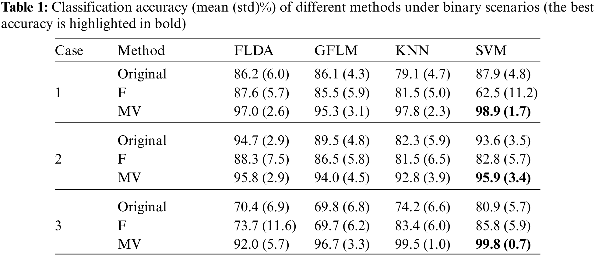
In Case 1, we mainly set two significant local coefficient features, which have a smaller variance than the other features. Similarly, in Case 3, we alternately set the variance sizes on the coefficients of the B-spline basis functions to generate data with local significant and confusing features. In general, setting disturbances on the coefficients is compatible with the two approaches, i.e., KNN and SVM. The penalized B-splines method can effectively smooth out some random noise and extract low-dimensional features. Therefore, in Cases 1 and 3, KNN and SVM can usually achieve higher classification accuracy than FLDA and GFLM. The MVSVM method achieve the best classification accuracy at 98.9%, 95.9%, and 99.8% in Cases 1, 2, and 3, respectively, followed by MVKNN and MVFLDA. Compared with the original classifiers, the F-score-based method exhibits instability, a notable drawback inherent in feature selection. In contrast, our proposed method not only demonstrates a substantial enhancement in classification performance but also ensures commendable stability over varying conditions.

Different from the above two cases, in Case 2, random noise is directly added to the smooth function to set different variances. It can be clearly found that significant features are positioned in the middle, while confusing features are situated at both ends of the curves. These settings are advantageous to FLDA, whose original classification accuracy can achieve 94.7%, which is better than GFLM, KNN, and SVM. In Case 2, it is evident that the F-score-based method fails to improve the classification performance, whereas our MV approach markedly enhances the classification accuracy of the original classifiers. The MVSVM attains the highest classification accuracy at 95.9% in Case 2, followed by MVFLDA.

In addition, we consider a multi-class classification scenario with the combination of three mean functions. Table 2 summarizes the classification accuracy (mean (std)%) of different methods under multi-class scenarios.

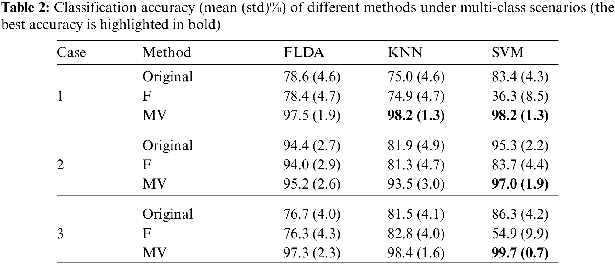
For the three cases, the F-score-based method could hardly improve the classification performance of the original classifier. In the FSVM, the F-score-based method filters out unimportant features, leading to loss of information and weakening the help of the RBF kernel. However, the MVSVM can achieve the best classification accuracy of 98.2%, 97.0%, and 99.7% in the three cases, respectively.

Based on the foregoing studies, the MV feature weighting method not only significantly enhances the classification performance of the original classifier but also exhibits heightened classification stability, as evidenced by a reduced standard deviation in classification accuracy. The more significant features within the dataset, the more effective our method becomes.

The principle of the F-statistic method is to filter features based on the F-statistic and a specified level of significance. The F-statistic methods can uncover the essential features of classification. After spline approximation or functional principal component decomposition, there are not many nuisance features for the functional data. The feature selection method based on F-statistics carries the risk of losing important information, leading to limited classification accuracy.

4  Application

We apply the proposed method to six time series data sets, which can be taken from http://www.timeseriesclassification.com. The detailed information on these data sets is listed in Table 3. The training samples of the six time series data sets are plotted in Fig. 2.

Figure 2: Training samples of the six time series data sets

The first example is the DodgerLoopGame traffic data, which is collected with the loop sensor installed on the ramp for the 101 North freeway in Los Angeles. This location is close to Dodgers Stadium. Therefore, the traffic is affected by the volume of visitors to the stadium. The curves in this dataset are categorized into two classes: Normal Day and Game Day. All samples with missing values in the DodgerLoopGame dataset have been excluded for ease of analysis.

The second example is the ECG200 data. Each series traces the electrical activity recorded during one heartbeat. The two classes are a normal heartbeat vs. a myocardial infarction event (heart attack due to prolonged cardiac ischemia).

The third example is the ECGFiveDays data, sourced from a 67-year-old male. The two classes correspond to two dates that the electrocardiogram (ECG) was recorded, which are five days apart: 12/11/1990 and 17/11/1990.

The fourth example is the PowerCons data, which encompasses individual household electric power consumption throughout the year. The data is categorized into two seasonal classes: Warm and cold. Classification is based on whether the power consumption is recorded during the warm seasons (from April to September) or the cold seasons (from October to March). Notably, the electric power consumption profiles exhibit distinct variations within each class. The dataset is sampled every ten minutes over one year.

The fifth example is the CBF data, which is a simulated data set. Data from each class are standard normal noise plus an offset term, which differs for each class.

The sixth example is the BME data, which is a synthetic data set with three classes: One class is characterized by a small positive bell arising at the initial period (Begin), one does not have any bell (Middle), one has a positive bell arising at the final period (End). All series are constituted by a central plate. The central plates may be positive or negative. The discriminant is the presence or absence of a positive peak, which is at the beginning or the end of the series.

In the application, we add supervised functional principal component analysis (sFPCA) [38] to compare the classification performance of binary data. We use the leading two functional principal components to get the classification result.

Table 4 summarizes the classification accuracy (%) of different methods under four binary classification time series data sets. For the DodgerLoopGame data, due to the presence of observational noise, our method does not lead to a significant improvement in GFLM and sFPCA. However, both MVKNN and MVSVM are significantly enhanced compared with the original classifier. The F-score-based method is ineffective for data with a high signal-to-noise ratio and lacking significant local features. In the case of the ECG200 dataset, the F-score-based method exhibits instability, whereas the MV method effectively preserves or enhances the classification performance. Notably, in this dataset, MVSVM attains the highest accuracy of 89.0%, closely approaching the performance of the best algorithm. For the ECGFiveDays data, the MV method substantially enhances the original performance. Specifically, MVSVM achieves an accuracy of 98.5%. For the PowerCons data, from the perspective of classification, the difference in the level of electricity consumption in different seasons is obvious and easy to classify. Our method can maintain a stable classification performance.

Table 5 summarizes the classification accuracy (%) of different methods under two multi-classification time series data sets. The CBF and BME are multi-classification data sets. For the CBF and BME data, our method can improve the performance of the original classifiers. The MVFLDA achieves the best accuracy of 94.6% in CBF data, and the MVSVM reaches the best accuracy of 88.0% in BME data.

The outcomes from all instances demonstrate that: First, the MV method can greatly enhance the contribution of important local features to classification; second, the MV method can be integrated with diverse classification methods to adapt to different data scenarios, enhancing classification performance while ensuring stability.

From Fig. 2, the smoothness of the BME curves is relatively high. Therefore, there is less information lost after extracting features through spline approximation. Moreover, the BME curves exhibit distinct segmented features, which are beneficial for enhancing the differences among different classes through feature weighting. These characteristics result in better classification performance of the data through the weighted method.

As shown in the outcomes, the F-statistic method often does not improve classification accuracy compared to the original methods. The principle of the F-statistic method is to filter features based on the F-statistic and a specified level of significance. The F-statistic method can uncover the essential features of classification. When there are a lot of nuisance features, it can filter them out to prevent overfitting. However, when there are not many nuisance features or the difference among F-statistics of the features is not significant, it carries the risk losing important information, leading to limited classification accuracy.

Additionally, when the class labels can be identified through linear features of functional explanatory variables, FLDA and GFLM may perform better. Otherwise, SVM may be better when the class labels need to be identified through the nonlinear features of the functional explanatory variables.

5  Conclusion

In this paper, we propose a mean-variance-based feature weighting method for curve classification. This method can be integrated with various functional classification methods. On the one hand, we use B-spline basis expansion to extract coefficient features and combine them with KNN and SVM. On the other hand, we treat the reconstructed functional data as features and use FLDA and GFLM for classification. An important advantage of this method is that the relative importance of each feature is considered in the classification rather than being dominated by confusing features. We demonstrate the classification performance on one-dimensional function curves. The proposed feature weighting approach can still work after tensor spline basis expansion for multi-dimensional functional data. When functional data appears sparse [39,40] or contains outliers [12,41], the feature weighting methods are attractive for future studies.

Our method did not utilize the class labels while extracting functional data features. Therefore, there may be situations where important features are lost or situations where there are too many nuisance features. At this point, the weighting method may not be effective. We suggest using supervised learning methods [42,43] to extract features to ensure the efficiency of feature weighting. In addition, we only weighted each feature separately and did not consider the correlation between features. This also affects the weighting effect to a certain extent. In addition, we only weighted each feature separately and did not consider the correlation between features. Further research is needed on assigning correlated weights based on the correlation of features.

Acknowledgement: None.

Funding Statement: This work is supported by the National Social Science Foundation of China (Grant No. 22BTJ035).

Author Contributions: Study conception and design: Chunzheng Cao; data collection: Sheng Zhou; analysis and interpretation of results: Zewen Zhang and Sheng Zhou; draft manuscript preparation: Chunzheng Cao, Sheng Zhou and Zewen Zhang. All authors reviewed the results and approved the final version of the manuscript.

Availability of Data and Materials: All publicly available datasets are used in the study.

Conflicts of Interest: The authors declare that they have no conflicts of interest to report regarding the present study.

References

1. J. O. Ramsay and B. W. Silverman, “Introduction,” in Functional Data Analysis, 2nd ed. New York, USA: Springer, 2005, vol. 1, pp. 1–18. [Google Scholar]

2. R. Blanquero, E. Carrizosa, A. Jiménez-Cordero, and B. Martín-Barragán, “Variable selection in classification for multivariate functional data,” Inf. Sci., vol. 481, no. 9, pp. 445–462, 2019. doi: 10.1016/j.ins.2018.12.060. [Google Scholar] [CrossRef]

3. S. Jiang, J. Cao, B. Rosner, and G. A. Colditz, “Supervised two-dimensional functional principal component analysis with time-to-event outcomes and mammogram imaging data,” Biometrics, vol. 79, no. 2, pp. 1359–1369, 2023. doi: 10.1111/biom.13611. [Google Scholar] [PubMed] [CrossRef]

4. G. E. Castro Guzman and A. Fujita, “Convolution-based linear discriminant analysis for functional data classification,” Inf. Sci., vol. 581, pp. 469–478, 2021. doi: 10.1016/j.ins.2021.09.057. [Google Scholar] [CrossRef]

5. A. Weishampel, A. M. Staicu, and W. Rand, “Classification of social media users with generalized functional data analysis,” Comput. Stat. Data Anal., vol. 179, pp. 107647, 2023. doi: 10.1016/j.csda.2022.107647. [Google Scholar] [CrossRef]

6. M. Mutis, U. Beyaztas, G. G. Simsek, and H. Shang, “A robust scalar-on-function logistic regression for classification,” Commun. Stat. Theory Methods, vol. 52, no. 23, pp. 8538–8554, 2023. doi: 10.1080/03610926.2022.2065018. [Google Scholar] [CrossRef]

7. H. G. Müller and U. Stadtmüller, “Generalized functional linear models,” Ann. Stat., vol. 33, no. 2, pp. 774–805, 2005. doi: 10.1214/009053604000001156. [Google Scholar] [CrossRef]

8. F. Chamroukhi and H. D. Nguyen, “Model-based clustering and classification of functional data,” Wiley Interdis. Rev.: Data Mining Knowl. Dis., vol. 9, no. 4, pp. e1298, 2019. doi: 10.1002/widm.1298. [Google Scholar] [CrossRef]

9. G. M. James and T. J. Hastie, “Functional linear discriminant analysis for irregularly sampled curves,” J. Royal Stat. Soci.: Series B (Stat. Method.), vol. 63, no. 3, pp. 533–550, 2002. doi: 10.1111/1467-9868.00297. [Google Scholar] [CrossRef]

10. Y. C. Zhang and L. Sakhanenko, “The naive Bayes classifier for functional data,” Stat. Probab. Lett., vol. 152, no. 16–17, pp. 137–146, 2019. doi: 10.1016/j.spl.2019.04.017. [Google Scholar] [CrossRef]

11. A. Chatterjee, S. Mazumder, and K. Das, “Functional classwise principal component analysis: A classification framework for functional data analysis,” Data Min. Knowl. Discov., vol. 37, no. 2, pp. 552–594, 2023. doi: 10.1007/s10618-022-00898-1. [Google Scholar] [CrossRef]

12. C. Cao, X. Liu, S. Cao, and J. Q. Shi, “Joint classification and prediction of random curves using heavy-tailed process functional regression,” Pattern Recognit., vol. 136, no. 1, pp. 109213, 2023. doi: 10.1016/j.patcog.2022.109213. [Google Scholar] [CrossRef]

13. B. Li and Q. Yu, “Classification of functional data: A segmentation approach,” Comput. Stat. Data Anal., vol. 52, no. 10, pp. 4790–4800, 2008. doi: 10.1016/j.csda.2008.03.024. [Google Scholar] [CrossRef]

14. S. Gardner-Lubbe, “Linear discriminant analysis for multiple functional data analysis,” J. Appl. Stat., vol. 48, no. 11, pp. 1917–1933, 2021. doi: 10.1080/02664763.2020.1780569. [Google Scholar] [PubMed] [CrossRef]

15. A. Jiménez-Cordero and S. Maldonado, “Automatic feature scaling and selection for support vector machine classification with functional data,” Appl. Intell., vol. 51, no. 1, pp. 161–184, 2021. doi: 10.1007/s10489-020-01765-6. [Google Scholar] [CrossRef]

16. X. Dai, H. G. Müller, and F. Yao, “Optimal bayes classifiers for functional data and density ratios,” Biometrika, vol. 104, no. 3, pp. 545–560, 2017. doi: 10.1093/biomet/asx024. [Google Scholar] [CrossRef]

17. P. Kokoszka and R. Kulik, “Principal component analysis of infinite variance functional data,” J. Multivar. Anal., vol. 193, no. 94, pp. 105123, 2023. doi: 10.1016/j.jmva.2022.105123. [Google Scholar] [CrossRef]

18. R. Zhong, S. Liu, H. Li, and J. Zhang, “Sparse logistic functional principal component analysis for binary data,” Stat. Comput., vol. 33, no. 15, pp. 503, 2023. doi: 10.1007/s11222-022-10190-3. [Google Scholar] [CrossRef]

19. P. H. C. Eilers and B. D. Marx, “Flexible smoothing with B-splines and penalties,” Stat. Sci., vol. 11, no. 2, pp. 89–121, 1996. doi: 10.1214/ss/1038425655. [Google Scholar] [CrossRef]

20. P. H. C. Eilers and B. D. Marx, “Splines, knots, and penalties,” Wiley Interdis. Rev.: Comput. Stat., vol. 2, no. 6, pp. 637–653, 2010. doi: 10.1002/wics.125. [Google Scholar] [CrossRef]

21. C. Iorio, G. Frasso, A. D’Ambrosio, and R. Siciliano, “Parsimonious time series clustering using P-splines,” Expert. Syst. Appl., vol. 52, no. 3, pp. 26–38, 2016. doi: 10.1016/j.eswa.2016.01.004. [Google Scholar] [CrossRef]

22. M. López, J. Martínez, J. M. Matías, J. Taboada, and J. A. Vilán, “Functional classification of ornamental stone using machine learning techniques,” J. Comput. Appl. Math., vol. 234, no. 4, pp. 1338–1345, 2010. doi: 10.1016/j.cam.2010.01.054. [Google Scholar] [CrossRef]

23. G. Bhattacharya, K. Ghosh, and A. S. Chowdhury, “Granger causality driven AHP for feature weighted kNN,” Pattern Recognit., vol. 66, no. 6, pp. 425–436, 2017. doi: 10.1016/j.patcog.2017.01.018. [Google Scholar] [CrossRef]

24. Y. Chen and Y. Hao, “A feature weighted support vector machine and k-nearest neighbor algorithm for stock market indices prediction,” Expert. Syst. Appl., vol. 80, pp. 340–355, 2017. doi: 10.1016/j.eswa.2017.02.044. [Google Scholar] [CrossRef]

25. K. Zheng and X. Wang, “Feature selection method with joint maximal information entropy between features and class,” Pattern Recognit., vol. 77, no. 6, pp. 20–29, 2018. doi: 10.1016/j.patcog.2017.12.008. [Google Scholar] [CrossRef]

26. S. Sharmin, M. Shoyaib, A. A. Ali, M. A. H. Khan, and O. Chae, “Simultaneous feature selection and discretization based on mutual information,” Pattern Recognit., vol. 91, no. 26, pp. 162–174, 2019. doi: 10.1016/j.patcog.2019.02.016. [Google Scholar] [CrossRef]

27. I. Niño-Adan, D. Manjarres, I. Landa-Torres, and E. Portillo, “Feature weighting methods: A review,” Expert. Syst. Appl., vol. 184, no. 2, pp. 115424, 2021. doi: 10.1016/j.eswa.2021.115424. [Google Scholar] [CrossRef]

28. P. Wei, Z. Lu, and J. Song, “Variable importance analysis: A comprehensive review,” Reliab. Eng. Syst. Safety, vol. 142, no. 3, pp. 399–432, 2015. doi: 10.1016/j.ress.2015.05.018. [Google Scholar] [CrossRef]

29. P. J. García-Laencina, J. L. Sancho-Gómez, A. R. Figueiras-Vidal, and M. Verleysen, “K nearest neighbours with mutual information for simultaneous classification and missing data imputation,” Neurocomputing, vol. 72, no. 7–9, pp. 1483–1493, 2009. doi: 10.1016/j.neucom.2008.11.026. [Google Scholar] [CrossRef]

30. H. Xing, M. Ha, B. Hu, and D. Tian, “Linear feature-weighted support vector machine,” Fuzzy Inf. Eng., vol. 1, no. 3, pp. 289–305, 2009. doi: 10.1007/s12543-009-0022-0. [Google Scholar] [CrossRef]

31. L. Jiang, L. Zhang, C. Li, and J. Wu, “A correlation-based feature weighting filter for naive bayes,” IEEE Trans. Knowl. Data Eng., vol. 31, no. 2, pp. 201–213, 2019. doi: 10.1109/TKDE.2018.2836440. [Google Scholar] [CrossRef]

32. S. F. Hussain, “A novel robust kernel for classifying high-dimensional data using support vector machines,” Expert. Syst. Appl., vol. 131, no. 6, pp. 116–131, 2019. doi: 10.1016/j.eswa.2019.04.037. [Google Scholar] [CrossRef]

33. H. Wu, X. Gu, and Y. Gu, “Balancing between over-weighting and under-weighting in supervised term weighting,” Inf. Process. Manag., vol. 53, no. 2, pp. 547–557, 2017. doi: 10.1016/j.ipm.2016.10.003. [Google Scholar] [CrossRef]

34. J. Chang, “Functional data classification using the rotation forest method combined with the patch selection,” Commun. Stat.-Simul. C., vol. 52, no. 7, pp. 3365–3378, 2023. doi: 10.1080/03610918.2023.2205619. [Google Scholar] [CrossRef]

35. G. Frasso and P. H. C. Eilers, “L-and V-curves for optimal smoothing,” Stat. Model., vol. 15, no. 1, pp. 91–111, 2014. doi: 10.1177/1471082X14549288. [Google Scholar] [CrossRef]

36. P. C. Hansen, “Analysis of discrete ill-posed problems by means of the L-curve,” SIAM Rev., vol. 34, no. 4, pp. 561–580, 1992. doi: 10.1137/1034115. [Google Scholar] [CrossRef]

37. S. Ding, “Feature selection based F-score and ACO algorithm in support vector machine,” presented at the 2009 Second Int. Symp. Knowl. Acquis. Model., Wuhan, China, 2009, pp. 19–23. doi: 10.1109/KAM.2009.137. [Google Scholar] [CrossRef]

38. Y. Nie, L. Wang, B. Liu, and J. Cao, “Supervised functional principal component analysis,” Stat. Comput., vol. 28, no. 3, pp. 713–723, 2018. doi: 10.1007/s11222-017-9758-2. [Google Scholar] [CrossRef]

39. F. Yao, H. G. Müller, and J. L. Wang, “Functional data analysis for sparse longitudinal data,” J. Am. Stat. Assoc., vol. 100, no. 470, pp. 577–590, 2005. doi: 10.1198/016214504000001745. [Google Scholar] [CrossRef]

40. Y. Park, H. Kim, and Y. Lim, “Functional principal component analysis for partially observed elliptical process,” Comput. Stat. Data Anal., vol. 184, no. 537, pp. 107745, 2023. doi: 10.1016/j.csda.2023.107745. [Google Scholar] [CrossRef]

41. H. Shi and J. Cao, “Robust functional principal component analysis based on a new regression framework,” J. Agric. Biol. Envi. Stat., vol. 27, no. 3, pp. 523–543, 2022. doi: 10.1007/s13253-022-00495-1. [Google Scholar] [CrossRef]

42. Z. Ye, J. Chen, H. Li, Y. Wei, G. Xiao and J. A. Benediktsson, “Supervised functional data discriminant analysis for hyperspectral image classification,” IEEE Trans. Geosci. Remote Sens., vol. 58, no. 2, pp. 841–851, 2020. doi: 10.1109/TGRS.2019.2940991. [Google Scholar] [CrossRef]

43. F. Maturo and R. Verde, “Supervised classification of curves via a combined use of functional data analysis and tree-based methods,” Comput. Stat., vol. 38, no. 1, pp. 419–459, 2023. doi: 10.1007/s00180-022-01236-1. [Google Scholar] [CrossRef]