Low-Brightness Object Recognition Based on Deep Learning

1  Introduction

In recent years, the success of object recognition detection rates has been significant, particularly in well-lit environments where systems like Faster R-CNN [1], You Only Look Once version 4 (YOLOv4) [2], Single Shot Object Detector (SSD) [3], and others can achieve high accuracy through training. However, under insufficient lighting conditions, the success rate of image recognition significantly diminishes. In all-weather environments, scenarios of compromised object recognition exist due to inadequate light, such as nighttime, dense fog, and overcast days. Insufficient light at night creates a low-light environment, resulting in issues such as low brightness, low contrast, and noise in images.

The objective of this study is to utilize artificial intelligence for the development of a recognition system capable of functioning under different lighting conditions, eliminating the need for semantic segmentation of images to acquire scene parsing information, thus addressing challenges in nighttime or low-light image recognition. Therefore, this study proposes incorporating depth information into image signals, substituting part of the image signal with depth information to achieve three-channel signals akin to those in typical true color (RGB) images. By training and recognizing images with these adjusted image components, rapid nighttime or low-light image recognition results can be achieved. The experimental environment for this study involves indoor imagery, utilizing light adjustments to simulate the differences between daytime and nighttime images. The aim is to address image recognition issues throughout the whole day, enabling the system to operate seamlessly during both daytime and nighttime. The rest of the paper is structured as follows. A brief literature review is presented in Section 2. The materials and methods are described in Section 3, and the proposed image processing methods are also described in this section. The experimental results and conclusion are presented in Sections 4 and 5, respectively.

2  Literature Review

Addressing the challenges of image detection in low-light environments, especially applying artificial intelligence techniques to machine vision and object recognition systems, can enhance nighttime surveillance quality and also contribute to traffic safety in driving scenarios. Nevertheless, current datasets, such as the ImageNet dataset [4] and the Common Objects in Context (COCO) dataset [5], predominantly comprise well-lit images. Even if dark images are present, their quantity is limited, making it challenging to use their results for training and research. In low-light conditions, insufficient reflected light leads to uneven brightness, resulting in significant black areas and noise in images, making it difficult to detect object details. Therefore, there are approximately four main approaches for nighttime or low-light image recognition, which will be explained and analyzed below.

The first approach of nighttime image recognition involves using infrared images for nighttime recognition as infrared images are not affected by visible light. However, infrared images are typically single-channel images, leading to issues such as low contrast and blurriness. Training YOLOv4 directly with infrared images for object recognition yields unsatisfactory results because infrared images still lack sufficient features for effective detection. Therefore, Dai et al. [6] proposed the use of a Near Infrared (NIR) camera with a visible-spectrum (VIS) filter and a fill-light device as the camera and light source. They utilized a customized 9-layer convolutional neural network (CNN) model for pedestrian recognition, and during the training phase, manually separating background photos from pedestrian photos was necessary to achieve recognition accuracy. However, due to the additional light source and the use of a NIR camera with a VIS filter, as well as the need for pre-separation of photos and backgrounds, significant time is required for preprocessing.

The second approach is image enhancement, which transforms low-light images into ones resembling daytime images through enhancement techniques, thus improving recognition rates. The most intuitive method in image enhancement is histogram equalization [7], which redistributes the histogram of image intensities to become more uniform, thereby enhancing the image’s contrast. However, histogram equalization often leads to excessive enhancement, causing the loss of details in the image. Another approach is gamma correction, involving editing the gamma curve of an image. This method applies non-linear color editing to the image, detecting the dark and light portions of the image signal and increasing their ratio to enhance the overall image contrast. However, the results of this approach in nighttime object detection are not satisfactory. In current practices, many image enhancement approaches are based on the Retinex theory [8]. The Retinex theory analyzes and adjusts the brightness distribution of an image, aiming to mimic the adaptability of the human visual system to changes in illumination. Inspired by this theory, several image enhancement algorithms have been proposed in recent years. RetinexNet [9] utilizes DecomNet to decompose low-light images, estimate the illumination image, and then enhance the illumination image using EnhanceNet. Finally, by employing pixel-wise multiplication, the illumination image and reflectance image are reconstructed into a new image, which can enhance image recognition rates. RetiNex-Robust [10] introduces a noise term into the classical model, transforming the input image after subtracting the noise term to obtain a new image. Low-light image enhancement (LIME) [11] constructs an illumination map by finding the maximum values in the image for enhancement. However, images enhanced using these techniques may not outperform those trained on original data. While image enhancement has a powerful effect on human vision, it may not provide sufficient features for the goals of computer vision. Xiao et al. [12] tested three brightness enhancement algorithms on real low-light scenes, and all three methods resulted in images where targets were not detected. Therefore, using brightness enhancement algorithms alone in low-light scenarios may not necessarily achieve better detection outcomes.

The third approach involves using Generative Adversarial Networks (GANs) to transform nighttime images into fake daytime images to address nighttime recognition issues. In the study by Tan et al. [13], issues related to nighttime driving are addressed by combining features learned from overexposed images, caused by factors such as streetlights and car lights, with features from underexposed images using deep learning methods. Additionally, Chia et al. [14] propose using GANs [15] to transform nighttime images into pseudo-daytime images, aiming to resolve nighttime recognition challenges. As object detection in RGB images is prone to lighting influences, one approach to address nighttime detection problems is through style transfer, translating nighttime images into daytime images. GANs [15] are a form of unsupervised learning, and the translation of images can be categorized into two types. The first is paired image translation, such as converting daytime street scenes into nighttime scenes, which requires collecting identical images at the same location. However, obtaining such paired images is challenging, making data collection for training difficult. Therefore, Lee et al. [16] use GAN technology to transform daytime images into synthetically generated nighttime images to augment the dataset. Another approach, proposed by Zhu et al. [17], involves non-paired image translation applied to style transfer. This method only requires collecting individual daytime and nighttime images without the need for paired images for translation. In the paper of Chia et al. [14], CycleGAN is used to transform images from nighttime to pseudo-daytime. However, during the translation of nighttime images into pseudo-daytime images, undesirable results may occur, leading to distortions where many objects fail to retain their original states. Lakmal et al. [18] propose training a supervised GAN model on a pixel-to-pixel night-to-day image dataset, which improves image recognition performance, but the results still cannot fully address nighttime image recognition. Cheng et al. [19] combine attention mechanisms and multiscale feature fusion to improve the generator network for noise reduction, yet its effectiveness still falls short of achieving efficient nighttime image recognition.

The fourth approach involves initially segmenting the image to reduce noise in nighttime images, which can enhance the recognition rate. Image segmentation, as a preprocessing step for image recognition, can reduce background interference, minimize the impact of noise, increase the contrast between targets and backgrounds, and enhance the distinctive features of the target of interest. When segmenting RGB images, the segmentation is typically performed based on the contours of objects, utilizing methods such as Canny edge detection [20], Prewitt operator [21], Laplacian operator [22], etc. However, contour-based methods rely on brightness or color variations to identify targets, and their effectiveness diminishes in slightly complex environments or low-light scenes. Ester et al. proposed a density-based clustering algorithm called Density-Based Spatial Clustering of Applications with Noise (DBSCAN) [23]. While DBSCAN can classify clusters without specifying the number of clusters, it incurs a higher time cost when dealing with larger datasets, as it requires calculating the density between each pair of pixels. In comparison, the k-means method proposed by MacQueen [24] uses Euclidean distance to calculate the distance from each point to the cluster center, allowing for the adaptive determination of a suitable k value. In addition to image segmentation, semantic segmentation is currently employed in the field of computer vision for scene parsing. This process involves classifying each pixel in an image into its corresponding object, wherein scene parsing provides contextual information to enhance the accuracy of deep learning models used for this purpose. Alid et al. [25] propose the utilization of the Fully Convolutional Network (FCN-8) architecture for effective semantic segmentation in scene parsing. However, the primary focus has been on daytime scenes, highlighting the necessity of effectively addressing nighttime scenes to enhance the safety of nighttime autonomous driving. Tan et al. [13] introduce the use of a large dataset comprising real nighttime images with detailed semantic annotations to tackle the challenge of nighttime scene parsing. They incorporated an exposure guidance layer to integrate semantic label maps with exposure maps, whereby exposure features are learned to improve the scene parsing segmentation process. Although their research significantly enhanced nighttime scene parsing performance, their model may fail in cases where underexposed regions are extensive. Xie et al. [26] identify significant disparities in image frequency distributions between daytime and nighttime scenes. Consequently, they proposed leveraging image frequency distributions for nighttime scene parsing. Initially, they employed a learnable frequency encoder to establish a model of the relationship between different frequency coefficients. Subsequently, they utilized a spatial frequency fusion module to amalgamate spatial and frequency information, thereby guiding the extraction of spatial context features.

Summing up the aforementioned approaches for nighttime image recognition, whether image enhancement, infrared image recognition, GAN transformation into fake daytime images, or image segmentation to remove background noise, their effectiveness in nighttime image recognition remains limited. In addition, there is also research on integrating RGB and thermal imaging for person recognition [27]. This study introduces YOLO4-T, which involves converting the RGB color space into HSV (hue, saturation, value). In this process, the 8-bit thermal image, T, replaces the value component, which represents brightness. This transformation results in an HST space (hue, saturation, thermal) for recognition. However, the recognition rate of the HST approach is only 0.65 for nighttime images.

3  Materials and Methods

The experimental setup for this study utilized the 2021 ROG Zephyrus G14, equipped with an Nvidia RTX3060 GPU, and the Windows operating system with Anaconda. The research was conducted using PyTorch. The study incorporated the Intel RealSense L515 LiDAR depth camera, as shown in Fig. 1. The RGB color image resolution is 1920 × 1080, sampled at a rate of 30 fps, while the depth image resolution is 1024 × 768, also sampled at 30 fps. The minimum depth distance is 0.25 m, and the usable distance ranges from 0.25 to 9 m.

Figure 1: Intel RealSense L515 idar depth camera

3.1 Image Affine Transformation

The size of both the RGB and depth images in the experiment is 640 × 480. However, due to the positional difference between the RGB and depth lenses in the Intel RealSense L515 Lidar depth camera, alignment is required before image generation; as illustrated in Fig. 2a represents the RGB image; Fig. 2b shows the unaligned depth image and Fig. 2c displays the aligned image. Misalignment can result in incorrect depth information for the RGB image. In RGB images of Fig. 2a, we use a green box to represent the size and position of a person. Similarly, in the depth images in Fig. 2b, the green box of the same size and position indicates that the depth image shifts to the left and downwards. The distance between the person in the depth image and the green box is indicated by yellow arrows. Therefore, after aligning and correcting the images, the green box around the person in the depth image in Fig. 2c and the RGB image in Fig. 2a are perfectly aligned. The images Figs. 2b and 2c below are represented as 16-bit integers in the range of 0 to 255, with color added to indicate distance intervals. The closer distances are represented by a light blue color series, while the farther distances are depicted by a color series ranging from red to yellow. The dark blue portions indicate areas where no depth values were read. The affine transformation is used for RGB image and depth image. In Eq. (1), (x, y) are the coordinates of the RGB in the original image, (x′, y′) are the coordinates of depth imaging, b0 and b1 are offset, and b0 is along the coordinate X. The direction is translated, and b1 is translated along the coordinate Y direction to generate (x′, y′). Among them, a00 and a11 are the ratios obtained by the align_to function of the software development kit (SDK), a01 and a10 are 0, which are expressed in matrix form, such as Eq. (2). Using the translation variable between the two images to adjust b0 and b1, the color image and depth image can be aligned and the result of the depth image after the affine transformation is shown in Fig. 2c. Therefore, it is necessary to align the depth image with the RGB image for further research.

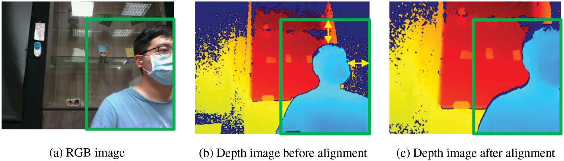
Figure 2: Differences before and after alignment of RGB images and depth image

x′=a00x+a01y+b0y′=a10x+a11y+b1(1)

[x′y′]=[a0000a11]×[xy]+[b0b1](2)

3.2 System Design

The proposed architecture of the system is illustrated in Fig. 3. When performing object detection during the daytime, where lighting conditions are sufficient, the detection process proceeds normally. However, in low-light environments, the detection effectiveness is not as prominent as during the daytime. In this study, preprocessing is applied to both depth and RGB images before recognition, aiming to enhance the recognition performance in low-light conditions. In Fig. 3, I indicates RGB images, D represents depth images, d signifies normal brightness images, n denotes nighttime images, and t is the input image number. L represents the average brightness of the image as shown in Eq. (3), It (h, w) indicate the pixels of image (h, w) and the H and W are the height and width of the image, respectively. LT represents the critical threshold for determining image brightness. In the experiment, LT is set to 25, as shown in Eq. (4). The process in Fig. 3 is represented by colored boxes, with blue boxes indicating the input image. The primary judgment is made based on the average brightness value L of the RGB image. This judgment is represented by a red box. When the average brightness value L is greater than or equal to the brightness threshold LT, it is classified as daytime (day), corresponding to normal brightness images and the image recognition system (green box) operates using the RGB image. When the average brightness value L is less than the brightness threshold LT, it is classified as nighttime (night), representing low-brightness images. In such cases, both the RGB image and the depth image are used as inputs, and the proposed image processing method in this study is applied (purple box), before proceeding to the image recognition system (green box). The image recognition results are indicated by the yellow box. The standard deviation is a measure of the degree of brightness variation, as shown in Eq. (5). σ represents the standard deviation, calculated by summing the squared differences between each pixel’s brightness value and the average brightness, dividing by the total number of pixels in the image, and taking the square root to obtain the standard deviation value.

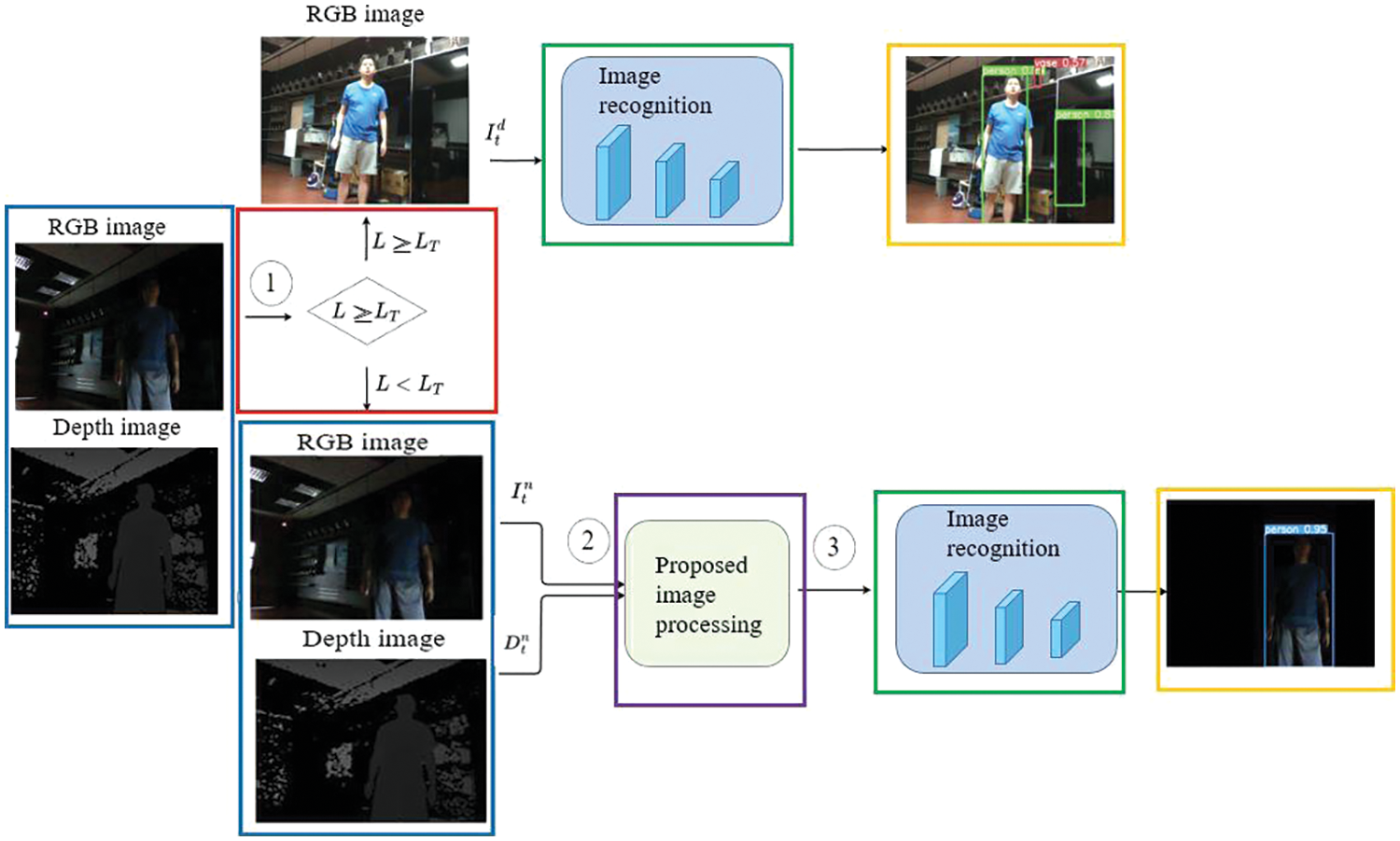
Figure 3: System flow chart

L=∑h∑wIt(h,w)/(H×W)(3)

{L≥LT,dayL<LT,night(4)

σ=∑h∑w(It(h,w)−L)2/(H×W)(5)

The steps in Fig. 3 will be explained in three processes. In the first process ① of Fig. 3, marked in a red box, after reading the image, the system uses RGB images to determine whether it is a normal or low-brightness scene. In the case of a normal brightness scene, the system directly uses RGB images for recognition. If it is a low-brightness image, it needs to be processed through image preprocessing for better recognition results. The determination of image brightness is based on the average brightness and standard deviation of the image. Through the standard deviation, the contrast of brightness values in the image can be assessed. When the standard deviation is larger, there is greater brightness variation, and shadows may exist, especially when the average brightness is high. Conversely, when the standard deviation is small, brightness variation is minimal, and if the average brightness is also low, it can be considered as low brightness. In this study, images with an average brightness below 25 are classified as low-brightness images. The second process ② of Fig. 3, marked in a purple box, will be discussed in the next section, and in the third process ③ of Fig. 3, marked in a green box, YOLOv4 will be used as the object detection method as shown in Fig. 4. The YOLOv4 model consists primarily of three architectures: Backbone, Neck, and Head. Utilizing SPP (Spatial Pyramid Pooling) combined with PaNet (Path Aggregation Network) in the Neck allows for better feature fusion, resulting in improved efficiency for rapid object detection.

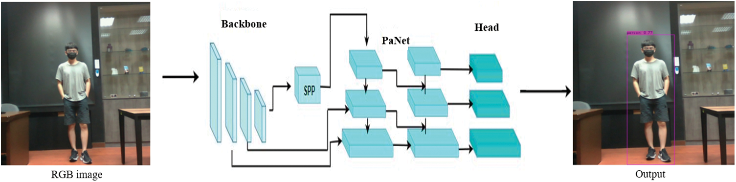
Figure 4: YOLO v4 structure for object recognition

Fig. 5a has an average brightness of 9.05 and a standard deviation of 16.37. Fig. 5b illustrates the brightness distribution of image Fig. 5a, with the red dashed line representing the average value. Fig. 5c is an image under normal brightness with an average brightness of 86.10 and a standard deviation of 48.80. Fig. 5d shows the brightness distribution of image Fig. 5c, with the red line indicating the average value.

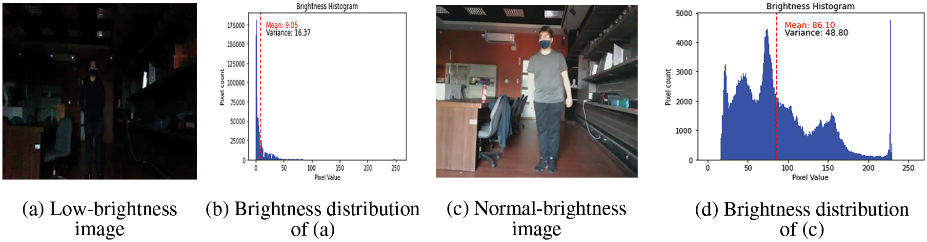
Figure 5: Brightness distribution of the image

3.3 Proposed Image Processing

In the flow ② of Fig. 3, three methods are employed in this study. The first method is the SD method (segmentation with depth image) which involves recognition using depth image segmentation. The second method is the HDV method (hue, depth, value) which combines RGB images converted to HSV images, where HSV represents hue, saturation, and value, a color space widely used in image processing and computer graphics. Subsequently, the HSV image is merged with depth information, D, to form an HDV image for recognition. The third method is the HSD method (hue, saturation, depth) which similarly combines RGB images converted to HSV images with depth images D to form HSD images for recognition.

3.3.1 SD Method

Fig. 6 depicts the steps of the SD method. Initially, the depth image undergoes processing within the purple box, utilizing k-means clustering and the eight-connectivity method to eliminate the background and produce a mask. This mask is subsequently merged with the RGB image through an AND operation, yielding an RGB image devoid of background for recognition. Following this, object recognition takes place within the green box, with the outcomes presented in the yellow box.

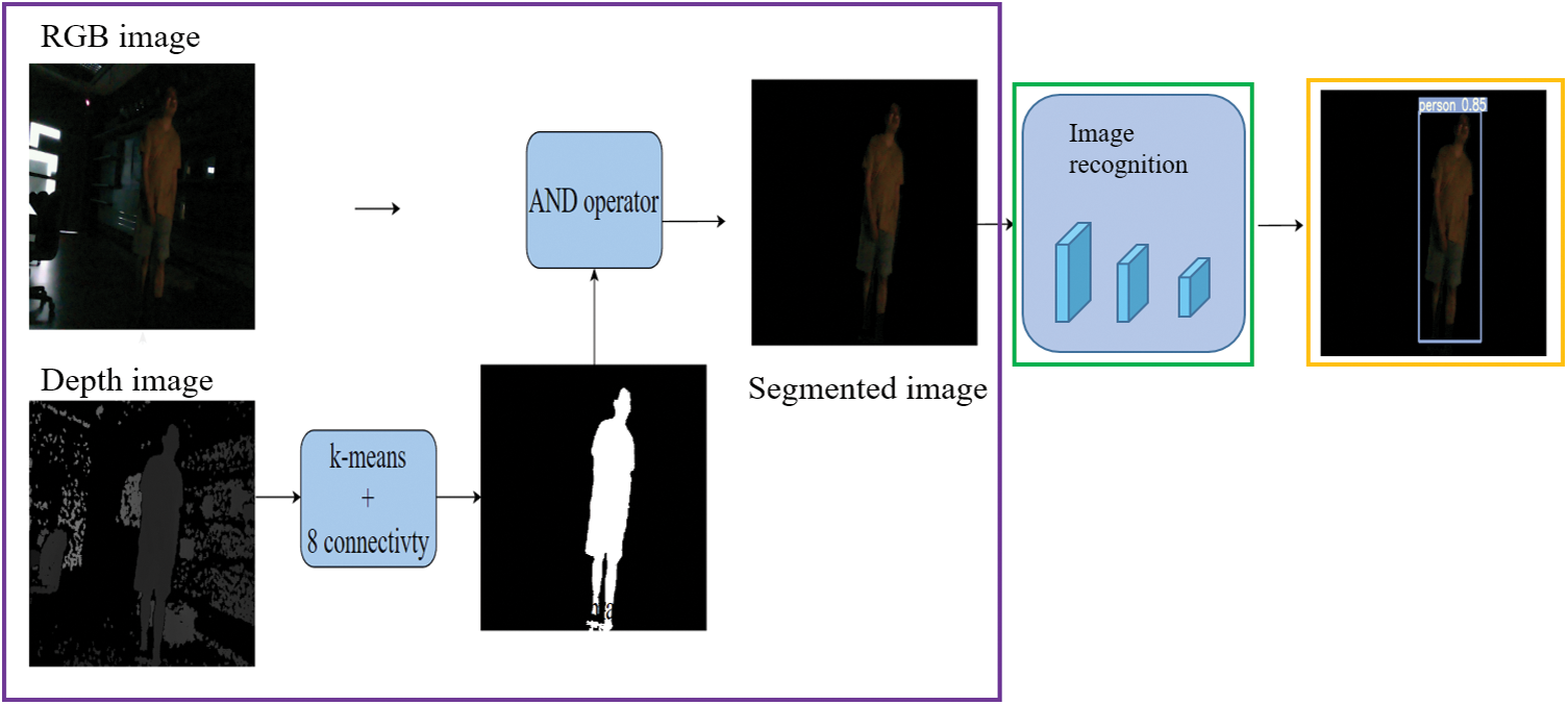
Figure 6: SD method

Fig. 7a shows an RGB image, while Fig. 7b represents the depth image processed through k-means clustering. After clustering, the minimum depth value in each cluster is identified, and a mask is created based on the cluster with the minimum depth value. Therefore, after clustering, by finding the minimum depth value in each cluster and creating a mask based on the identified cluster, object detection is performed on the connected components of the resulting masked image as shown in Fig. 7c. Finally, the final segmentation result is shown in Fig. 7d using the eight-connectivity method to calculate the maximum area within the mask.

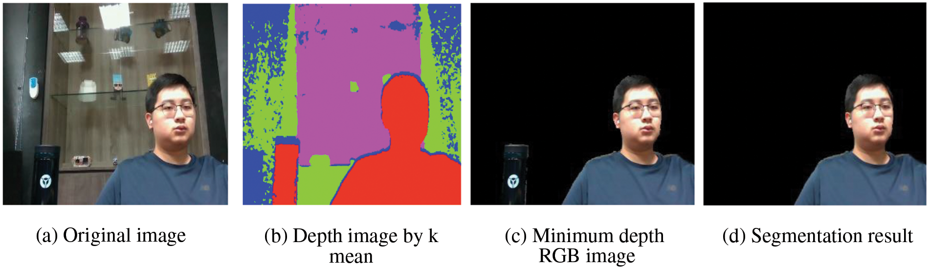
Figure 7: SD method process and result

During training, two different images are used: The model is trained once with the original image and again with the segmented image. Fig. 8a represents the brightness distribution of the image, with an average brightness of 15.81 and a standard deviation of 39.31. Fig. 8b shows the results of training the model with the original image, where no target is detected, while Fig. 8c displays the result of training the model with the segmented image and recognition rate for the target “person” as 0.92. The results indicate that by segmenting the images and reducing background interference, the system can focus on the target objects, enhancing the accuracy of recognition.

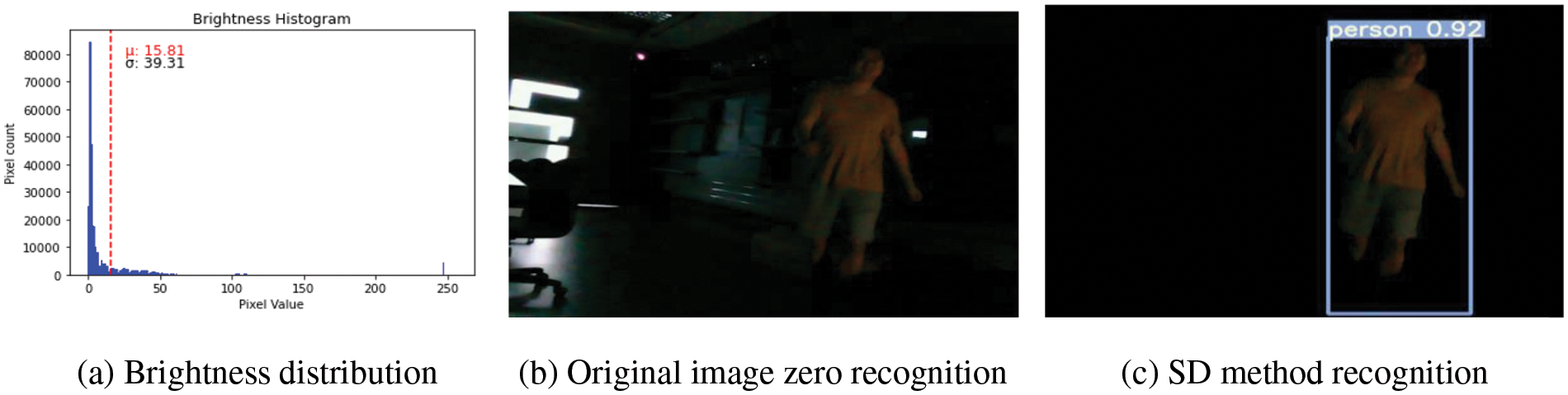
Figure 8: SD method recognition

3.3.2 HDV Method

The second method is the HDV method, where HDV represents hue, depth, and value. Initially, the RGB image is transformed into an HSV image. Then, the S-channel image is replaced with the depth image D, while preserving the original H and V channels to form HDV images. Since the depth information is 16-bit data, to fit the channel of 8-bit, the transformation from 16-bit to 8-bit is stated in Eq. (6). The HDV method is illustrated in Figs. 9a and 9b. The purple box in Fig. 9a represents the HDV method, where the RGB image is converted to an HSV image, and then the S channel of the image is replaced with the depth image, D. Object recognition is performed within the green box, and the results are presented in the yellow box. Conducting experiments using the HDV method, Fig. 10a depicts the brightness distribution of the RGB image, with an average brightness of 15.81 and a standard deviation of 39.31. Fig. 10b represents the RGB image, while Fig. 10c shows the result of recognition after training with the HDV image, achieving a recognition rate of 0.90.

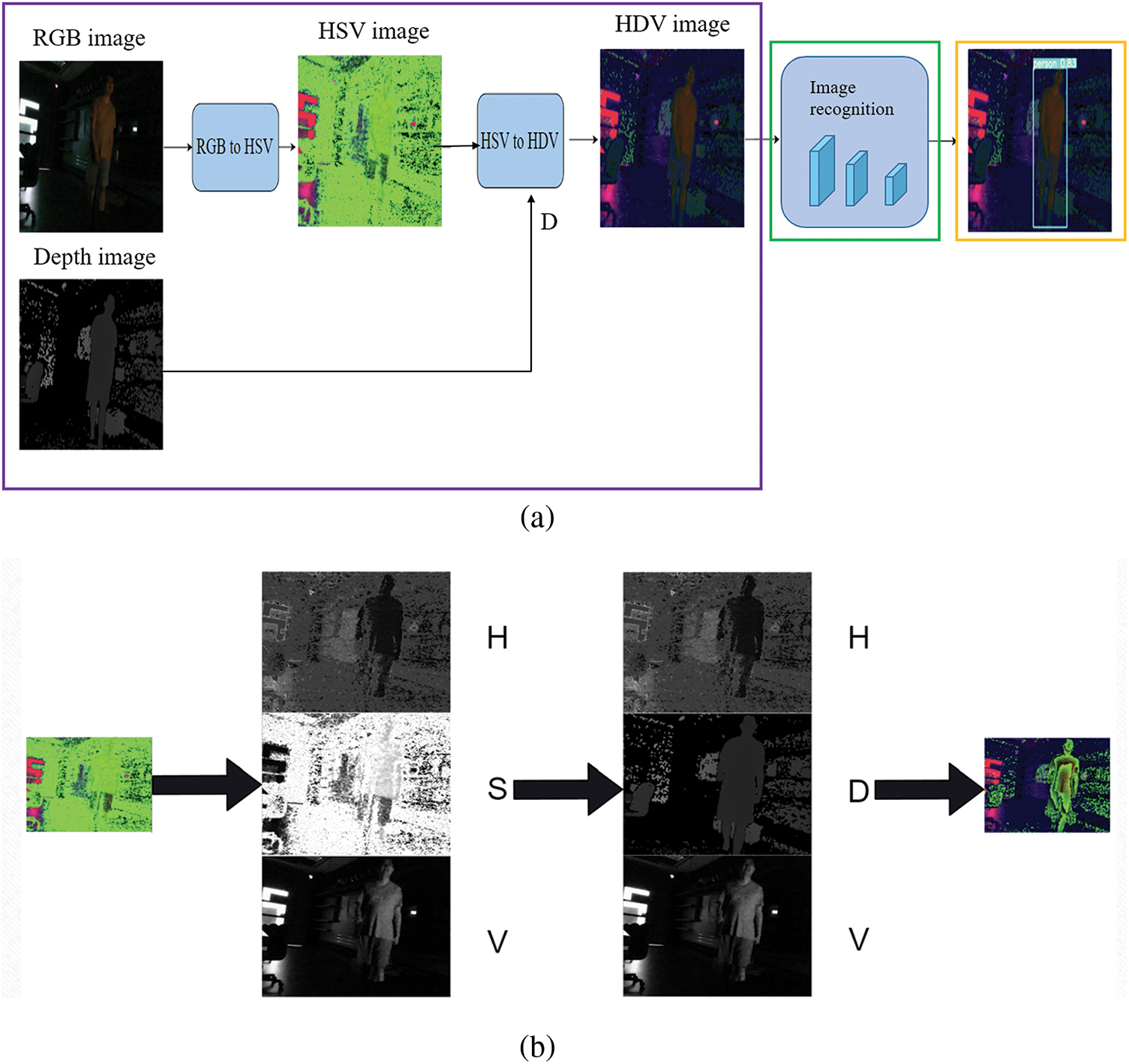
Figure 9: HDV method

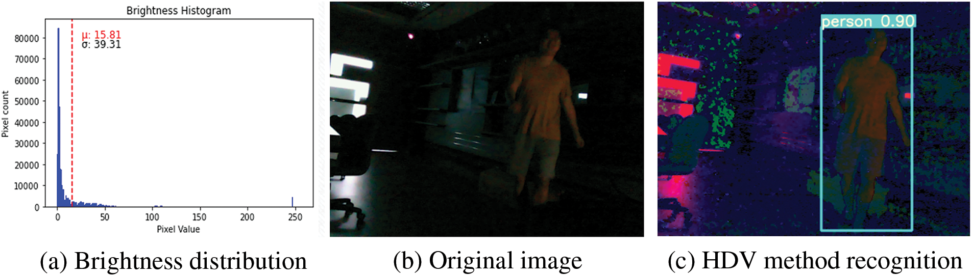
Figure 10: HDV method recognition

D=depth216−1⋅(28−1)(6)

3.3.3 HSD Method

The third method is the HSD method, which is similar to HDV method, where the RGB image is transformed into an HSV image. In this process, the V-channel is replaced with the depth image D by Eq. (6), while preserving the original H and S channels. The HSD method is illustrated in Figs. 11a and 11b. Similarly, the purple box in Fig. 11a represents the HSD method, where the RGB image is converted to an HSV image, and then the V channel of the image is replaced with the depth image, D. The green box indicates object recognition, and the results are presented in the yellow box. Using this method to conduct experiments, Fig. 12a depicts the brightness distribution of the RGB image, with an average brightness of 15.81 and a standard deviation of 39.31. Fig. 12b represents the RGB image, while Fig. 12c shows the result of recognition after training with the HSD image, achieving a recognition rate of 0.94.

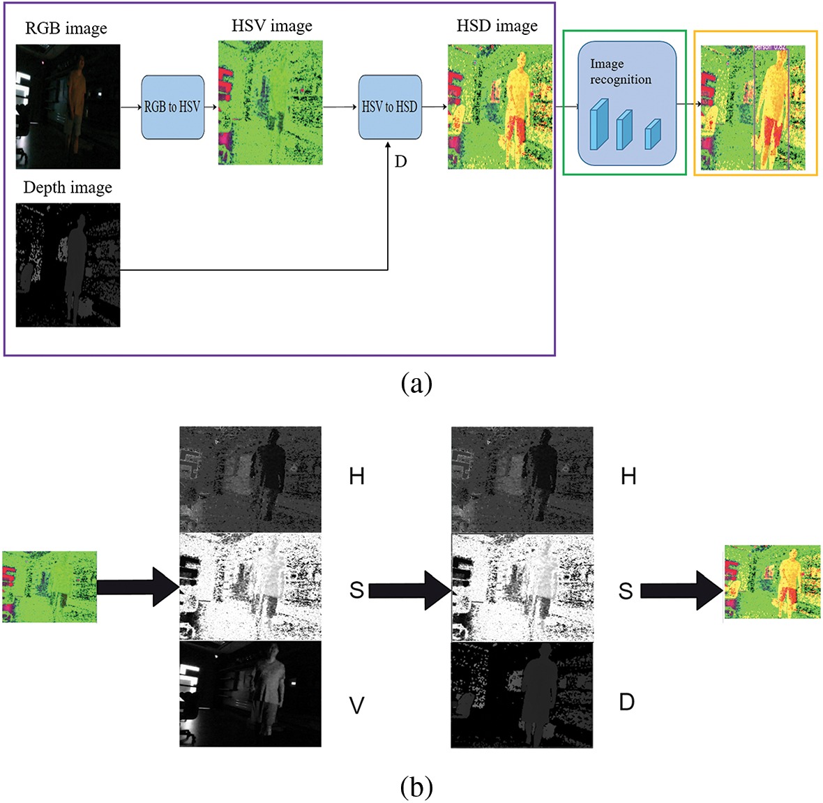
Figure 11: HSD method

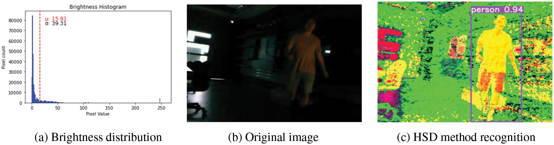
Figure 12: HSD method recognition

4  Results and Discussions

When determining that the imagery is not of low brightness, the RGB image is directly fed into the model designed for normal brightness recognition. The experiment utilized 800 images for training and 250 images with varying brightness levels for validation, each brightness interval containing approximately 50 images. The input image size was set to 512 × 512, and the final training consisted of 300 epochs. Each training iteration had a batch size of 8, with the total training time being approximately 3 h. The hardware setup for the experiment involved a ROG Zephyrus G14 (2022) equipped with an AMD Ryzen 5900HS CPU, 32 GB of memory, and an NVIDIA GeForce RTX 3060 Laptop GPU. The software environment utilized ANACONDA3 with Python version 3.9.1 and YOLOv4 was implemented using PyTorch version 1.12.1 for object recognition. Due to the large size of the dataset used in this experiment, deep learning was chosen over machine learning methods. Fig. 13a illustrates the distribution of the average brightness of images, with an average brightness of 69.65 and a standard deviation of 55.40. Fig. 13b displays the recognition outcome under normal brightness, achieving a recognition rate of 0.97 for the “person” category. The primary focus of this study was on low brightness images, so the following sections discuss the experimental results for each method under different brightness levels individually and then compare the different methods.

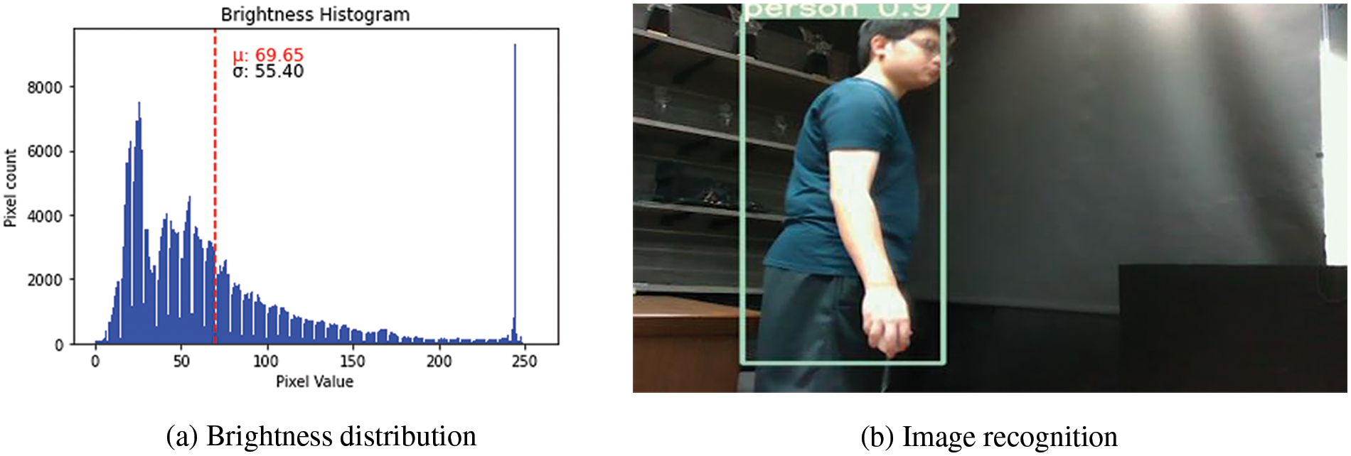
Figure 13: Normal brightness recognition

4.1 SD Method Results

The SD method involves using k-means clustering to segment the depth image, further optimizing the segmentation results through an eight-connected algorithm, and mapping the result onto the RGB image to achieve background removal. During the training process, two different types of images were used for training: Original images and segmented images. Similarly, during recognition, a distinction was made between using original images or segmented images for identification. The recognition was also categorized based on brightness intervals, with approximately 50 images in each brightness interval, divided into ranges of 25~20, 19~15, 14~10, and 9~5 for experimentation. The experiment was conducted in four ways as shown in Table 1: Training on original image/recognition on original image, training on original image/recognition on segmented image, training on segmented image/recognition on original image, and training on segmented image/recognition on segmented image, respectively.

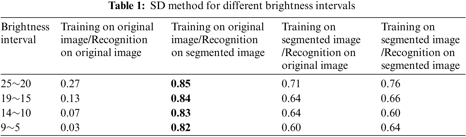
The experimental results indicate that training on original images and recognizing segmented images yields better performance, with most recognition above 0.82. When using segmented images for recognition, removing the background helps reduce noise and interference, allowing the detection process to focus on the target object. Training on segmented images and recognizing original images, while emphasizing the features of the target object during training, introduces background noise interference in the original images during detection, leading to a decrease in recognition accuracy. Training on segmented images and recognizing segmented images may result in information loss during the segmentation process, leading to insufficient features for detection.

4.2 HDV and HSD Method Results

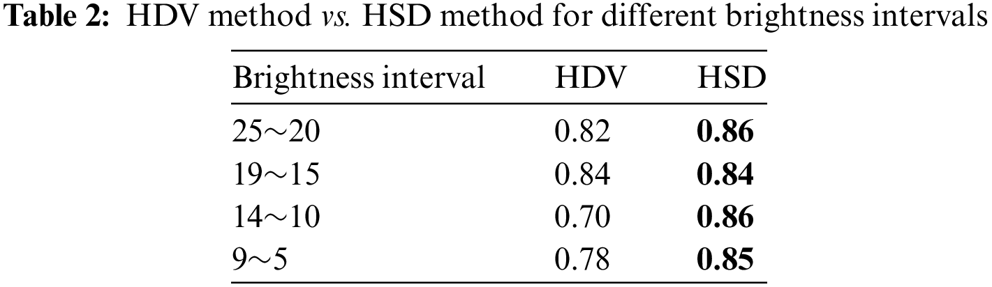
This section directly compares the recognition results of the HDV and HSD methods under different brightness levels, as summarized in Table 2. HDV and HSD both combine RGB and depth images, but it is observed that HSD outperforms HDV. However, to meet the input requirements of the YOLOv4 model, which requires three channels, HDV incorporates depth information by sacrificing some information from the RGB image leading to an increase in misjudgments. On the other hand, HSD adjusts brightness through depth information while preserving the original colors and saturation from RGB. By enhancing the image based on brightness using depth information, HSD achieves a higher recognition rate of over 0.84. The experiment results show that HDV has lower recognition rate when the average brightness of the image goes down to below 14, hitting a low of 0.70.

4.3 Comparison of Three Methods

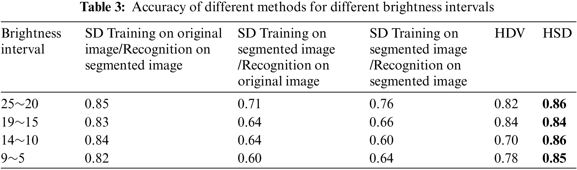
For SD method, the experiment subdivided image segmentation into four modes. The recognition rate of training on original images for recognition on original images is too low and is not included in the comparison here. The other three modes are training on original images for the recognition of segmented images, training on segmented images for the recognition of original images, and training on segmented images for the recognition of segmented images. When experimenting with these three methods, the best results were obtained with training on original images for recognition of segmented images. The HDV method involves converting RGB images to HSV images, losing some information about the S channel, and inserting depth information D to form HDV images. The HSD method similarly converts RGB images to HSV images and enhances the images by replacing the original brightness values V with depth information D.

Table 3 compares various recognition methods in the experiment. In the experimental results, the best performance for the 20–24 brightness interval was achieved by HSD. In other intervals, the HSD image recognition method had a slightly higher average recognition rate, and the results between training on original images for recognition on segmented images and the HSD image recognition method were similar, around 0.82~0.84. However, the recognition rate of HSD remains the highest, maintaining above 0.84, surpassing the training on original images for recognizing segmented objects. Moreover, the HSD method is simple and does not require depth classification of objects, achieving excellent recognition rates directly.

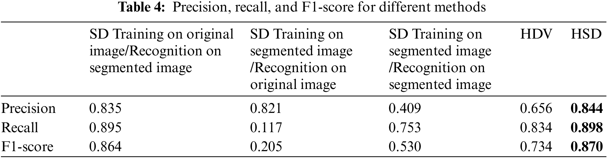
To assess the effectiveness of the experimental model, we begin by defining a confusion matrix consisting of four key elements: True Positives (TP), False Positives (FP), True Negatives (TN), and False Negatives (FN). TP indicates the number of samples correctly identified as “positive,” while FP represents the count of samples incorrectly labeled as “positive.” TN signifies the number of samples correctly classified as “negative,” and FN indicates the instances mistakenly labeled as “negative.” Subsequently, we compute precision using Eq. (7), which measures result relevancy; recall using Eq. (8), quantifying the number of truly relevant results retrieved; and F1-score using Eq. (9), which represents the harmonic mean of precision and recall scores. A higher F1-score indicates a more effective classifier. The experimental findings are summarized in Table 4. Analysis of the table reveals that HSD attains the highest precision, recall, and F1-score, indicating its superiority in both quality and quantity compared to the alternative methods. Specifically, the HSD model demonstrates superior performance by simultaneously achieving the highest accuracy, precision, recall, and F1-score from the results of Tables 3 and 4.

Precision=TPTP+FP(7)

Recall=TPTP+FN(8)

F1 score=21/Precision+1/Recall(9)

5  Conclusions

This study utilizes the Intel Realsense L515 camera to capture RGB and depth images. Through image processing and artificial intelligence training, it successfully recognizes low-light nighttime images with a brightness below 25. The research presents three methods for nighttime image recognition. The SD method involves image segmentation using depth information, achieved through depth k-means classification and connectivity. It separates the background to train and recognize segmented images. Within the brightness interval of 5 to 25, it achieves a recognition rate of 0.82 or higher. The HDV method transforms RGB images into HSV images and replaces the information in the S channel with depth information, resulting in a 3-channel image, HDV. Employing the YOLOv4 object recognition system, the HDV method achieves a recognition rate of 0.70 or higher within the brightness interval of 5 to 25. The HSD method transforms RGB images into HSV images and replaces the information in the V channel with depth information, forming a 3-channel image, HSD. Through the YOLOv4 object recognition system, the HSD method attains a recognition rate of 0.84 or higher. The research findings suggest that the HSD method outperforms the depth information segmentation method, and the depth information segmentation method surpasses the HDV method. The HSD method facilitates a swift and convenient low-light object recognition system, suitable for nighttime surveillance systems or nighttime road safety systems. Future research will implement the proposed method in a mobile robot for nighttime surveillance systems.

Acknowledgement: The authors appreciate LeAnn Eyerman for her hard work and effort in helping as an English editorial reviewer.

Funding Statement: This research was supported by the National Science and Technology Council of Taiwan under Grant NSTC 112-2221-E-130-005.

Author Contributions: S.-Y. Chiang is the corresponding author who conceived the study, contributed to the investigation, development, and coordination, and wrote the original draft preparation. T.-Y. Lin experimented, analyzed data, and processed machine learning in the study. All authors reviewed the results and approved the final version of the manuscript.

Availability of Data and Materials: The data that support the findings of this study are available from the corresponding author, SYC, upon reasonable request.

Conflicts of Interest: The authors declare they have no conflicts of interest to report regarding the present study.

References

1. S. Ren, K. He, R. Girshick, and J. Sun, “Faster R-CNN: Towards real-time object detection with region proposal networks,” IEEE Trans. Pattern Anal. Mach, vol. 39, no. 6, pp. 1137–1149, 2016. doi: 10.1109/TPAMI.2016.2577031. [Google Scholar] [PubMed] [CrossRef]

2. A. Bochkovskiy, C. Y. Wang, and H. Y. M. Liao, “YOLOv4: Optimal speed and accuracy of object detection,” 2020. doi: 10.48550/arXiv.2004.10934. [Google Scholar] [CrossRef]

3. W. Liu et al., “SSD: Single shot multibox detector,” in ECCV 2016: 14th Euro. Conf., Amsterdam, The Netherlands, Oct. 11–14, 2016, pp. 21–37. [Google Scholar]

4. J. Deng, W. Dong, R. Socher, L. Li, K. Li and L. Fei-Fei, “ImageNet: A large-scale hierarchical image database,” in 2009 IEEE CVPR, Miami, FL, USA, 2009, pp. 248–255. doi: 10.1109/CVPR.2009.5206848. [Google Scholar] [CrossRef]

5. T. -Y. Lin et al., “Microsoft COCO: Common objects in context,” in ECCV 2014: 13th Eur. Conf., Zurich, Switzerland, Sep. 6–12, 2014, pp. 740–755. doi: 10.48550/arXiv.1405.0312. [Google Scholar] [CrossRef]

6. X. Dai et al., “Near infrared nighttime road pedestrians recognition based on convolutional neural network,” Infrared Phys. & Tech., vol. 97, pp. 25–32, 2019. doi: 10.1016/j.infrared.2018.11.028. [Google Scholar] [CrossRef]

7. S. M. Pizer et al., “Adaptive histogram equalization and its variations,” Comput. Gr. Image Process., vol. 39, no. 3, pp. 355–368, 1987. doi: 10.1016/S0734-189X(87)80186-X. [Google Scholar] [CrossRef]

8. E. H. Land and J. J. McCann, “Lightness and retinex theory,” J. Opt. Soc. Am., vol. 61, no. 1, pp. 1–11, 1971. doi: 10.1364/JOSA.61.000001. [Google Scholar] [PubMed] [CrossRef]

9. C. Wei, W. Wang, W. Yang, and J. Liu, “Deep retinex decomposition for low-light enhancement,” 2018. doi: 10.48550/arXiv.1808.04560. [Google Scholar] [CrossRef]

10. M. Li, J. Liu, W. Yang, X. Sun, and Z. Guo, “Structure-revealing low-light image enhancement via robust retinex model,” IEEE Trans. on Image Process., vol. 27, no. 6, pp. 2828–2841, 2018. doi: 10.1109/TIP.2018.2810539. [Google Scholar] [PubMed] [CrossRef]

11. X. Guo, Y. Li, and H. Ling, “LIME: Low-light image enhancement via illumination map estimation,” IEEE Trans. on Image Process., vol. 26, no. 2, pp. 982–993, 2016. doi: 10.1109/TIP.2016.2639450. [Google Scholar] [PubMed] [CrossRef]

12. Y. Xiao, A. Jiang, J. Ye, and M. W. Wang, “Making of night vision: Object detection under low-illumination,” IEEE Access, vol. 8, pp. 123075–123086, 2020. doi: 10.1109/ACCESS.2020.3007610. [Google Scholar] [CrossRef]

13. X. Tan, K. Xu, Y. Cao, Y. Zhang, L. Ma and R. W. H. Lau, “Night-time scene parsing with a large real dataset,” IEEE Trans. on Image Process., vol. 30, pp. 9085–9098, 2021. doi: 10.1109/TIP.2021.3122004. [Google Scholar] [PubMed] [CrossRef]

14. T. L. Chia, P. J. Liu, and P. S. Huang, “All-day object detection and recognition for blind zones of vehicles using deep learning,” Int. J. Pattern Recognit. Artif. Intell., vol. 38, no. 1, pp. 2350035, 2023. doi: 10.1142/S0218001423500350. [Google Scholar] [CrossRef]

15. I. Goodfellow et al., “Generative adversarial nets,” in Adv. Neural Inf. Process. Syst., vol. 27, 2014, pp. 27. [Google Scholar]

16. H. Lee, M. Ra, and W. Y. Kim, “Nighttime data augmentation using GAN for improving blind-spot detection,” IEEE Access, vol. 8, pp. 48049–48059, 2020. doi: 10.1109/ACCESS.2020.2979239. [Google Scholar] [CrossRef]

17. J. Y. Zhu, T. Park, P. Isola, and A. A. Efros, “Unpaired image-to-image translation using cycle-consistent adversarial networks,” in Proc. IEEE ICCV, 2017, pp. 2223–2232. doi: 10.48550/arXiv.1703.10593. [Google Scholar] [CrossRef]

18. H. K. I. S. Lakmal and M. B. Dissanayake, “Illuminating the roads: Night-to-day image translation for improved visibility at night,” in Proc. Int. Conf. APAN, 2023, pp. 13–26. [Google Scholar]

19. X. Cheng, J. Zhou, J. Song, and X. Zhao, “A highway traffic image enhancement algorithm based on improved GAN in complex weather conditions,” IEEE Trans. Intell. Transp. Syst., vol. 24, no. 8, pp. 8716–8726, Aug. 2023. doi: 10.1109/TITS.2023.3258063. [Google Scholar] [CrossRef]

20. J. Canny, “A computational approach to edge detection,” IEEE Trans. Pattern Anal. Mach. Intel., vol. PAMI-8, no. 6, pp. 679–698, 1986. doi: 10.1109/TPAMI.1986.4767851. [Google Scholar] [CrossRef]

21. J. M. Prewitt, “Object enhancement and extraction,” Pict. Process. Psychopict., vol. 10, no. 1, pp. 15–19, 1970. [Google Scholar]

22. D. Marr and E. Hildreth, “Theory of edge detection,” in Proc. Roy. Soc. London. Ser. B. Biol. Sci., vol. 207, no. 1167, pp. 187–217, 1980. doi: 10.1098/rspb.1980.0020. [Google Scholar] [PubMed] [CrossRef]

23. M. Ester, H. P. Kriegel, J. Sander, and X. Xu, “A density-based algorithm for discovering clusters in large spatial databases with noise,” in Proc. 2nd Int. Conf. KDD, vol. 96, 1996, pp. 226–231. [Google Scholar]

24. J. MacQueen, “Some methods for classification and analysis of multivariate observations,” in Proc. Fifth Berkeley Symp. Math. Stat. Prob., vol. 1, 1967, pp. 281–297. [Google Scholar]

25. N. Ali, A. Z. Ijaz, R. H. Ali, Z. Ul Abideen, and A. Bais, “Scene parsing using fully convolutional network for semantic segmentation,” in 2023 IEEE CCECE, pp. 180–185, 2023. doi: 10.1109/CCECE58730.2023.10288934. [Google Scholar] [CrossRef]

26. Z. Xie et al., “Boosting night-time scene parsing with learnable frequency,” IEEE Trans. on Image Process., vol. 32, pp. 2386–2398, 2023. doi: 10.1109/TIP.2023.3267044. [Google Scholar] [PubMed] [CrossRef]

27. K. Roszyk, M. R. Nowicki, and P. Skrzypczyński, “Adopting the YOLOv4 architecture for low-latency multispectral pedestrian detection in autonomous driving,” Sens., vol. 22, no. 3, pp. 1082, 2022. doi: 10.3390/s22031082. [Google Scholar] [PubMed] [CrossRef]