Hyperspectral Image Based Interpretable Feature Clustering Algorithm

1  Introduction

Objects possess distinct attributes. Information across various dimensions can be acquired through different detectors. Analyzing the differences and consistencies among targets is of paramount importance. A representative technology in information acquisition is imaging hyperspectral technology, applicable in search and rescue, target identification, and more. It encompasses imaging and spectral detection, enabling spatial feature imaging of targets. Additionally, it allows for continuous spectral coverage by dispersing each spatial pixel into multiple narrow bands, forming a three-dimensional data block [1]. The contained image information reflects external quality characteristics such as size, shape, and defects of the samples. Since different components absorb spectra differently, images at certain wavelengths can significantly highlight specific defects. Spectral information thoroughly represents the internal physical structure and chemical composition differences among samples. These characteristics bestow unique advantages upon hyperspectral imaging technology in detection applications [2].

Leveraging the advantages of hyperspectral imagery, target feature clustering focuses on feature extraction and rapid computation. In feature extraction, the principal aim is to minimize intra-class differences while maximizing inter-class distinctions. Clustering extracts features by considering intra-class variances. Notable algorithms include spatial local similarity [3], Hyperspectral hybrid method [4], Support Vector Machines (SVM) [5], Fuzzy C-Means (FCM) [6], spectral-spatial relations [7], signal response correlation [8], and low rank [9] approaches. Heuristic models underpin clustering philosophies [10]. Classification, conversely, extracts features based on inter-class differences, with representative algorithms encompassing multi-dimensional classifiers [11], texture features [12], K-means [13], multi-scale kernel clustering [14], and graph theory [15]. The emergence of deep learning has introduced new paradigms in feature extraction by establishing mappings between information and semantics, utilizing band similarities to construct networks [16], Deep spatial-spectral subspace [17] approaches, multi-scale models [18], and structural subspaces [19]. These algorithms, rooted in the spatial and spectral relationships of hyperspectral data, model various dimensions to achieve feature extraction. While traditional clustering and classification algorithms are straightforward, significant enhancements in their effectiveness are challenging to achieve. Deep learning-based algorithms, which construct image-semantic relationships, have demonstrated effectiveness across multiple domains. However, features are less interpretable, and substantial annotated samples are required for learning.

In terms of rapid computation, research predominantly focuses on process optimization and network structure. Regarding process optimization, notable algorithms include the development of computational models [20] based on multi-sensor imaging characteristics, downsampling based on band continuity [21], and the construction of anchor graphs for swift feature extraction calculations. In the realm of network structure, advancements involve the graphics processing unit [22], LiteDepthwiseNet [23], attention mechanisms [24], semi-supervised networks [25], and spectral-spatial convolution [26]. These algorithms, primarily serial in nature, facilitate rapid computation of hyperspectral imagery. However, they exhibit certain limitations when applied to diverse tasks.

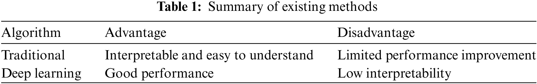
In summary, current algorithms for hyperspectral imagery are mainly divided into those based on traditional features and deep learning (Table 1). Algorithms grounded in traditional features are highly interpretable, predominantly extracting texture and energy-based features. Yet, they lack robustness and significant performance enhancements when dealing with highly variable imagery. Deep learning-based algorithms, which establish image-semantic relationships, exhibit strong robustness following extensive learning but suffer from poor interpretability. The primary challenges faced by both traditional and deep learning algorithms include: 1) High data redundancy, complicating the extraction of representative features; 2) Indistinct intra-class similarities and inter-class differences, making clustering challenging; 3) Prevalent use of serial processing, leading to low efficiency.

Addressing the aforementioned issues, this paper introduces innovative aspects as follows:

•   From a visual perception standpoint, a color-based mapping model is established, presenting interpretable characteristic bands to reduce data dimensions

•   By integrating fuzzy clustering with kernel clustering, a multi-dimensional clustering algorithm is proposed.

•   Inspired by cellular membrane conduction, a tissue-type membrane computing framework is constructed; this facilitates the collaborative computation of optimal cluster centers by all cells within a mapping space, achieving parallel computation.

The paper is structured into four sections. The Section 2 discusses the methodology, encompassing the construction of an interpretable color mapping model, the multi-dimensional clustering algorithm, and the tissue-type membrane computing framework. The Section 3 presents experimental results and analysis, describing the data used for experiments and the computational platform, comparing the proposed algorithm with current mainstream algorithms to validate its effectiveness. The Section 4 concludes the paper, summarizing the strengths and weaknesses of the algorithm and suggesting directions for future research.

2  Algorithm

Hyperspectral imagery is distinguished by its spectral resolution, endowing it with the capability to detect the attributes of terrestrial targets. Compared to panchromatic and multispectral data, hyperspectral data encompasses nearly continuous spectral information of the Earth’s surface. Through spectral reflectance reconstruction, hyperspectral imagery can obtain nearly continuous spectral reflectance curves of the Earth’s surface, thereby enhancing the capability to identify surface cover. Hyperspectral data can detect substances with diagnostic spectral absorption features; it can accurately distinguish between types of vegetation cover, road surface materials, etc. The methods for classifying and identifying terrain features are diverse and flexible, making quantitative or semi-quantitative classification and identification of terrain features feasible. In hyperspectral imagery, it is possible to estimate the status parameters of various terrestrial objects, thus improving the precision and reliability of high-quantitative remote sensing analysis.

This paper proposes a clustering algorithm for interpretable features based on hyperspectral imagery, as illustrated in Fig. 1. Initially, leveraging the Gestalt principles of vision and simulating the RGB imaging principle, a database of ten colors is constructed. The relationship between color and the database is established, endowing the clustering features with interpretability. Subsequently, by analyzing the correlation between frames, a fuzzy kernel clustering algorithm is constructed to reduce the sensitivity to initial cluster centers. An interaction mechanism between local optima and global optima is established to avoid entrapment in local optima. Finally, to enhance computational capabilities, a tissue P system is designed, inspired by cellular structures, to achieve parallel computation.

Figure 1: Algorithm flow chart

2.1 Interpretable Band Selection Algorithm

The Gestalt principles posit that human perception of objects results from the combined action of the eye and brain [27], adhering to the following principles: 1) Figure and ground: Within a given configuration, some objects emerge as figures while others recede to serve as the background. 2) Proximity and continuity: Parts that are close or adjacent to each other tend to form a whole. 3) Completeness and closure: Perceptual impressions tend to present themselves in the most complete form possible, depending on the environment. 4) Similarity: If parts are equidistant but differ in color, those of the same color naturally coalesce into a whole. 5) Invariance: According to homomorphism, Gestalts, being isomorphic with the stimulus patterns, can undergo extensive changes without losing their inherent characteristics. In imaging principles, the RGB imagery mode aligns with visual principles and is readily accepted by humans.

Drawing on Gestalt theory, an interpretable band selection algorithm is proposed. Hyperspectral imagery, represented by discrete points, is considered as continuously varying based on the principles of proximity and continuity. The band selection model is constructed using the principles of similarity and invariance. By extracting three bands from the hyperspectral image sequence to form a pseudo-color image, the process simulates visual perception, enhancing the consistency within the same category and the differences between distinct categories, and presents these variations in color.

Considering the sensitivity of visual perception, RGB colors are categorized into ten types. The differences between the three channels (C1, C2, C3 and the standard colors (Ra, Ga, Ba) are calculated using Euclidean distance. When ξ is minimized, the three channel values are normalized to the corresponding standard colors.

ξ=mina(|C1−Ra|+|C2−Ga|+|C3−Ba|)(1)

This approach enables the pseudo-color mapping of different bands, as shown in Fig. 2, intuitively displaying the differences in targets within specific spectral bands. This band selection method aligns with the principles of visual perception and is interpretable by presenting the information in the form of colors.

Figure 2: Color mapping model

2.2 Multi-Dimensional Clustering Algorithm

Hyperspectral imagery can be perceived as a data cube, where frames exhibit strong correlations and similarities. To extract representative bands for image clustering, the spatial relationships within images are considered. Direct application of kernel-based distance algorithms fails to fully exploit the characteristics of imagery. Moreover, clustering is relatively clear in most image areas but challenging around boundaries and transition zones. Therefore, a fuzzy clustering algorithm is adopted, focusing on ambiguous regions. Inspired by kernel clustering, data is transformed to a higher dimension for analysis to uncover more representative features, highlighting intra-class similarities and inter-class differences.

Fuzzy clustering analysis clusters objective entities based on their features and similarities, establishing fuzzy similarity relations [28]. This approach is aligned with the principles of visual perception, focusing on the transition zones between targets to extract features. Let the pixels contained in an image form a dataset M = {x1, x2,…, xn}, where n is the pixel resolution.

Assuming the clustering algorithm partitions M into k clusters C, in fuzzy clustering, each pixel has its membership degree, denoted as uij for the membership degree of the jth pixel in the ith cluster. Fuzzy partitioning satisfies the condition:

{0<∑j=1nμij<n,i=1,2…k∑i=1nμij=1j=1,2…n,∑i=1k∑j=1nμij=nuij∈[0,1](2)

The objective function for classical fuzzy C-means clustering is defined as:

JC=min∑j=1n∑i=1k(μij)m‖xj−zi‖2(3)

where zi represents the center of the ith cluster, and xj represents the jth data point in the dataset.

The concept of kernel clustering involves mapping data to a high-dimensional feature space, thereby enabling the clustering of data of any shape [29]. The process is as follows: The dataset X is mapped to a high-dimensional feature space, represented as φ: Rd→ H, xi → φ(xi), where xi = [ xi,1, xi,2,…xi,d]T. A kernel function is introduced to measure the distance between two points:

D(φ(xi),φ(xj))=||φ(xi)−φ(xj)||2=k(xi,xi)−2k(xi,xj)+k(xj,xj)(4)

where k(xi, xj) denotes the kernel function. Common kernel functions include linear, polynomial, Gaussian, Laplacian, and Sigmoid kernels.

On this basis, the optimal clustering centers are sought. The objective function is constructed:

J=min∑i=1k∑j=1n(uij)mD(φ(xj),φ(zi))(5)

The integration of fuzzy clustering with kernel clustering algorithms is pursued; pixels are mapped to a high-dimensional feature space, and an objective function is designed to find the optimal cluster centers:

J′=min{∑i=1k∑j=1n(μij)mD(φ(xj),φ(zi))+α∑i=1k∑j=1nD(φ(x^j),φ(zi))}(6)

μij=[D(φ(xj),φ(zi))+α(D(φ(x^j),φ(zi)))]11−m∑i=1k[1−D(φ(xj),φ(zi))+α(1−D(φ(x^j),φ(zi)))]11−m(7)

where x^j represents the average grayscale value in the neighborhood of the (jth) pixel. Thus, the problem of pixel clustering in images is transformed into an optimization problem of the objective function.

2.3 Framework of Tissue P System

Given the high dimensionality and computational demands of hyperspectral imagery, scholars, inspired by cellular transmission structures, introduced P systems [30]. A typical P system comprises skin membranes, basic membranes, and non-basic membranes. Based on the transmission process, these can be classified into cellular, neural, numerical, and tissue types. The cellular system operates with cells as independent computational units, as illustrated in Fig. 3a. It achieves optimal results through the promotion and sharing between different cells. The neural system represents neurons with each node, simulating the mechanism of pulse neurons through synaptic connections, with pulse signals stored in neurons. The numerical system substitutes nested membrane structures of linguistic characters with numerical variables. The tissue system, depicted in Fig. 3b, can be seen as a network of processors, facilitating information exchange and sharing among basic membranes through objects.

Figure 3: Typical Psystem block diagram

Given the processor network characteristics of tissue systems, they are well-suited for image clustering. Consequently, a tissue P system was designed as the computational framework. Within this system structure, there are q cells, each containing m objects, with each object representing a set of candidate cluster centers. Assuming the dataset to be clustered is X, divided into k clusters C, each object, representing a set of candidate cluster centers, is denoted as Z = {φ(z1), φ(z2), …, φ(zk)}. This leads to the relationship between the original space, feature space, and P system, as shown in Fig. 4.

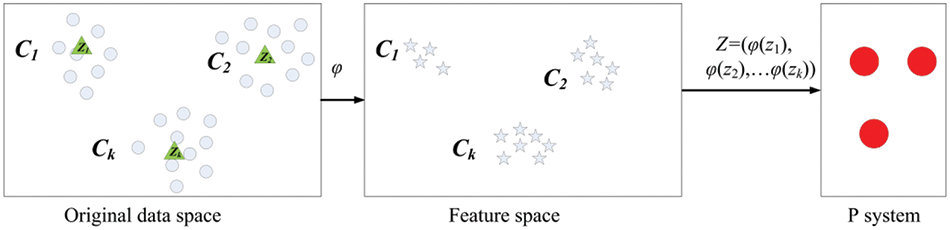
Figure 4: P system object representation

The tissue P system, with its network membrane structure, situates each cell within a common public environment. Through evolution and operation rules, the optimal cluster centers are stored, defined as:

M=(O1,O2,…On,R,Q,i0)(8)

where On represents the nth cell, R the evolution rules, Q the operation rules, and i0 the output result after transmission.

In the process of identifying optimal cluster centers, each object represents a set of candidate cluster centers, denoted as Z = {z1, z2,..., zk}, where k is the number of cluster centers. The data is mapped to a high-dimensional space through the mapping function φ( ), represented as O = {φ(z1), φ(z2), …, φ(zk)}.

Building on the P system framework and incorporating a velocity and displacement model, the model is enhanced as follows:

{Vi=w1Oi+w2(pi−Oi)+w2(OB−local−Oi)+w3(OB−ground−Oi)Oi′=Oi+Vi(9)

where wn represents the weight parameter. OB-local denotes the optimal object within the OB-ground cell, and OB-ground represents the optimal object under global conditions. The rule change between the environment and cells adopts the (i, OB-local/λ, OB-ground) rule, comparing the effects of OB-local and OB-ground to select the optimal outcome.

3  Experiment Result and Analysis

This research selected a database composed of 300 sets of 16-bit hyperspectral data. Half of these datasets were generated using hyperspectral simulation software based on extensive data collected by various devices in earlier phases, while the other half consisted of actual data collected by developed hyperspectral equipment, spanning the visible to near-infrared spectral range. The software environment was Win7. Professionals conducted pixel-level calibration of ground objects within the data, serving as the gold standard, with a training-to-testing data ratio of 1:1.

3.1 Experimental Data

A spectral image dataset was constructed, with representative images displayed in Fig. 5. DATA 1 and 2, the simulated data, have a spatial resolution of 1024 × 768 and 200 spectral bands. DATA 3 and 4, actual shot data, have a spatial resolution of 1392 × 1395 and 256 spectral bands. The spectral curves of typical ground objects are shown in Fig. 6. The spectral curve of the sky differs significantly from those of other ground objects, while the difference between the spectral curves of sand and grassland is less pronounced. Analyzing the full spectral range does not highlight the differences between them. Thus, a clustering algorithm for interpretable features based on hyperspectral imagery was proposed to emphasize the distinctions between different ground objects.

Figure 5: Data display

Figure 6: Spectral curve of a typical feature

3.2 Evaluation Metrics and Parameter Selection

Accuracy (ACC), Compactness (CP), Adjusted Rand Index (ARI) and Kappa coefficient were introduced as metrics to evaluate the outcomes from various dimensions. ACC calculates the proportion of pixels correctly clustered within the image:

ACC=∑i=1kniN(10)

where N denotes the total number of pixels in the image and ni represents the number of correctly classified pixels. ACC is directly proportional to performance.

CP measures the compactness of cluster centers:

CP=1K∑k=1K∑xi∈Ωi‖xi−wi‖|Ωi|(11)

where wi denotes the center of the ith cluster. CP is directly proportional to performance.

ARI assesses the degree of agreement in data classification:

ARI=RI−E[RI]max(RI)−EI,RI=a+bC2n(12)

where C represents the labeled class information, K the clustering information, a represents the number of elements in the same category in both C and K, and B represents the number of elements in different categories of K in month C. C2n indicates the total number of elements in the dataset.

The Kappa coefficient is used as a consistency check metric, where N represents the total number of samples, r the number of rows in the confusion matrix, xij and the value of the element in the ith row and jth column of the confusion matrix. xi+ denotes the sum of the ith row, and x+i the sum of the ith column of the confusion matrix.

Kappa=N∑i=1rxii−∑i=1r(xi+×x+i)N2−∑i=1r(xi+×x+i)(13)

AOM, AVM, AUM, and CM measure segmentation outcomes from different dimensions.

AOM=S∩GS∪G,AVM=S−GS,AUM=G−SG,CM=13{AOM+(1−AVM)+(1−AUM)}(14)

where S represents the manually annotated results and G the algorithm-annotated results. AOM and CM are directly proportional to segmentation performance, whereas AVM and AUM are inversely proportional to segmentation performance.

The kernel function serves as a parameter in this algorithm. Representative linear, polynomial, and Gaussian kernels were selected for statistical analysis. The linear kernel function (Linear) is denoted as:

k(xi,xj)=xi⋅xj(15)

The polynomial kernel function (Poly) is expressed as:

k(xi,xj)=(xi⋅xj+1)a(16)

The Gaussian kernel function (Gauss) is represented as:

k(xi,xj)=exp⁡(−‖xi−xj‖22σ2)(17)

The effect of different kernel clustering is shown in Table 2, where V represents the corresponding index value and E represents the index improvement rate:

Exy=Vx−VyVy×100%(18)

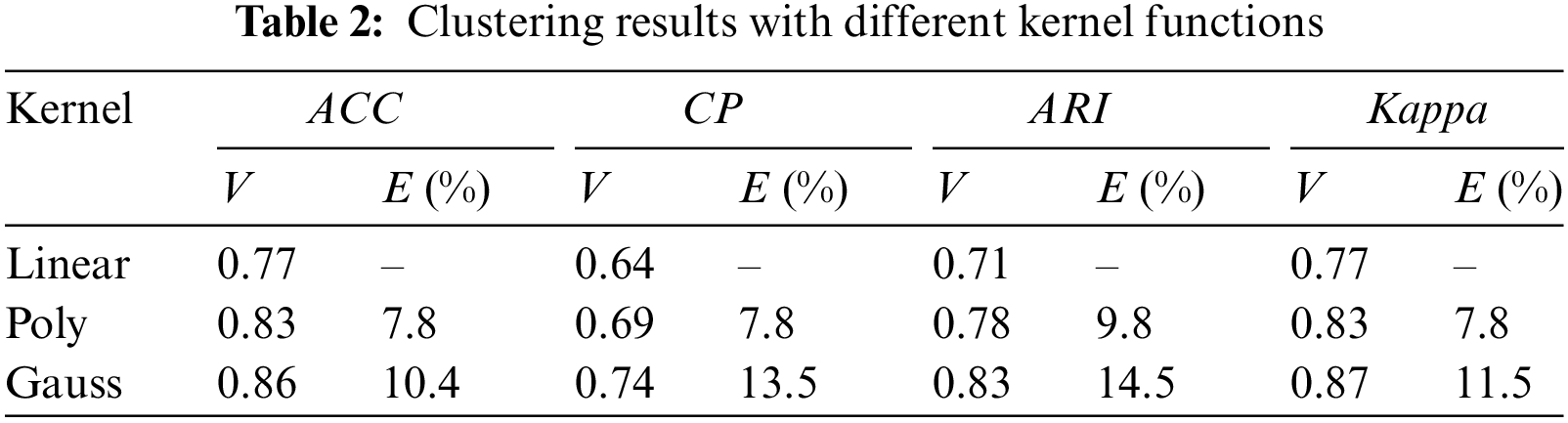
where we take the index result of Linear kernel as the benchmark, then x takes the index of Linear kernel, and y is the index of Poly and Gauss, respectively. It can be seen the Gaussian kernel achieves the best results. EGauss, Linear is 10.4. For a visual demonstration, a hyperspectral image was selected, with its pseudo-color image displayed in Fig. 7a. The result using the linear kernel is shown in Fig. 7b. The simplicity of the kernel function does not effectively suppress noise, leading to suboptimal results. The polynomial kernel result, illustrated in Fig. 7c, employs a curve to filter the image, somewhat mitigating noise. It improves efficiency by first calculating polynomial terms in higher dimensions before inner product. The Gaussian kernel result is depicted in Fig. 7d. The Gaussian kernel, with its stronger mapping capability, yields the best outcome. Additionally, with the Gaussian kernel function, k(xi, xi) = 1, leading to a simplified objective function:

Figure 7: Images of clustering results with different kernel functions. (a) Pseudo-color image corresponding to hyperspectral imagery; (b) clustering result using linear kernel; (c) clustering result using polynomial kernel; (d) clustering result using Gaussian kernel

J′=min{∑i=1k∑j=1n(μij)m(1−K(xj−zi))+∑i=1k∑j=1n(μij)m(1−K(x^j−zi))}(19)

Thereby it significantly enhances computational efficiency.

Hyperspectral images from different bands were selected to form simulated RGB images, as shown in Fig. 8. Analysis leads to the following conclusions: 1) The real RGB images appear dark due to the evening shooting scene, making it challenging to accurately distinguish ground objects. 2) The representational capacity of a single spectral band is limited. 3) Combinations of different bands reveal variations, thereby highlighting the characteristics of various ground objects. In summary, the construction of image combinations from different bands, based on Gestalt theory and mapping colors to ten categories, uses representative bands to emphasize the features of different ground objects, achieving a display that aligns with human visual perception.

Figure 8: Combined mapping images of different spectral bands

3.3 Comparison of Clustering Algorithms

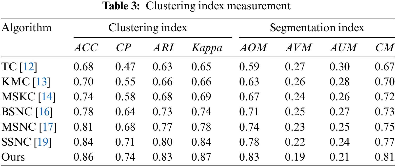
To validate the effectiveness of the proposed hyperspectral clustering algorithm, traditional Texture Clustering (TC) [12], K-Means Clustering (KMC) [13], Multi-scale Kernel Clustering (MSKC) [14], and deep learning-based approaches such as Band Similarity Network Clustering (BSNC) [16], Multi-Scale Network Clustering (BSNC) [18] and Structural Subspace Network Clustering (BSNC) [19] were selected for comparison with this research’s algorithm. The evaluation focused on clustering and segmentation performance. Quantitative metrics, as presented in Table 3, indicate that all algorithms achieved clustering. Methods based on traditional features showed lower performance. Deep learning-based algorithms exhibited higher effectiveness, with the algorithm proposed in this research outperforming the others. The TC algorithm clusters based on texture features formed by boundaries between substances, achieving certain effectiveness when the boundaries in the captured scenes are distinct. However, variability in material responses across different spectral bands may lead to inaccurate boundary extraction. The KMC algorithm constructs clustering models based on the similarity of spectral curves of similar materials. The method demonstrates effectiveness for hyperspectral images with simple scenes. However, as scene complexity increases, clustering becomes disordered. The MSKC algorithm constructs kernel functions at multiple scales to capture information from different dimensions, enhancing clustering performance beyond the first two algorithms. The BSNC algorithm, by learning from a large amount of statistical hyperspectral data, establishes a mapping between bands and semantics, achieving clustering. The MSNC algorithm integrates multi-scale information into a deep network, offering stronger representational capabilities and robustness compared to MSKC. The SSNC algorithm models from a spatial perspective to analyze intra-class similarities and inter-class differences, yielding favorable results. The algorithm proposed in this research, by constructing a model from the perspectives of fuzzy and kernel clustering, builds a membrane computing framework on the premise of ensuring clustering accuracy, achieving rapid clustering with optimal results.

ROC curves were calculated for four datasets, with the algorithm’s performance visually displayed in Fig. 9. Datasets 1 and 2 consist of simulated data with lower resolution, minimal noise, and strong spectral regularity. Datasets 3 and 4 comprise real collected data with higher resolution and noise, particularly in images captured at night. Dataset 1 primarily contains land and grassland, with its ROC curve shown in Fig. 9a. The clear boundaries between different ground objects allowed all algorithms to achieve favorable results. Dataset 2, containing land and grassland, presents a more complex scene than Dataset 1. The oblique angle of hyperspectral data acquisition results in a blurred transition zone between land and sand in the upper part of the image, as shown in Fig. 9b, slightly reducing algorithm performance. However, the performance difference between traditional and deep learning-based algorithms is minimal. With real collected data, a more significant performance decline is observed. Dataset 3 includes sky, vegetation, cars, and land, with its ROC curve shown in Fig. 9c. Adequate lighting and distinct image features contribute to better algorithm performance, despite the complexity introduced by noise and tree branches. Dataset 4, captured in the evening within the same environment as Dataset 3, has its ROC curve depicted in Fig. 9d. Distinguishing different ground objects in nighttime hyperspectral imagery is visually challenging, leading to a marked decline in traditional algorithm performance. The algorithm proposed in this research, by selecting bands and analyzing the combination effects of different spectral bands from an interpretable and visually intuitive perspective, still achieves favorable results, demonstrating the effectiveness of the proposed method.

Figure 9: Algorithm clustering effect display

4  Conclusions

Hyperspectral imagery, encompassing spatial and spectral information, can intuitively display the spatial and material information of ground objects, holding vast potential for theoretical research and practical applications. Addressing the challenges of large data volumes and redundancy in hyperspectral data, which complicate clustering, an interpretable feature clustering algorithm for hyperspectral imagery was proposed. The innovations of this research include: 1) Building a color mapping model based on visual principles and introducing an interpretable band selection model to reduce data dimensions. 2) Integrating fuzzy and kernel clustering to thoroughly explore image features, achieving minimal intra-class differences and significant inter-class variations. 3) Proposing a tissue P computing framework to facilitate rapid computation.

However, the research encountered some issues requiring further investigation: 1) The real data collected for experiments originated from a single model of spectrometer, without considering the variability in data obtained by different spectrometer models. 2) The current research’s data was limited to the infrared and near-infrared spectral ranges; further validation is needed to determine whether the algorithm can be extended to other spectral ranges such as long-wave and ultraviolet.

Acknowledgement: The authors also grate fully acknowledge the helpful comments and suggestions of the reviewers, which have improved the presentation.

Funding Statement: This work is supported by Yulin Science and Technology Bureau production Project “Research on Smart Agricultural Product Traceability System” (No. CXY-2022-64); Light of West China (No. XAB2022YN10); The China Postdoctoral Science Foundation (No. 2023M740760); Shaanxi Province Key Research and Development Plan (No. 2024SF-YBXM-678).

Author Contributions: Yaming Kang and Peishun Ye performed the experiments. Yuxiu Bai and Shi Qiu analyzed the data. All authors conceived and designed research, and contributed to the interpretation of the data and drafting the work.

Availability of Data and Materials: The data used to support the findings of this study are available from the corresponding author upon request.

Conflicts of Interest: The authors declare no conflict of interest.

References

1. J. Zhang et al., “A survey on computational spectral reconstruction methods from RGB to hyperspectral imaging,” Sci. Rep., vol. 12, no. 1, pp. 1–17, 2022. doi: 10.1038/s41598-022-16223-1. [Google Scholar] [PubMed] [CrossRef]

2. U. Bhatti et al., “Deep learning-based trees disease recognition and classification using hyperspectral data,” Comput. Mater. Contin., vol. 77, no. 1, pp. 681–697, 2023. doi: 10.32604/cmc.2023.037958. [Google Scholar] [CrossRef]

3. H. Yu et al., “Global spatial and local spectral similarity-based manifold learning group sparse representation for hyperspectral imagery classification,” IEEE Trans. Geosci. Remote Sens., vol. 58, no. 5, pp. 3043–3056, 2019. doi: 10.1109/TGRS.2019.2947032. [Google Scholar] [CrossRef]

4. S. Ghaderizadeh, D. Abbasi-Moghadam, A. Sharifi, N. Zhao, and A. Tariq, “Hyperspectral image classification using a hybrid 3D-2D convolutional neural networks,” IEEE J. Sel. Top. Appl. Earth Obs. Remote Sens., vol. 14, pp. 7570–7588, 2021. doi: 10.1109/JSTARS.2021.3099118. [Google Scholar] [CrossRef]

5. O. Okwuashi and C. Ndehedehe, “Deep support vector machine for hyperspectral image classification,” Pattern Recognit., vol. 103, no. 4, pp. 107298, 2020. doi: 10.1016/j.patcog.2020.107298. [Google Scholar] [CrossRef]

6. S. Qiu, P. Zhang, X. Tang, Z. Zeng, M. Zhang, and B. Hu, “Sanxingdui cultural relics recognition algorithm based on hyperspectral multi-network fusion,” Comput. Mater. Contin., vol. 77, no. 3, pp. 3783–3800, 2023. doi: 10.32604/cmc.2023.042074. [Google Scholar] [CrossRef]

7. X. Du, X. Zheng, X. Lu, and X. Wang, “Hyperspectral and LiDAR representation with spectral-spatial graph network,” IEEE J. Sel. Top. Appl. Earth Obs. Remote Sens., vol. 16, pp. 9231–9245, 2023. doi: 10.1109/JSTARS.2023.3321776. [Google Scholar] [CrossRef]

8. Y. Chen, S. Ma, X. Chen, and P. Ghamisi, “Hyperspectral data clustering based on density analysis ensemble,” Remote Sens. Lett., vol. 8, no. 2, pp. 194–203, 2017. doi: 10.1080/2150704X.2016.1249295. [Google Scholar] [CrossRef]

9. H. Zhai, H. Zhang, L. Zhang, and P. Li, “Laplacian-regularized low-rank subspace clustering for hyperspectral image band selection,” IEEE Trans. Geosci. Remote Sens., vol. 57, no. 3, pp. 1723–1740, 2018. doi: 10.1109/TGRS.2018.2868796. [Google Scholar] [CrossRef]

10. C. Ding et al., “Hyperspectral image classification promotion using clustering inspired active learning,” Remote Sens., vol. 14, no. 3, pp. 596, 2022. doi: 10.3390/rs14030596. [Google Scholar] [CrossRef]

11. B. Jia and M. Zhang, “Decomposition-based classifier chains for multi-dimensional classification,” IEEE Trans. Artif. Intell., vol. 3, no. 2, pp. 176–191, 2021. doi: 10.1109/TAI.2021.3110935. [Google Scholar] [CrossRef]

12. H. Su, Y. Sheng, P. Du, C. Chen, and K. Liu, “Hyperspectral image classification based on volumetric texture and dimensionality reduction,” Front. Earth Sci., vol. 9, no. 2, pp. 225–236, 2015. doi: 10.1007/s11707-014-0473-4. [Google Scholar] [CrossRef]

13. J. Haut, M. Paoletti, J. Plaza, and A. Plaza, “Cloud implementation of the K-means algorithm for hyperspectral image analysis,” J. Supercomput, vol. 73, no. 1, pp. 514–529, 2017. doi: 10.1007/s11227-016-1896-3. [Google Scholar] [CrossRef]

14. J. Feng, L. Jiao, T. Sun, H. Liu, and X. Zhang, “Multiple kernel learning based on discriminative kernel clustering for hyperspectral band selection,” IEEE Trans. Geosci. Remote Sens., vol. 54, no. 11, pp. 6516–6530, 2016. doi: 10.1109/TGRS.2016.2585961. [Google Scholar] [CrossRef]

15. Y. Cai, Z. Zhang, Z. Cai, X. Liu, X. Jiang and Q. Yan, “Graph convolutional subspace clustering: A robust subspace clustering framework for hyperspectral image,” IEEE Trans. Geosci. Remote Sens., vol. 59, no. 5, pp. 4191–4202, 2020. doi: 10.1109/TGRS.2020.3018135. [Google Scholar] [CrossRef]

16. Q. Wang, F. Zhang, and X. Li, “Optimal clustering framework for hyperspectral band selection,” IEEE Trans. Geosci. Remote Sens., vol. 56, no. 10, pp. 5910–5922, 2018. doi: 10.1109/TGRS.2018.2828161. [Google Scholar] [CrossRef]

17. J. Lei, X. Li, B. Peng, L. Fang, N. Ling, and Q. Huang, “Deep spatial-spectral subspace clustering for hyperspectral image,” IEEE Trans. Circuits Syst. Video Technol., vol. 31, no. 7, pp. 2686–2697, 2020. doi: 10.1109/TCSVT.2020.3027616. [Google Scholar] [CrossRef]

18. S. Polk and J. Murphy, “Multiscale clustering of hyperspectral images through spectral-spatial diffusion geometry,” in 2021 IEEE Int. Geosci. Remote Sens. Symp. IGARSS, Brussels, Belgium, 2021, pp. 4688–4691. [Google Scholar]

19. S. Huang, H. Zhang, and A. Pižurica, “Semisupervised sparse subspace clustering method with a joint sparsity constraint for hyperspectral remote sensing images,” IEEE J. Sel. Top. Appl. Earth Obs. Remote Sens., vol. 12, no. 3, pp. 989–999, 2019. doi: 10.1109/JSTARS.2019.2895508. [Google Scholar] [CrossRef]

20. W. Wang, W. Wang, and H. Liu, “Correlation-guided ensemble clustering for hyperspectral band selection,” Remote Sens., vol. 14, no. 5, pp. 1156, 2022. doi: 10.3390/rs14051156. [Google Scholar] [CrossRef]

21. T. Imbiriba, J. Bermudez, C. Richard, and J. Tourneret, “Band selection in RKHS for fast nonlinear unmixing of hyperspectral images,” in 2015 23rd Eur. Signal Process. Conf. (EUSIPCO), Nice, France, IEEE, 2015, pp. 1651–1655. [Google Scholar]

22. J. Nalepa, “Recent advances in multi-and hyperspectral image analysis,” Sens., vol. 21, no. 18, pp. 6002, 2021. doi: 10.3390/s21186002. [Google Scholar] [PubMed] [CrossRef]

23. B. Cui, X. Dong, Q. Zhan, J. Peng, and W. Sun, “LiteDepthwiseNet: A lightweight network for hyperspectral image classification,” IEEE Trans. Geosci. Remote Sens., vol. 60, pp. 1–15, 2021. doi: 10.1109/TGRS.2021.3062372. [Google Scholar] [CrossRef]

24. S. Qiao, X. Dong, J. Peng, and W. Sun, “LiteSCANet: An efficient lightweight network based on spectral and channel-wise attention for hyperspectral image classification,” IEEE J. Sel. Top. Appl. Earth Obs. Remote Sens., vol. 14, pp. 11655–11668, 2021. doi: 10.1109/JSTARS.2021.3124321. [Google Scholar] [CrossRef]

25. B. Fang, Y. Li, H. Zhang, and J. Chan, “Collaborative learning of lightweight convolutional neural network and deep clustering for hyperspectral image semi-supervised classification with limited training samples,” ISPRS J. Photogramm. Remote Sens., vol. 161, no. 2, pp. 164–178, 2020. doi: 10.1016/j.isprsjprs.2020.01.015. [Google Scholar] [CrossRef]

26. Z. Meng, L. Jiao, M. Liang, and F. Zhao, “A lightweight spectral-spatial convolution module for hyperspectral image classification,” IEEE Geosci. Remote Sens. Lett., vol. 19, pp. 1–5, 2021. doi: 10.1109/LGRS.2021.3069202. [Google Scholar] [CrossRef]

27. S. Qiu, Y. Jin, S. Feng, T. Zhou, and Y. Li, “Dwarfism computer-aided diagnosis algorithm based on multimodal pyradiomics,” Inform. Fusion, vol. 80, no. 1, pp. 137–145, 2022. doi: 10.1016/j.inffus.2021.11.012. [Google Scholar] [CrossRef]

28. G. Liu, Y. Zhang, and A. Wang, “Incorporating adaptive local information into fuzzy clustering for image segmentation,” IEEE Trans. Image Process., vol. 24, no. 11, pp. 3990–4000, 2015. doi: 10.1109/TIP.2015.2456505. [Google Scholar] [PubMed] [CrossRef]

29. A. Elazab, C. Wang, F. Jia, J. Wu, G. Li and Q. Hu, “Segmentation of brain tissues from magnetic resonance images using adaptively regularized kernel-based fuzzy-means clustering,” Comput. Math. Methods Med., vol. 485495, pp. 1–12, 2015. doi: 10.1155/2015/485495. [Google Scholar] [PubMed] [CrossRef]

30. T. Wang et al., “A weighted corrective fuzzy reasoning spiking neural P system for fault diagnosis in power systems with variable topologies,” Eng. Appl. Artif. Intel., vol. 92, no. 8, pp. 103680, 2020. doi: 10.1016/j.engappai.2020.103680. [Google Scholar] [CrossRef]