Blood Pressure Estimation with Phonocardiogram on CNN-Based Approach

1  Introduction

Blood pressure (BP) is a crucial vital sign in the human body, serving as a significant risk indicator for serious health conditions, notably cardiovascular diseases (CVD) and hypertension [1–5]. A reliable, continuous, and non-invasive BP monitoring method could significantly aid healthcare providers in enhancing the prevention, detection, and diagnosis of hypertension and effectively managing related treatment strategies [6–8]. Various factors, including abnormalities in cardiac output, blood vessel wall elasticity, blood volume circulation, peripheral resistance, respiration, and emotional behavior, significantly influence BP [1,9–11]. Given the intricate and dynamic nature of the cardiovascular system, any BP monitoring system should ideally leverage intelligent technology capable of extracting and analyzing significant BP features [8,12–14]. Traditional BP measurement methods [1,15] and the use of handcrafted features for continuous BP monitoring prove to be cumbersome and computationally demanding [3,16–19]. Recent research has explored BP measurement through engineered feature [3]. BP is influenced by numerous physiological and neurological factors, and incorporating feature extraction into a BP estimation model could markedly enhance measurement accuracy [3,20–22]. Phonocardiogram (PCG) signals have emerged as a valuable and non-invasive source of information for the estimation of blood pressure, a vital physiological parameter crucial for monitoring cardiovascular health [1,8,13,23]. PCG signals are acoustic recordings of heart sounds, capturing the mechanical events within the cardiac cycle [20,24,25]. PCG is a commonly used feature for developing BP measurement models, recognized as a valid and well-accepted method for estimating BP [17,20,24]. Nonetheless, methods dependent on hand-engineered face significant limitations [12,18,19,22,26].

The calculation of multiple features simultaneously proves challenging due to individual specific waveforms and the impact of motion artifacts [10,25]. Additionally, extracting desired features is cost intensive and time consuming in real-time monitoring scenarios [27]. Artificial Intelligence (AI), particularly deep learning algorithms within machine learning, emerges as a promising technique for recognizing complex function patterns and emulating the non-linear relationship between non-linear system inputs and outputs. This approach has demonstrated encouraging results in biomedical technologies, including hypertension risk assessment and echocardiography image analysis [2,19]. Deep learning methods hold promise for extracting features from blood pressure (BP) and classifying other physiological signals [28,29]. They can also be applied for BP estimation, offering a potential pathway for continuous and non-invasive BP monitoring [3,24].

However, the type of Convolutional Neural Networks (CNN) that will be used in the experiment, typical CNNs for 1D data, may struggle to effectively handle the spatial changes and variations inherent in the BP signal [24]. This is necessary to ensure accurate BP measurement, considering these limitations. This paper therefore proposes the use of CNN, which is a more advanced and flexible neural network layer structure. It is designed to adjust the sampling position in the feature map. This adaptability allows the model to better handle a wide range of signal formats. It provides a new efficient solution for BP estimation using CNN. We expect it to challenge another method of BP estimation. Previous methods generally struggle to handle diverse and complex BP signal formats [3]. Even some previous studies have talked about using more than one signal and combining it with a CNN to get an estimation. This innovative approach is expected to increase the learning capabilities of the model. This could lead to more accurate, reliable, and efficient blood pressure estimation [12,18,22,26]. The proposed method is likely to contribute significantly to advances in continuous blood pressure monitoring technology. To the best of our knowledge, this is the first instance of employing an end-to-end CNN designed specifically to process raw PCG signals for the purpose of blood pressure estimation. Our pioneering strategy eliminates the necessity for expert-driven feature extraction and selection, markedly streamlining the analytical process. Moreover, our research benefits from an extensive dataset of authentic PCG signals, gathered from 78 participants in a stud. This breakthrough not only improves the accessibility of the model but also broadens its applicability in clinical environments, heralding significant progress in the precision and dependability of non-invasive blood pressure monitoring methods. The introduction of this method stands to revolutionize the management and preliminary detection of coronary artery disease and hypertension.

2  Materials and Methods

2.1 Dataset

For this study, a specialized database was diligently compiled, focusing exclusively on phonocardiogram signals to ensure the robustness and reliability of the proposed blood pressure estimation models [11,25]. The database encompasses PCG signal data from a diverse cohort of participants, spanning various ages, genders, and health conditions. This extensive diversity is pivotal for affirming the effectiveness and reliability of the proposed models across a wide array of individuals, ensuring the models’ broad applicability and generalizability in real-world settings. Fig. 1 is the sample of the PCG signal.

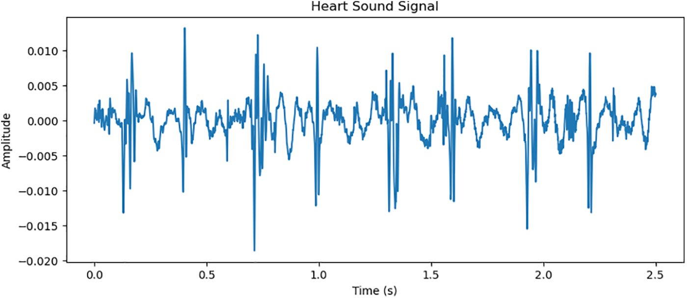
Figure 1: Simultaneous presentation physiological signals PCG of the arterial pressure

Data collection:

The data collection was carried out under strictly controlled conditions to minimize the impact of external variables on the PCG signals and the corresponding BP readings [11]. Participants were comfortably seated in a calm, temperature-regulated environment to ensure consistent and accurate PCG signal recordings. The dataset captured signals within the frequency range of 20–2000 Hz. Sensors were positioned for optimal PCG signal reception on participants. Efforts were made to minimize distractions and noise. We meticulously collected PCG signal data from 78 volunteers, which was considered and approved by the Human Research Ethics Committee Suranaree University of Technology. The research was conducted in accordance with the ethical principles for human research in accordance with the Declaration of Helsinki. Received research ethics certificate number Suranaree University of Technology. The procedure for collecting PCG signal data, along with blood pressure values, is outlined in Fig. 2.

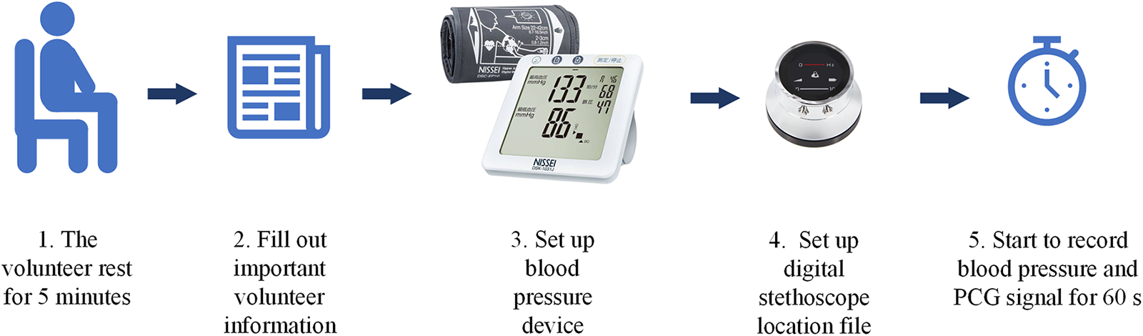
Figure 2: Sequence of recording PCG signal from volunteer

1.   Participants sat comfortably in a calm, temperature-controlled environment for approximately 5 min to ensure consistent and accurate recording of the PCG signal.

2.   Interview basic important information from volunteers, including age, weight, height, and gender.

3.   Prepare the automatic blood pressure monitor. Ready to use a pressure measuring strap (Cuff) to wrap around the upper arm approximately 1–2 inches above the elbow and tie it tightly.

4.   Prepare the digital stethoscope equipment to record signals. and set the signal file name to match the information of each volunteer.

5.   Place the digital stethoscope in the position specified by the attending physician. After that, start the automatic blood pressure monitor and record the PCG signal.

Equipment for data collection:

Blood pressure monitor: In this research, an automatic blood pressure recording device named Blood Pressure Monitor NISSEI DSK-1031 was used.

Digital stethoscope: The ThinkLabs One Digital Stethoscope was employed, featuring a frequency range of 20–2000 Hz.

Fig. 3 shows the new dataset being tested in a hospital. The physician is responsible for overseeing the collection of data from each volunteer. The test was conducted under human research ethics number EC-65-78.

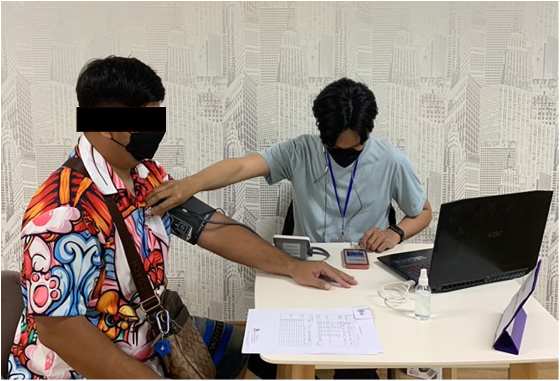
Figure 3: Simultaneous recording of PCG signals and measurement of blood pressure take place concurrently

2.2 PCG Signal Processing

In the preparation of the database for model development and evaluation, a comprehensive data pre-processing and PCG signal processing phase was meticulously conducted. This multifaceted process entailed the meticulous removal of noise and artifacts from the PCG signals, ensuring the presence of pristine and high fidelity signals ideal for feature extraction and subsequent model training [3,24]. Simultaneously, the associated blood pressure readings underwent rigorous verification and validation procedures to validate their accuracy and reliability. Within the PCG signal processing framework, a rigorous pre-processing routine was applied to enhance signal quality, encompassing noise and artifact removal, amplitude normalization for standardization, and segmentation to partition the continuous PCG signals into manageable segments, facilitating further in-depth analysis [5,10].

2.3 Blood Pressure Estimation Methods

2.3.1 1D CNN-Based Method

In the Traditional CNN-based Method, the features from the PCG signals are used as the input to a Convolutional Neural Network for blood pressure estimation [24]. To adapt CNNs for time-dependent applications, modifications are made to exploit their ability to learn hierarchical patterns, now from sequences observed over time. By applies a 1D convolutional neural networks over an input signal composed of several input planes. Such adaptations make CNNs suitable for a wide range of time series, which following in the Eqs. (1) and (2). Let X be the matrix of PCG signals features, the CNN maps these features to an estimated blood pressure using a function by the weights θ of the network:

y[t]=∑i=0k−1x[t+i]⋅w[i]+b(1)

where

y[t] is the value of the output at time step t.

x[t+i] represents the input values at time steps t,t+1,t+2,…,t+k−1.

w[i] represents the convolutional kernel weights at index i.

b is the bias term.

Lout=[Lin+2(p)−1(k−1)−1s+1](2)

Lout is the length of the output sequence.

Lin is the length of the input sequence.

p is the amount of padding added to each side of the input sequence.

k is size of the convolving kernel.

s is stride of the convolution.

The network comprises multiple convolutional layers followed by pooling layers, fully connected layers, and a regression output layer. The convolutional layers apply a set of learnable filters to the input features. Fig. 4 shows a diagram illustrating the envisioned Conv1D model structure, from input into the solving Eq. (2). The overall approach employs a 5-layer CNN and depicts the constituent elements of each CNN layer [30].

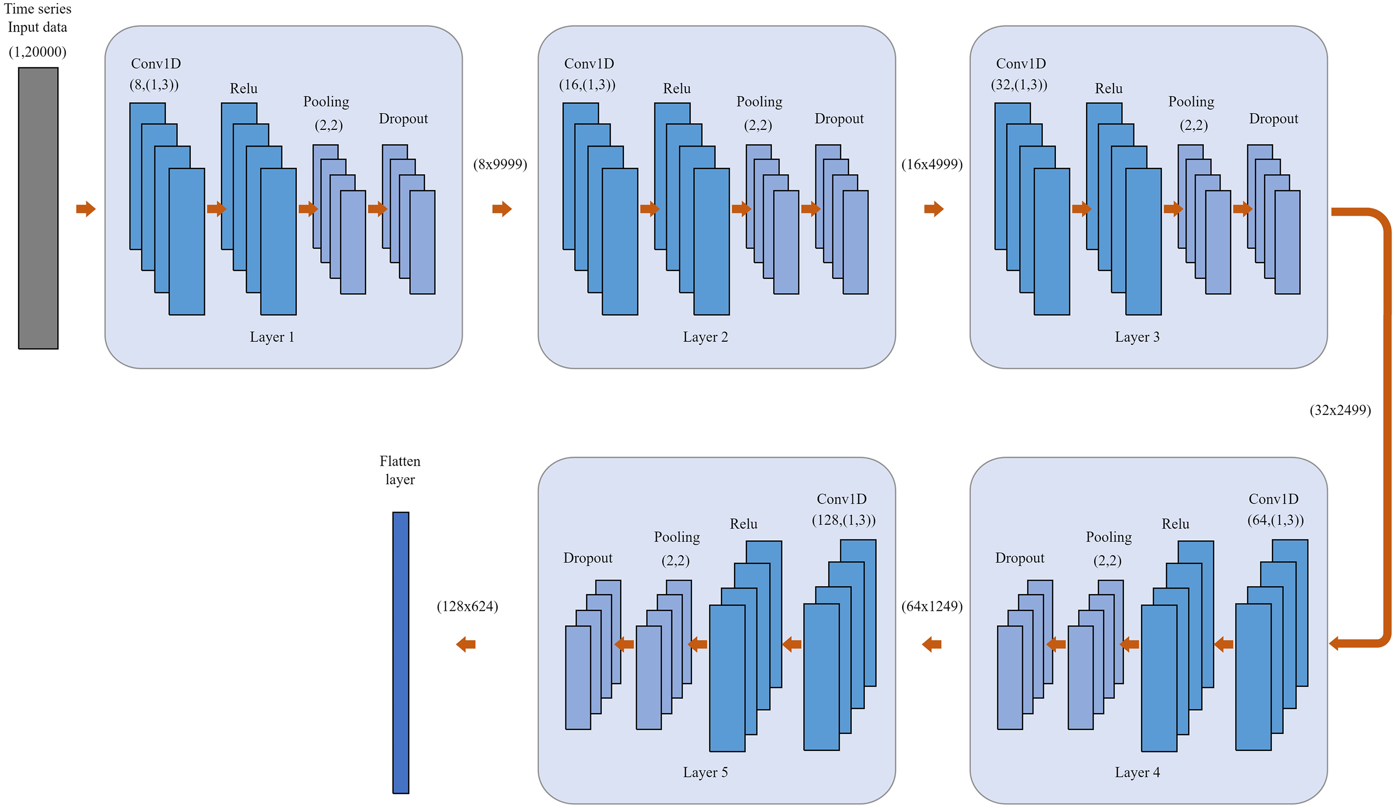
Figure 4: A schematic representation of the proposed Conv1D model architecture. Overall method using 5-layer CNN and shown the component of CNN layer

3  Experimental Setup

3.1 Design Model Training

3.1.1 Dataset Split

In this study, a 3-fold cross-validation approach is employed to ensure the robust evaluation of the models. The entire dataset, encompassing PCG signals and corresponding blood pressure readings, is evenly divided into three folds. In each iteration of the validation process, two folds (approximately 67% of the data) are used for training the model, and the remaining one-fold (approximately 33% of the data) is used for validation [31]. This process is repeated three times, with each fold used for validation exactly once. After the completion of the 3-fold cross-validation, the average performance metrics from each fold are computed to obtain a comprehensive and reliable assessment of the models’ performance. This approach ensures that every data point is used for both training and validation, enhancing the reliability of the model evaluation and ensuring the models’ effectiveness and generalizability across diverse data samples. For final testing and evaluation, a separate test set, which was not involved in the 3-fold cross-validation, is used. This test set in each iteration comprises 1 fold of the total 3 fold shown in Fig. 5 and 2 fold using for training. K-fold cross-validation is utilized to assess the models’ performance on unseen data, providing insights into their real-world applicability and effectiveness in blood pressure estimation from PCG signals. In each iteration, the test performance of each fold after iteration. Result will be taken to the next average performance.

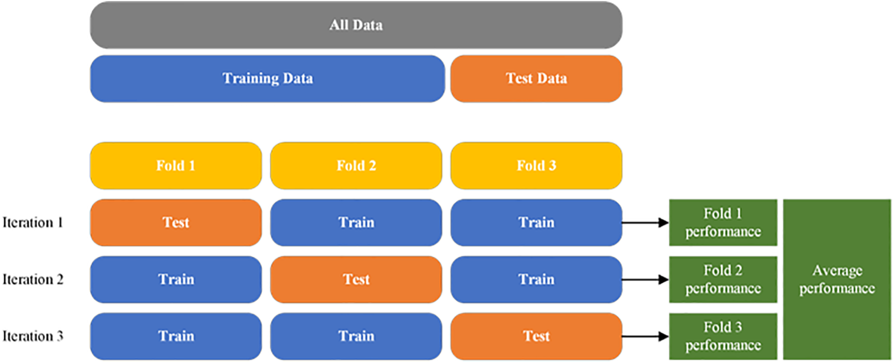
Figure 5: Illustration of the K-fold cross-validation

3.1.2 Data Augmentation

To enhance the balance of the models and mitigate overfitting, data augmentation techniques are employed. These techniques include adding white Gaussian noise, time shifting, and time stretching to the PCG signals. This augmentation enriches the diversity of the training data, enabling the models to learn more generalized and robust features [28].

Additive white Gaussian noise (AWGN): In this technique, white Gaussian noise is introduced into the PCG signals. This noise, following a Gaussian distribution, simulates real-world variations and adds a level of randomness to the signals. By doing so, the models become more resilient to noise in actual data, leading to improved generalization and reduced overfitting.

We have added the adding white Gaussian noise as one of the data augmentation techniques to the text. This technique helps to further diversify the training data and improve the model’s robustness.

3.1.3 Model Architecture

Architecture the CNN-based models are constructed with multiple layers, including convolutional layers, pooling layers, and fully connected layers. The CNN-based model incorporates convolutional layers that adaptively adjust the sampling locations in the feature map in Fig. 6, enhancing the model’s ability to capture complex patterns in the PCG signals.

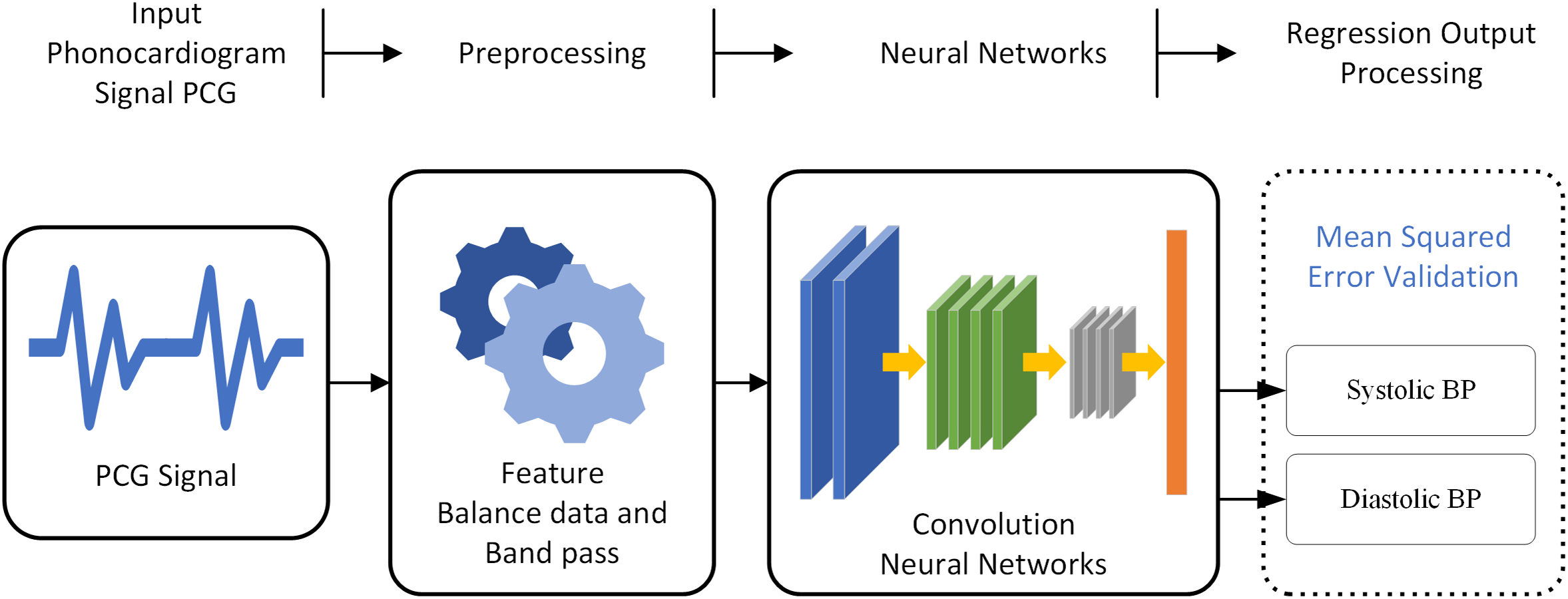
Figure 6: A block diagram depicting the overall system of estimate BP from the PCG signal

3.1.4 Loss Function

The Mean Squared Error (MSE) loss function is used to train the models. It calculates the average squared differences between the estimated and actual blood pressure values, guiding the models to minimize this error during the training process [28,31].

MSE=1n∑i=1n(xi−xi∧)2(3)

where (xi) and (xi∧) are the actual and estimated blood pressure values, respectively, and n is the number of observations. The Mean Squared Error (MSE) loss function is used to measure the average squared difference between predicted values and actual values in a regression task.

The MSE loss measures the discrepancy between predicted values (xi) and actual values (xi∧) for each data point in the dataset. The goal is to minimize this loss during the training process to make predicted values as close as possible to the ground truth values.

3.1.5 Optimizer

The Adam optimizer is employed for training the models. It adaptively adjusts the learning rate during training, providing efficient and effective optimization.

3.1.6 Training Process

In the training process, machine learning or deep learning models are iteratively optimized to achieve optimal performance on a given task. This section outlines the key aspects of the training process.

1. Epoch-Based Training:

The training process is organized into epochs, where each epoch represents a complete pass through the entire training dataset. This approach allows the model to iteratively learn and improve from the data. The training process will repeat 2000 times, each time adjusting the model’s parameters to reduce the error in predictions. In Fig. 7, through experimentation, we observed that our model’s loss function started stabilized around 1750 epochs, with marginal improvements thereafter. Extending the training to 2000 epochs allowed us to confirm that the model reached in learning, and for training with the newly PCG dataset. thereby ensuring that we had fully captured the learning potential of the newly data without prematurely halting the process.

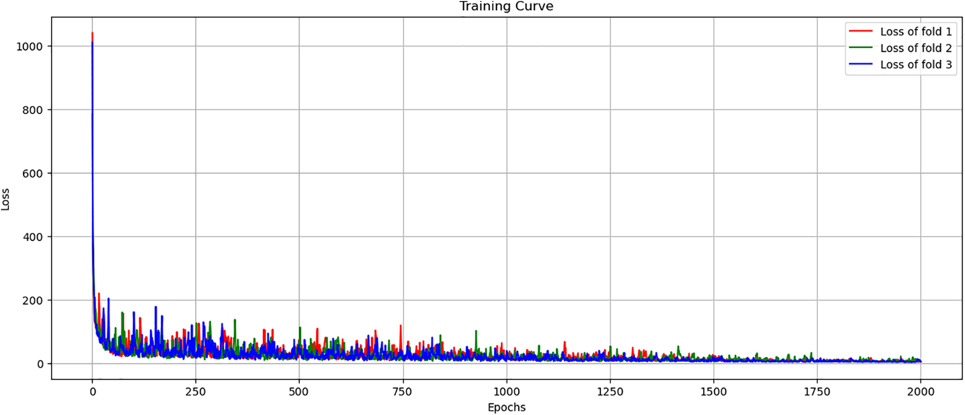
Figure 7: Training loss curve across 3-fold cross-validation

2. Optimize Model Performance:

The Adam optimizer is used to adjust and improve model parameters based on the calculated gradients. Adam is chosen for its effectiveness in handling varying data scales and its adaptive approach to adjusting the learning rate, which is essential for converging to optimal solutions efficiently.

3. Loss Function:

The Mean Squared Error Loss (MSE) function is used to measure the difference between the model’s predictions and the actual values. MSE is a common choice for regression problems as it penalizes larger errors more severely, encouraging the model to focus on reducing these larger discrepancies.

3.1.7 Hyperparameter Tuning

Various hyperparameters Including learning rate and batch size. This process involved employing a systematic method to select the most effective conditions based on their performance outcomes in initial experiments. These conditions were then iteratively applied to refine subsequent experiments. To explore the conditions of various parameters systematically and identify the configuration that provides the best model performance from this new recording dataset.

1.   CNN layer and pooling: The design of our CNN model’s architecture, specifically the configuration of its convolutional and pooling layers, is informed by the guidelines established in reference [28]. Initially, the model is structured to include three convolutional layers, a foundational setup aimed at capturing a broad range of features from the input data. Following each convolutional layer, a max pooling layer is integrated, serving as a critical component for reducing dimensionality, enhancing computational efficiency, and ensuring the model’s focus on the most salient features. This initial configuration, chosen as our test’s starting condition.

2.   Learning rate: The learning rate is a critical hyperparameter in the training of neural networks. In this section, the learning rates to be tuned are 0.01, 0.001, and 0.0001. The learning rate influences how much the model’s weights are adjusted during training. A higher rate can lead to faster convergence but might overshoot the minimum, while a lower rate ensures more precise updates but can slow down the training process. The goal is to find an optimal learning rate that balances convergence speed and accuracy.

3.   Batch size: Batch size is another key hyperparameter, and the sizes being experimented with are 256, 128, 64, 32, and 16 [30]. The batch size determines the number of training examples used in one iteration of model updates. Larger batch sizes offer more stable gradient estimates but require more memory and computational power. Conversely, smaller batch sizes can lead to faster convergence and can also introduce beneficial noise, aiding generalization. The ideal batch size would efficiently utilize computational resources while maintaining good model performance.

3.1.8 Model Evaluation

Upon completion of training, the models are evaluated on the test set to assess their performance using the metrics outlined in the Performance Criteria section. The results from this evaluation provide insights into the models’ effectiveness in blood pressure estimation from PCG signals and inform potential refinements and enhancements for further model development.

3.2 Performance Criteria

In evaluating the performance of the proposed CNN-based learning regression model for blood pressure estimation, several key metrics are employed to ensure a comprehensive assessment. These metrics provide a quantitative measure of the model’s accuracy, reliability, and overall effectiveness in estimating blood pressure from PCG signals. Below are the detailed explanations and equations for each performance criterion used in this study:

•   Mean Absolute Error (MAE): This metric calculates the average absolute errors between the estimated and the actual blood pressure values. It provides a straightforward measure of the model’s estimation error. A lower MAE value indicates better performance of the model.

MAE=1n∑i=1n|yi−yi∧|(4)

•   Standard Deviation (STD): The standard deviation of the errors measures the dispersion of the errors from the mean error. A lower STD indicates that the errors are closely clustered around the mean, suggesting consistent model performance.

STD=1n∑i=1n(yi−yi∧)2(5)

Each of these performance criteria plays a crucial role in thoroughly evaluating the effectiveness of the proposed model, ensuring its reliability and accuracy in real-world blood pressure estimation tasks. The comprehensive assessment allows for the identification and addressing of any potential limitations or areas of improvement, contributing to the continual enhancement of the model’s performance in blood pressure estimation from PCG signals.

4  Results and Discussion

4.1 Results Based on Our Proposed Method

The model proposed a Mean Absolute Error (MAE) of systolic and diastolic pressure estimation. These results are expected to approach the acceptable margin of error within the Association for the Advancement of Medical Instrumentation (AAMI) standard. This emphasizes the clinical applicability of the mode.

4.1.1 Comparison with Method

In this subsection, we compare the performance of our proposed method with that of several well-known systems. As mentioned in the introduction section, some systems may not be included due to differences in the experimental models employed in database-based approaches. Here, we present a comparison of experimental results to align with the conditions of our experiment. As a result, we include the results of select known systems for the purpose of adjusting continuous testing and comparing them with the methods we have tested. Table 1 presents the overall performance, including the Mean Absolute Error (MAE) and Standard Deviation (STD), for both the training and testing phases of each network. It can be observed that the CNN with three CNN layers and three hidden layers has a linear layer for test the new dataset. This network utilizes the PCG signals recorded from 78 volunteers in the dataset.

The MAE SBP value of 32.46 mmHg represents the average systolic blood pressure in the STD dataset. An SBP of 24.97 mmHg indicates a degree of variability or dispersion of SBP values. A higher standard deviation indicates a measurement range. A broader SBP MAE DBP value of 19.81 mmHg represents the average diastolic blood pressure in the STD dataset. DBP of 15.39 mmHg represents the variability in DBP measurements. MBP of 26.13 mmHg represents the average of both SBP and DBP. And provide insight into overall blood pressure. In summary Table 1, it is a test of this dataset when imported into the estimation process with the CNN technique to see if the newly recorded data can produce a preliminary estimation or not. As shown in the table, Using this new dataset can be used in the basic CNN system, but the tolerances of the test results are not acceptable. The next step was to further improve the test by rebalancing the dataset to balance the values that could be estimated. and increase the chances of the machine learning to learn from an increased dataset

In our examination of the newly acquired PCG signal data, we identified significant fragmentation with an underrepresentation of higher blood pressure readings. To rectify this imbalance and improve the dataset’s efficacy for model training, we implemented Additive White Gaussian Noise (AWGN) as a deliberate method to enrich the dataset with a wider spectrum of blood pressure readings. This enrichment strategy was aimed at bolstering the dataset with additional data points across a broader blood pressure range, thereby facilitating a more comprehensive model training.

The impact of this data augmentation is graphically depicted in Fig. 8. Here, kernel density estimates provide a stark comparison between the distribution of the unmodified dataset and that which has been enhanced with AWGN. The density plots demonstrate how the application of AWGN successfully expands the representation of higher blood pressure values, mitigating the initial disproportionality and fostering a more balanced dataset for the development of our model. Table 2 shows the MAE with AWGN method.

Figure 8: Kernel density estimates for the distribution of blood pressure data comparing without AWGN to those with AWGN

The presence of AWGN clearly has a significant effect on blood pressure estimation when comparing the two rows. Table 2 shows that when testing the same model, The finding that the MAE was much lower when the data were balanced across different blood pressure values. This is due to the assumption that if there is an increase in the distribution of information in training, It will make learning work better because there are a number of datasets that are known along with the values used in training. When testing the results, it was found that adding a more balanced number of trainings sessions to the dataset resulted in weaker estimation results. To evaluate the CNN model design, we performed tests and compared the results. Specifically, investigating the variation in extracting PCG signal features under different numbers of CNN layers, the results are shown in Table 3.

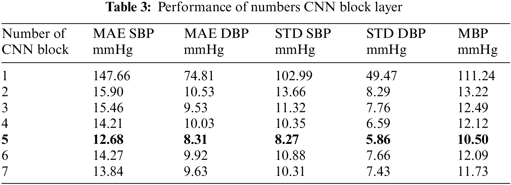
The results of the experimental table where different modifications of the CNN layers are presented and compared. Among these modifications. The experiment yielded significantly low error values. It had a pressure error of 12.68 mmHg for the upper pressure and 8.31 mmHg for the lower pressure. As shown in Table 3. The results in Table 3 reveal a trend in the performance of a CNN model with varying numbers of convolutional blocks, as measured by MAE for SBP, DBP blood pressure, and their STD, along with MBP. A notable observation is the decrease in MAE for both SBP and DBP as the number of CNN blocks increases from 1 to 5, indicating improved model accuracy. However, this improvement plateaus beyond five layers, suggesting an optimal number of layers for this specific application. The standard deviations also follow a similar trend, decreasing with an increasing number of layers, indicating more consistent model predictions. This analysis reflects the efficiency of deep learning models in capturing complex patterns in data, with a balance between model complexity and performance. From the experimental results in the Table 3, there are 7 layers of CNN presented, because in the test adding layers at 8, 9, 10, the results obtained from the estimation were under-fitting of estimation. And this continued to happen as more layers of the CNN were added, allowing us to continue testing other types of parameterizations.

The next phase involves examining Table 4, which is to analyze the impact of different numbers of linear layers, following the model with 5 CNN layers. This investigation aims to assess how various linear layer configurations influence the model’s precision and reliability in blood pressure measurement. Such an analysis is crucial for determining the most effective number and configuration of linear layers to optimize the model’s performance for the specific application at hand.

In our analysis of Table 4, we focused on the MAE performance of models with different numbers of linear layers for estimating blood pressure. Several noteworthy trends have emerged. The key factor under investigation is the number of linear layers within the model architecture.

Firstly, we observe a clear relationship between the number of linear layers and MAE values. As the number of linear layers increases from 1 to 8, a consistent impact is observed on both systolic blood pressure (SBP) and diastolic blood pressure (DBP) MAE. For SBP MAE, the highest value of 19.05 mmHg is associated with a model featuring 1 linear layer. However, as the number of linear layers progressively increases, SBP MAE consistently decreases. The most accurate SBP estimation, with an MAE of 11.68 mmHg, is achieved when employing models with 6 linear layers. A parallel trend is observed for DBP MAE, with the highest MAE of 74.73 mmHg linked to 1 linear layer, while the lowest DBP MAE of 7.88 mmHg is attained with 6 linear layers.

Secondly, the analysis extends to the STD of SBP and DBP MAE. These STD values exhibit a consistent pattern mirroring the behavior of MAE. As the number of linear layers increases, STD values decrease, reflecting a reduction in variability. Models with 1 linear layer produce the highest STD values, signifying greater variability in MAE. Conversely, models with 6 linear layers yield the lowest STD values, indicating reduced variability in MAE.

Lastly, the Mean Blood Pressure (MBP) values align with the trends observed for SBP and DBP MAE. The highest MBP MAE is associated with 1 linear layer, while the lowest MBP MAE is achieved when employing models with 6 linear layers.

In summary, the analysis highlights the important role of selecting the appropriate number of linear layers within the model architecture. For accurate blood pressure estimation, The model with 6 linear layers outperformed the other models. Consistently, showing lower MAE and lower STD in MAE, these findings highlight the importance of optimizing the number of linear layers to effectively increase the accuracy of blood pressure estimation. From the experimental results in Table 4, there are 8 linear layers presented because in the test plus the 9th layer, the results obtained from the estimation caused underfitting to the estimation. And this continues to happen as more linear layers are added. This leads us to continue testing other types of parameterizations.

The next step involves testing by adjusting the values in specific learning areas. Scale the data to be fed into the learning section and compile the learning rate values in Table 5.

The analysis of the results presented in Table 5, which investigates the MAE performance of models across different batch sizes and learning rates, offers valuable insights into the influence of these hyperparameters on the accuracy of blood pressure estimation.

Considering the impact of learning rate on MAE, the results show that learning rate selection plays an important role in accurate blood pressure estimation. A higher learning rate (0.01) tends to result in lower MAE values, indicating increased accuracy in estimating blood pressure. On the contrary The lowest learning rate (0.0001) often leads to higher MAE values, highlighting the importance of an appropriate learning rate in achieving model convergence and accuracy. Table 5, which examines the MAE performance across different batch sizes and learning rates, reveals several trends. Smaller batch sizes, particularly 16, demonstrate lower MAE values in many cases, suggesting better model performance. This can be attributed to smaller batch sizes offering more frequent updates and potentially better generalization. The interaction between batch size and learning rate also appears significant; for instance, a batch size of 16 with a learning rate of 0.01 shows notably lower MAE values across most table, indicating an optimal combination for this specific model and dataset. This suggests that both the batch size and learning rate play crucial roles in model accuracy and should be carefully tuned to achieve optimal performance.

Table 5 is observed with a batch size of 16 and a learning rate of 0.01. This combination yields the lowest Mean Absolute Error (MAE) values across the board: SBP (10.69 mmHg), DBP (6.89 mmHg), STD SBP (7.23 mmHg), STD DBP (5.22 mmHg), and MBP (8.79 mmHg). This indicates that for this model and dataset, a smaller batch size combined with a moderately high learning rate optimizes performance, leading to more accurate blood pressure predictions with lower variability.

Fig. 9 shows is a scatter plot illustrating the correlation between blood pressure values predicted by our model and the actual blood pressure measurements. The plot showcases how closely our model’s estimates align with the true values. This visual representation demonstrates the effectiveness of our proposed in estimating blood pressure.

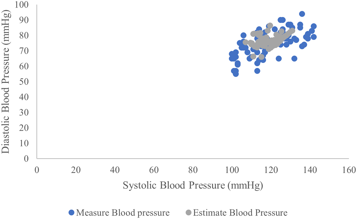
Figure 9: Scatter plot both actual and estimated blood pressure values by the proposed model

4.1.2 Systolic Blood Pressure Estimation

To estimate systolic blood pressure model performed. It has an MAE 10.69 mmHg, Fig. 10a, and a standard deviation is 7.23 mmHg, indicating that the model estimates can provide an approximation to the real data. This indicates linear relationship between the estimated and actual systolic blood pressure values. These findings reinforce the model’s feasibility for estimating systolic blood pressure. This points to the potential usefulness of the PCG signal feature in this context, and it is clear from the picture that the estimated vs. actual values tend to be similar.

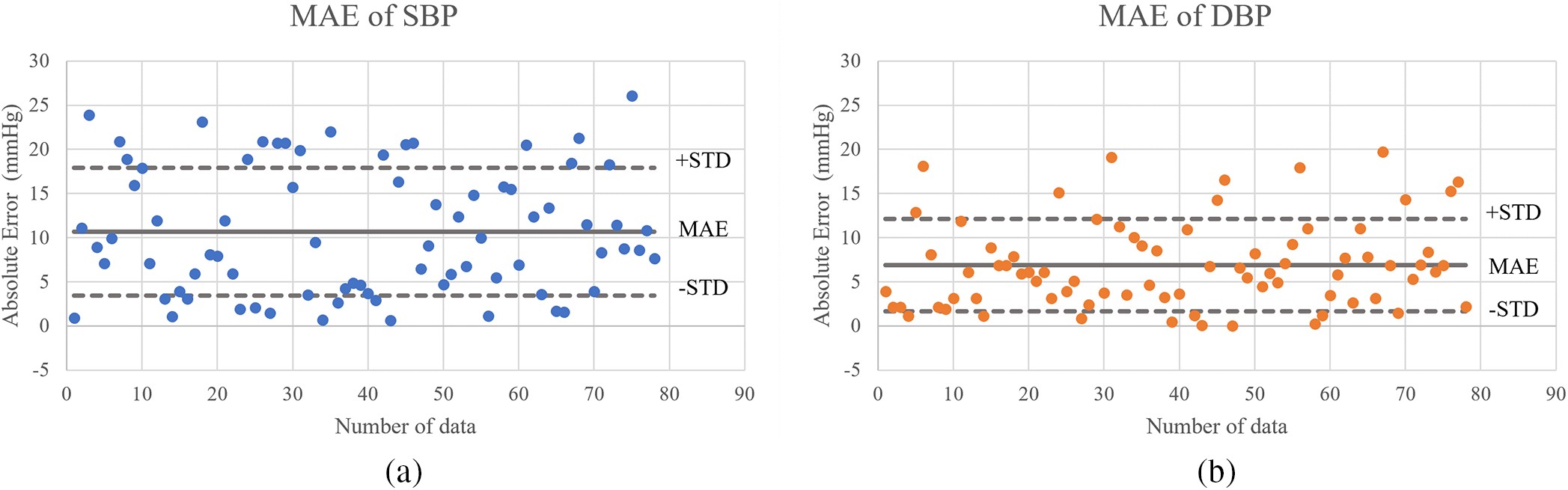
Figure 10: Scatter plot of the algorithm for (a) systolic BP estimation and (b) diastolic BP estimation

4.1.3 Diastolic Blood Pressure Estimation

In terms of diastolic blood pressure estimation, it comes to estimating diastolic blood pressure model performed. With a mean absolute error of 6.89 mmHg. This indicates a lower error rate compared to systolic blood pressure values. The standard deviation of the error was recorded as 5.22 mmHg. Fig. 10b visually shows that the model’s estimates correspond closely to the real data. These findings also confirm the model’s consistent performance in estimating systolic and diastolic blood pressure.

4.2 Comparison of the Results with the Related Works

Table 6 presents a comprehensive comparative analysis of the performance of PCG-based blood pressure estimation using the proposed CNN approach in this study, along with recent related works from the literature. The evaluation is based on key metrics, including Mean Absolute Error and Standard Deviation [3,32], for both systolic blood pressure and diastolic blood pressure. Table 6 presents a comprehensive comparison of CNN-based PCG methods for blood pressure estimation. This work is detailed alongside other contemporary studies such as the use of PCG signals with traditional machine learning techniques and artificial neural networks. Work using dual signals, namely PCG and PPG for blood pressure estimation This demonstrates the diversity of approaches within the field. This table includes the standard deviation and absolute mean error. Table 6 shows that the estimated SBP using the recommended technique is close to the measured value, as the MAE ± STD is 10.69 ± 7.23 mmHg reported. The proposed approach yields similar results to the method. Given in [3] when it comes to estimating DBP, this result is of course higher but due to the new method used, namely CNN, and the simplification of data readout. Along with testing with new data collected under the supervision of a doctor.

Indeed, the MAE ± STD was 10.69 ± 7.23 mmHg for the former and 3.91 ± 2.58 for the latter, respectively. Although the results obtained by the proposed method are globally very comparable to the results described in reference [3], the proposed method is much simpler because only one signal (PCG signal) is required to measure blood pressure.

5  Conclusion and Future Work

In this study, we introduced a novel method for storing phonocardiogram (PCG) signal data, collected from 78 volunteers at the Suranaree University of Technology Hospital. This method leverages a unique device and is subject to the Human Research Ethics approval number EC-65-78. Utilizing cutting-edge techniques such as convolutional neural networks (CNN), a form of deep learning, we demonstrated the potential of using a single PCG signal for blood pressure estimation.

Our approach centers on optimizing dataset adjustments and fine-tuning the parameters within the CNN’s layers to capture the characteristics of the PCG signal. Analysis revealed a distinct correlation between the features of the PCG signal and blood pressure readings, underscoring the viability of this method for non-invasive blood pressure monitoring.

Despite these promising results, further research is necessary to expand the scope of our study, including the exploration of additional physical parameters and other measurement units that are compatible with our outpatient blood pressure measurement techniques. There is significant potential to enhance healthcare delivery through this methodology, as it enables direct blood pressure estimation from a single PCG signal without the need for expensive equipment. Moreover, the compatibility of PCG recordings with smartphone technology paves the way for integrating mobile devices to refine PCG signal analysis accuracy. Embracing this single-signal approach also presents new challenges in analysis, making it a compelling direction for future research.

Acknowledgement: We would like to express our sincere gratitude to Suranaree University of Technology Hospital for their invaluable support and guidance throughout the course of this new data collection. Special thanks to doctor in Cardiology Unit of Suranaree University of Technology Hospital, whose expertise and insights were instrumental in cardiology. We are also grateful to Suranaree University of Technology for providing the necessary resources and funding that greatly facilitated our work. Our appreciation extends to the team members, colleagues, and peers whose contributions. Finally, we thank our families and friends for their understanding and encouragement during the demanding phases of this endeavor.

Funding Statement: This work was supported by Suranaree University of Technology, Thailand Science Research and Innovation (TSRI), and National Science, Research, and Innovation Fund (NSRF) (NRIIS Number 179292).

Author Contributions: Study conception and design: K. Kokkhunthod, K. Phapatanaburi, W. Pathonsuwan, T. Jumphoo, P. Anchuen, P. Nimkuntod, M. Uthansakul, P. Uthansakul; data collection: K. Kokkhunthod, K. Phapatanaburi, W. Pathonsuwan, T. Jumphoo; analysis and interpretation of results: K. Kokkhunthod, K. Phapatanaburi, W. Pathonsuwan, T. Jumphoo, P. Anchuen, P. Nimkuntod, M. Uthansakul, P. Uthansakul; draft manuscript preparation: K. Kokkhunthod, K. Phapatanaburi, T. Jumphoo, P. Nimkuntod, M. Uthansakul, P. Uthansakul. Author reviewed the results and approved the final version of the manuscript.

Availability of Data and Materials: The data are available from the corresponding author upon reasonable request.

Ethics Approval: This research was conducted with human volunteers and received approval from the Human Research Ethics Committee Suranaree University of Technology. Adhering to the ethical principles outlined in the Declaration of Helsinki for human research, our study was granted the research ethics certificate number EC-65-78. All participating human volunteers provided informed consent.

Conflicts of Interest: The authors declare that they have no conflicts of interest to report regarding the present study.

References

1. A. Sukonthasarn et al., Thai Guidelines on the Treatment of Hypertension. Thailand, 2019. Accessed: Feb. 14, 2022. [Online]. Available: https://www.thaihypertension.org/files/GL%20HT%202015.pdf [Google Scholar]

2. Y. H. Lin, L. N. Harfiya, K. Purwandari, and Y. D. Lin, “Real-time cuffless continuous blood pressure estimation using deep learning model,” Sens., vol. 20, no. 19, pp. 5606, Sep. 2020. doi: 10.3390/s20195606. [Google Scholar] [PubMed] [CrossRef]

3. T. Omari and F. Bereksi-Reguig, “A new approach for blood pressure estimation based on phonocardiogram,” Biomed. Eng. Lett., vol. 9, no. 3, pp. 395–406, Jun. 2019. doi: 10.1007/s13534-019-00113-z. [Google Scholar] [PubMed] [CrossRef]

4. S. Lee, G. P. Joshi, A. P. Shrestha, C. H. Son, and G. Lee, “Cuffless blood pressure estimation with confidence intervals using hybrid feature selection and decision based on gaussian process,” Appl. Sci., vol. 13, no. 2, pp. 1221, Jan. 2023. doi: 10.3390/app13021221. [Google Scholar] [CrossRef]

5. Ş. Ümit, Y. İbrahim, and P. Kemal, “Repetitive neural network (RNN) based blood pressure estimation using PPG and ECG signals,” in 2018 2nd Int. Symp. Multidis. Stud. Innov. Technol. (ISMSIT) IEEE, Ankara, Turkey, Oct. 19–21, 2018, pp. 1–4. [Google Scholar]

6. F. Parry, D. Guy, R. Craig, M. Chris, and A. Mark, “Continuous noninvasive blood pressure measurement by pulse transit time,” in 26th Annual Int. Conf. IEEE Eng. Med. Biol. Soc. IEEE, San Francisco, CA, USA, Sep. 1–5, 2004, pp. 738–741. [Google Scholar]

7. X. Y. Zhang and Y. T. Zhang, “Model-based analysis of effects of systolic blood pressure on frequency characteristics of the second heart sound,” in 2006 Int. Conf. IEEE Eng. Med. Biol. Soc. IEEE, New York, NY, USA, Aug. 30–Sep. 3, 2006, pp. 2888–2891. [Google Scholar]

8. D. Marzorati, D. Bovio, C. Salito, L. Mainardi, and P. Cerveri, “Chest wearable apparatus for cuffless continuous blood pressure measurements based on PPG and PCG signals,” IEEE Access, vol. 8, pp. 55424–55437, Mar. 2020. doi: 10.1109/ACCESS.2020.2981300. [Google Scholar] [CrossRef]

9. V. Nigam and R. Priemer, “Simplicity based gating of heart sounds,” in 48th Midwest Symp. Circuit. Syst. IEEE, Covington, KY, USA, Aug. 7–10, 2005, pp. 1298–1301. [Google Scholar]

10. M. Israr, M. Zia, N. Ur Rehman, I. Ullah, and K. Khan, “Classification of normal and abnormal heart by classifying PCG signal using MFCC coefficients and CGP-ANN classifier,” Mehran Univ. Res. J. Eng. Technol., vol. 42, no. 3, pp. 160–166, Jul. 2023. doi: 10.22581/muet1982.2303.16. [Google Scholar] [CrossRef]

11. Y. Yano et al., “Association of home and ambulatory blood pressure changes with changes in cardiovascular biomarkers during antihypertensive treatment,” American J. Hypertens., vol. 25, no. 3, pp. 306–312, Mar. 2012. doi: 10.1038/ajh.2011.229. [Google Scholar] [PubMed] [CrossRef]

12. C. C. Hsiao, J. Horng, R. G. Lee, and R. Lin, “Design and implementation of auscultation blood pressure measurement using vascular transit time and physiological parameters,” in 2017 IEEE Int. Conf. Syst., Man, Cybernet. (SMC), Banff, AB, Canada, Oct. 5–8, 2017, pp. 2996–3001. [Google Scholar]

13. E. Martinez-Ríos, L. Montesinos, M. Alfaro-Ponce, and L. Pecchia, “A review of machine learning in hypertension detection and blood pressure estimation based on clinical and physiological data,” Biomed. Signal Process., vol. 68, no. 2, pp. 102813, Jul. 2021. doi: 10.1016/j.bspc.2021.102813. [Google Scholar] [CrossRef]

14. F. Demir, D. A. Abdullah, and A. Sengur, “A new deep CNN model for environmental sound classification,” IEEE Access, vol. 8, pp. 66529–66537, Apr. 2020. doi: 10.1109/ACCESS.2020.2984903. [Google Scholar] [CrossRef]

15. S. Lee, G. Lee, and G. Jeon, “Statistical approaches based on deep learning regression for verification of normality of blood pressure estimates,” Sens., vol. 19, no. 9, pp. 2137, May 2019. doi: 10.3390/s19092137. [Google Scholar] [PubMed] [CrossRef]

16. I. Aizenberg and I. Aizenberg, “Multilayer feedforward neural network based on multi-valued neurons (MLMVN),” Complex-Valued Neural Netw. Multi-Valued Neur., vol. 353, pp. 133–172, 2011. doi: 10.1007/978-3-642-20353-4_4. [Google Scholar] [CrossRef]

17. A. E. Dastjerdi, M. Kachuee, and M. Shabany, “Non-invasive blood pressure estimation using phonocardiogram,” in 2017 IEEE Int. Symp. Circuit. Syst. (ISCAS), Baltimore, MD, USA, May 28–31, 2017, pp. 1–4. [Google Scholar]

18. C. A. Haque, T. H. Kwon, and K. D. Kim, “Cuffless blood pressure estimation based on Monte Carlo simulation using photoplethysmography signals,” Sens., vol. 22, no. 3, pp. 1175, Jan. 2022. doi: 10.3390/s22031175. [Google Scholar] [PubMed] [CrossRef]

19. S. Rastegar, H. Gholam Hosseini, and A. Lowe, “Hybrid CNN-SVR blood pressure estimation model using ECG and PPG signals,” Sens., vol. 23, no. 3, pp. 1259, Jan. 2023. doi: 10.3390/s23031259. [Google Scholar] [PubMed] [CrossRef]

20. T. Omari and F. Bereksi-Reguig, “An automatic wavelet denoising scheme for heart sounds,” Int. J. Wavelets Multiresolut Inf. Process., vol. 13, no. 3, pp. 1550016, Apr. 2015. doi: 10.1142/S0219691315500162. [Google Scholar] [CrossRef]

21. P. A. Obrist, K. C. Light, J. A. McCubbin, J. S. Hutcheson, and J. L. Hoffer, “Pulse transit time: Relationship to blood pressure,” Behav. Res. Methods Inst., vol. 10, no. 5, pp. 623–626, Sep. 1978. doi: 10.3758/BF03205360. [Google Scholar] [CrossRef]

22. S. Rastegar, H. GholamHosseini, and A. Lowe, “Non-invasive continuous blood pressure monitoring systems: Current and proposed technology issues and challenges,” Phys. Eng. Sci. Med., vol. 43, no. 1, pp. 11–28, Nov. 2020. doi: 10.1007/s13246-019-00813-x. [Google Scholar] [PubMed] [CrossRef]

23. F. Renna, J. Oliveira, and M. T. Coimbra, “Deep convolutional neural networks for heart sound segmentation,” IEEE J. Biomed. Health Inform., vol. 23, no. 6, pp. 2435–2445, Jan. 2019. doi: 10.1109/JBHI.2019.2894222. [Google Scholar] [PubMed] [CrossRef]

24. S. Kiranyaz, M. Zabihi, A. B. Rad, T. Ince, R. Hamila and M. Gabbouj, “Real-time phonocardiogram anomaly detection by adaptive 1D convolutional neural networks,” Neurocomputing, vol. 411, no. 12, pp. 291–301, Oct. 2020. doi: 10.1016/j.neucom.2020.05.063. [Google Scholar] [CrossRef]

25. J. Chen, S. Sun, L. B. Zhang, B. Yang, and W. Wang, “Compressed sensing framework for heart sound acquisition in internet of medical things,” IEEE Trans. Ind. Inf., vol. 18, no. 3, pp. 2000–2009, Jun. 2021. doi: 10.1109/TII.2021.3088465. [Google Scholar] [CrossRef]

26. J. Esmaelpoor, M. H. Moradi, and A. Kadkhodamohammadi, “A multistage deep neural network model for blood pressure estimation using photoplethysmogram signals,” Comput. Biol. Med., vol. 120, pp. 103719, May 2020. doi: 10.1016/j.compbiomed.2020.103719. [Google Scholar] [PubMed] [CrossRef]

27. N. F. Ali and M. Atef, “LSTM multi-stage transfer learning for blood pressure estimation using photoplethysmography,” Electronics, vol. 11, no. 22, pp. 3749, Nov. 2022. doi: 10.3390/electronics11223749. [Google Scholar] [CrossRef]

28. P. Wongsathon et al., “RS-MSConvNet: A novel end-to-end pathological voice detection model,” IEEE Access, vol. 10, pp. 120450–120461, Nov. 2022. doi: 10.1109/ACCESS.2022.3219606. [Google Scholar] [CrossRef]

29. M. Panwar, A. Gautam, D. Biswas, and A. Acharyya, “PP-Net: A deep learning framework for PPG-based blood pressure and heart rate estimation,” IEEE Sensors J., vol. 20, no. 17, pp. 10000–10011, Apr. 2020. doi: 10.1109/JSEN.2020.2990864. [Google Scholar] [CrossRef]

30. H. Jiang, L. Zou, D. Huang, and Q. Feng, “Continuous blood pressure estimation based on multi-scale feature extraction by the neural network with multi-task learning,” Front. Neurosci., vol. 16, pp. 883693, May. 2022. doi: 10.3389/fnins.2022.883693. [Google Scholar] [PubMed] [CrossRef]

31. T. Le et al., “Continuous non-invasive blood pressure monitoring: A methodological review on measurement techniques,” IEEE Access, vol. 8, pp. 212478–212498, Nov. 2020. doi: 10.1109/ACCESS.2020.3040257. [Google Scholar] [CrossRef]

32. T. Hoang, A. Montanari, and K. Fahim, “Non-invasive blood pressure monitoring with multi-modal in-ear sensing,” in ICASSP 2022-2022 IEEE Int. Conf. Acoust., Speech Signal Process. (ICASSP), Singapore, IEEE, May 23–27, 2022, pp. 6–10. [Google Scholar]

33. A. Esmaili, M. Kachuee, and M. Shabany, “Nonlinear cuffless blood pressure estimation of healthy subjects using pulse transit time and arrival time,” IEEE Trans. Instrum. Meas., vol. 66, no. 12, pp. 3299–3308, Sep. 2017. doi: 10.1109/TIM.2017.2745081. [Google Scholar] [CrossRef]