L-Smooth SVM with Distributed Adaptive Proximal Stochastic Gradient Descent with Momentum for Fast Brain Tumor Detection

1  Introduction

Timely identification of brain tumors is vital for facilitating effective treatment outcomes. Magnetic Resonance Imaging (MRI) is one of the commonly used methods for diagnosing brain gliomas, which can provide high-resolution brain images to guide tumor staging and treatment. In recent years, image processing technology, commonly used in tumor detection and classification, has predominantly relied on machine learning and deep learning models for processing and analyzing medical images. Numerous machine learning and deep learning models can be expressed as the following optimization problem: [1]:

minw∈RdF(w):=E [f(w;x)](1)

where w denotes the model parameter, x denotes a batch sample, and f(w;x) denotes the loss function. When x is uniformly sampled from a finite set {x1,x2,⋯,xn}, F(w) can also be formulated as 1n∑i=1nf(w;xi), where n is the number of samples.

Stochastic gradient descent (SGD) has emerged as one of the most efficient optimization tools for addressing this problem. However, it is a traditional sequential stochastic optimization algorithm, which extends the computation time and introduces additional time overhead [2]. Multi-core processors have been widely used recently. Parallel stochastic optimization algorithms have garnered significant attention within the realms of machine learning and deep learning. The Distributed Stochastic Gradient Descent Method (DSGD) [3] effectively addresses the aforementioned challenges by distributing the original computing tasks across multiple nodes. AdaDelay, designed by Sra et al. [4], incorporates adaptive delay mechanisms to expedite model convergence and notably reduce testing errors. Cheng et al. [5] introduced an algorithm known as weighted parallel SGD (WP-SGD), which amalgamates weighted model parameters from various nodes within the system to generate the final output. Shang et al. [6] introduced sparse approximation and asynchronous parallel Stochastic Variance Reduced Gradient (SSVRG) for addressing sparse and high-dimensional machine learning problems, enabling the utilization of larger learning rates while also enhancing the robustness of the selection of learning rates. The power of distributed SGD lies in its ability to exponentially accelerate computations through parallel programming techniques tailored for distributed systems.

The parameters essential for training in deep learning are remarkably extensive; even relatively straightforward network structures necessitate the training of millions of parameters. Training a large number of parameters not only requires a considerable time investment but also results in communication loss. Traditional machine learning methods tend to have more concise and easily trainable parameters. Support Vector Machines (SVM), leveraging their inherent advantages, stand as a robust tool in the field of machine learning. The hinge loss function of SVM is nonsmooth, and when solving using the SGD, only a sub-gradient strategy can be employed. In response to this issue, modified huber loss [7] and squared hinge loss [8] were introduced. The squared hinge loss and modified Huber loss are more suitable for optimization but they may be much more sensitive to outliers and large errors. Rennie et al. [9] introduced a smoothed hinge loss as an approximation to the hinge. This loss function not only has a smooth derivative but also preserves the advantages of the original hinge loss. In practical scenarios, noise is both inevitable and unpredictable. Therefore, introducing regularization methods is essential to reduce the sensitivity of SVM to noise in the data. L1 Regularization and L2 Regularization are the most commonly used methods. After adding the regularization term, Eq. (1) can be rewritten as:

minw∈RdF(w):=E[f(w;x)]+g(w)(2)

where g(w) denotes sparse and low-rank learning, utilizing nonconvex regularizers, e.g., L1 Regularization, L2 Regularization. Popular approaches for Eq. (2) encompass general iterative shrinkage and thresholding (ISTA) [10], inertial forward-backward [11], and proximal gradient with momentum [12]. Among them, ISTA stands as the basic proximal gradient (PGD) method, while the latter two are extensions of PGD incorporating momentum.

It is crucial to utilize traditional simple machine learning models in a distributed framework for analyzing large-scale data problems. In this paper, we thoroughly considered the strengths and weaknesses of two regularization methods and opted for the L1 regularization approach. We integrated the momentum concept from the Adam algorithm into the original PGD algorithm, enhancing its performance. The improved algorithm was implemented for distributed computation on Spark. Also, L1 SVM will be trained using distributed PGD for fast brain tumor detection. These methods significantly improve detection speed and enhance detection accuracy.

The main contributions of this paper are as follows:

•   Various loss functions for SVM were compared, and an improved smooth hinge loss was employed to expedite the model optimization process. Additionally, the L1 norm was incorporated into the loss to obtain a sparse gradient for subsequent iterative updates, significantly reducing the communication pressure during distributed computing.

•   An adaptive PGD algorithm was introduced that leverages both current and past gradient information for updating model parameters. Concurrently, utilize two exponential moving averages to estimate the first and second moments of the gradient, adjusting the learning rate. This adaptive learning rate facilitates varying rates for different parameters, enhancing the algorithm’s adaptability to gradients in diverse directions.

•   The effectiveness and practicality of the proposed algorithm were assessed through an empirical and comparative analysis of the publicly accessible brain tumor MRI dataset. The experiments have confirmed the algorithm’s ability to enhance model accuracy while simultaneously reducing training time.

2  Background and Related Works

2.1 Classification of Brain Tumor

The process of detecting brain tumors typically comprises two steps: Extracting features and classifying them. Extracting features is a critical component of classification because more informative features tend to enhance classification accuracy. Previous studies have frequently relied on intensity and texture features, including first-order statistics, gray level co-occurrence matrix (GLCM), gabor filters, and wavelet transforms, to characterize brain tumor images. In 2012, Indian scholar Zulpe et al. [13] used four different types of brain tumors, extracted texture features based on GLCM for each type, and applied them to a two-layer feedforward neural network. In 2013, Chinese scholar Jiang et al. [14] proposed a brain tumor segmentation method based on three-dimensional voxel classification using Gabor features and the AdaBoost classifier. In 2021, Indian scholar Kumar et al. [15] focused on analyzing the comparative performance of different image segmentation algorithms Otsu’s, watershed, level set, k-means, and discrete wavelet transform (DWT) in brain tumor detection applications, demonstrating the good scoring of DWT for tumor detection applications. In 2023, Ireland scholar Ranjbarzadeh et al. [16] summarized various image segmentation methods and recent research efforts. Bagherian Kasgari et al. [17] proposed a robust and efficient machine learning-based brain tumor segmentation method, utilizing four MRI modalities to enhance the final accuracy of segmentation results. In 2023, Uvaneshwari et al. [18] developed a brain tumor detection and classification model using metaheuristic optimization with machine learning (BTDC-MOML). In 2013, American scholars Javed et al. [19] used support vector machines, texture features, and fuzzy weighting for multi-class classification. Common classification methods include gaussian mixture models, random forest classifiers, k-means clustering [20], and SVM [21].

In recent years, medical image processing has seen remarkable advancements through the successful application of deep learning algorithms, such as convolutional neural networks (CNNs) [22], region-based convolution neural network (RCNN) [23], and visual geometry group-19 (VGG-19) [24] have achieved great success in medical image processing. In 2021, Ranjbarzadeh et al. [25] proposed a simple and efficient cascaded CNNs (C-ConvNet/C-CNN) and introduced a new distance-wise attention (DWA) mechanism to improve the segmentation accuracy of brain tumors. In 2022, Pakistan scholar Ali et al. [26] used particle swarm optimization algorithm (PSO) and CNNs for brain tumor detection with high accuracy. While the aforementioned method has effectively addressed the issue of brain tumor detection, there remains ample room for enhancing its computational efficiency [27]. For instance, deep learning methods, such as CNNs, necessitate extensive brain tumor image data for training purposes. Additionally, the intricate design of the deep network model architecture leads to the generation of millions of model parameters, resulting in substantial graphics processing unit (GPU) runtime consumption. In 2017, Indian scholars Gurusamy et al. [28] used various filters for noise removal. And features were extracted using the wavelet transform. The extraction of a significant number of image features, e.g., over 10,000 features [29] obtained through the histogram of oriented gradient algorithm (HOG) or wavelet transform, poses a formidable challenge for traditional machine learning algorithms. In 2023, Indian scholar Kumar [30] focused on comparing image segmentation algorithms for tumor diagnosis, including Otsu, watershed, level set, k-means, Haar Discrete Wavelet Transform, and CNNs. It demonstrates that CNN is the optimal algorithm for brain tumor image segmentation. The adoption of distributed computing enables the maximization of computer resources, leading to enhanced computational efficiency. Consequently, it broadens the application scope of traditional machine learning to encompass large-scale datasets.

2.2 Support Vector Machines and Its Loss Functions

Support vector machine is a set of supervised learning that implements classification and regression. Its fundamental model entails a Linear classifier outlined within the feature space that boasts the broadest interval. This model’s adaptability is exceptionally commendable due to its distinct attribute—the kernel function. For linear support vector machine learning, which is to minimize the following objective function:

∑i=1nh[yi(w⋅xi+b)](3)

where h(x) is the loss function. The common approach to large-margin classification is to minimize the hinge loss:

h(z)={0if z≥11−zif z<1(4)

Zhang et al. [8] proposed a distinct loss function with a smooth derivative known as squared hinge loss, wherein the hinge function is substituted with a truncated quadratic:

h(z)={ 0if z≥1(1−z)2if z < 1(5)

In statistics, the Huber loss functions as a robust regression technique, exhibiting reduced sensitivity to outliers in data when compared to the squared error loss. Additionally, a variant for classification is occasionally employed. The modified huber loss is defined as:

h(z)={ 0             if z≥1(1−z)2if  0 < z < 1−4z       if z≤0(6)

Squared hinge loss is easier to minimize due to its smooth derivative. Rennie et al. [9] introduced a smoothed hinge loss as an approximation to the hinge:

h(z)={ 0             if z≥1(1−z)2if  0 < z < 10.5−z       if z≤0(7)

Fig. 1 illustrates these four loss functions. The X-axis of the left graph represents the values of z, while the Y-axis represents the computed loss values at those values. The X-axis of the right graph typically represents the values of parameters or weights. The Y-axis represents the degree of penalty introduced by the corresponding regularization method at those values. The squared hinge loss and modified Huber loss might exhibit greater sensitivity to outliers and large errors than the other hinge loss.

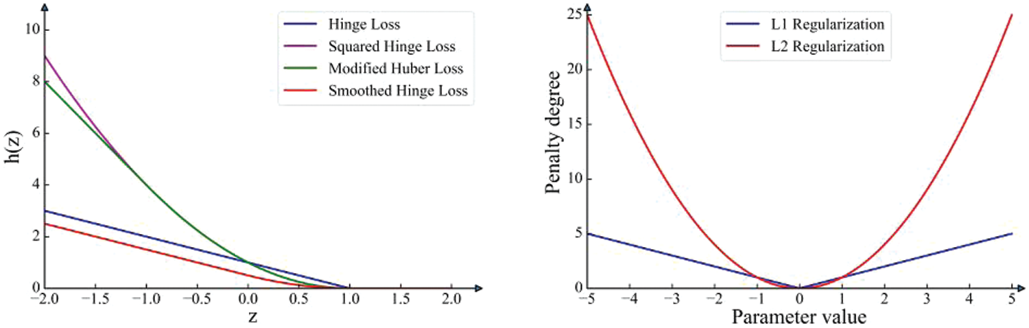
Figure 1: Loss function and regularization methods

2.3 Regularization Methods

Eq. (2), E[f(w;x)] is differentiable, even though it can be nonconvex and g(w) can exhibit both non-convexity and non-smoothness. Examples of Eq. (2) encompass sparse and low-rank learning incorporating nonconvex regularizers, e.g., Lp-norm [31], Capped-1 penalty [32] and Schatten-p norm [33]. Despite the multitude of regularization methods introduced over the years, the L1 and L2 regularization methods continue to stand out as the most widely adopted approaches. Fig. 1 illustrates these two regularization methods. It can be observed that the L2 regularization penalizes larger values more than smaller ones. This is because solutions obtained using the L2 regularization tend to be more uniform, whereas the L1 regularization often yields sparse solutions.

2.4 Proximal Gradient Descent and Its Variants

In convex optimization problems, for differentiable objective functions, we can iteratively find the optimal solution using gradient descent. However, for nondifferentiable objective functions, the introduction of sub-gradients allows us to iteratively find the optimal solution. Nevertheless, compared to gradient descent, the sub-gradient method tends to have a slower convergence rate. Therefore, for certain globally nondifferentiable but decomposable objective functions, a faster algorithm known as the proximal gradient method can be employed [34]. For a differentiable convex function F(z), assuming the starting point is x, a second-order Taylor expansion can be performed:

F(z)≈F(x)+∇F(x)T(z−x)+12∇2F(x)‖z−x‖22(8)

By substituting ∇2F(x)=1t, we obtain:

F(z)≈F(x)+∇F(x)T(z−x)+12t‖z−x‖22(9)

Minimize the quadratic approximation above:

x+=arg⁡minzF(x)+∇F(x)T(z−x)+12t‖z−x‖22(10)

The position of the next point can be obtained:

x+=x−t∇F(x)(11)

If F(z) is nondifferentiable but can be decomposed into the two functions like Eq. (2), we can still use the quadratic approximation of the smooth part f(z) to define a step towards the minimum:

x+=arg⁡minzf(z)+g(z)≈arg⁡minzf(x)+∇f(x)T(z−x)+12t‖z−x‖22+g(z)(12)

Eq. (12) can be expressed as:

x+=arg⁡minz12t‖z−(x−t∇f(x))‖22+g(x)=Proxg,t(x−t∇f(x))(13)

where Proxg,t() denotes the proximal operator with respect to the variable x and the g(x). It is also known as the iterative soft-thresholding (ISTA) function Sλt(x). When g(x)=λ‖x‖1 (the L1-norm serves as the regularization term, with the regularization parameter being λ), the soft-thresholding function is:

[Sλt(x)]i={xi−λt,if xi>λt0,if |xi|≤λtxi+λt,if xi<−λt(14)

Many scholars commonly improved the proximal gradient descent by integrating concepts such as momentum or variance reduction strategies. Li et al. [35] proposed an extension of the accelerated proximal gradient (APG) approach by introducing a monitor-corrector step to handle general nonconvex and nonsmooth programs. They are pioneering in introducing APG-type algorithms tailored for general nonconvex and nonsmooth problems. These algorithms guarantee that every accumulation point is a critical point, and they maintain convergence rates o(1/k2), particularly in convex scenarios, where k signifies the number of iterations. An accelerated proximal stochastic variance-reduced gradient (ASVRG) method with momentum acceleration was introduced by Shang et al. [36] to address objectives that are both strongly convex and non-strongly convex. Li et al. [37] introduced a proximal stochastic gradient algorithm incorporating variance reduction techniques (ProxSVRG+). This algorithm automatically transitions to faster linear convergence in certain regions, provided that the objective function locally satisfies the PL condition within those regions.

In this paper, we will consider the strategies of momentum and adaptive learning rate to further improve the performance of proximal gradient descent.

2.5 Distributed Computing on Spark

Apache Spark is extensively employed in the industrial domain, renowned for its efficacy, stability, and adept handling of intricate iterative machine-learning applications [38]. It boosts Hadoop’s performance by utilizing Resilient Distributed Datasets (RDDs), a memory-based storage system. This approach optimizes data storage between Map and Reduce iterations, resulting in enhanced efficiency and effectiveness. Due to its speed of 10~100 times faster than Hadoop, it has been rapidly adopted, especially in machine learning [39]. Within the Spark context, the driver of Spark applications functions akin to a specialized parameter server, responsible for synchronizing the update and distribution of parameters.

In Spark, data is loaded into RDDs, which have the characteristics of a data flow model: High fault tolerance and scalability. The most important point is that it has good elasticity [40]. Spark offers users a wide array of over 180 configurable parameters. Effectively selecting the optimal configuration automatically to ensure efficient execution of Spark applications poses a significant challenge. Yet Another Resource Negotiator (YARN) [41] is a technology for resource management and job scheduling, responsible for allocating system resources to various applications in Hadoop clusters and scheduling tasks to different cluster nodes. Unlike MapReduce, YARN can dynamically allocate resources for applications based on their requirements. This dynamic allocation greatly enhances resource utilization and program performance.

3  Proposed Methodology

3.1 L1 SVM with Smooth Hinge Loss

Fig. 1 presents four loss functions of SVM, clearly indicating that squared hinge loss and modified huber loss are more vulnerable to noise. Smoothed hinge loss can maintain a relatively small loss value at each iteration, making the optimization process smoother. Given the favorable properties of the smoothed hinge loss function, it will serve as the loss function for our SVM. Fig. 1 depicts two regularization images, due to the higher penalty of L2 regularization, the fluctuation amplitude during the descent process will be slightly larger. Fig. 2 illustrates the parameter changes under the proximal operator for the two types of regularization. The X-axis of the left graph represents the values of model parameters, while the Y-axis represents the magnitude of the constraints imposed by the proximal operator of the two types of regularization. On the right graph, the X-axis provides the values of 40 model parameters, and the Y-axis represents the values of these parameters after being constrained by the proximal operator of the two types of regularization. From the perspective of parameters, proximal L1 regularization tends to induce sparsity in the parameters. It prefers penalizing weights with higher absolute values compared to L2 regularization and tends to shrink other coefficients toward zero.

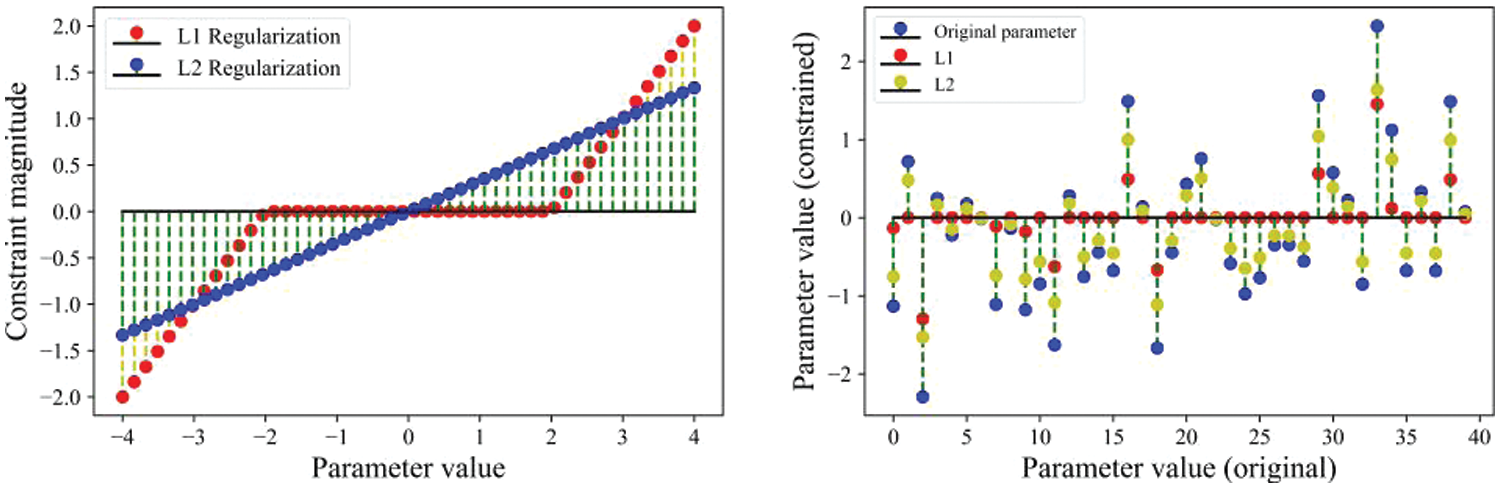
Figure 2: The effects of the two regularization methods

In the process of distributed computing, each node needs to communicate after completing its task. If the parameters are too dense, it will require more time. As analyzed in Section 2.3, L2 regularization penalizes larger values more than smaller values. This is because solutions obtained using L2 regularization tend to be more uniform, while L1 regularization typically produces sparse solutions. Therefore, in cases where the difference in accuracy is not significant, the L1 regularization method can achieve a greater advantage in distributed computing. Finally, the loss function that SVM needs to optimize is formulated as follows:

minw,b∑i=1nhs_h[1−yi(w⋅xi+b)]+λ‖w‖1(15)

where hs_h represents the smoothed hinge loss function illustrated in Eq. (7).

3.2 The Accelerated Proximal Gradient Descent with Adaptive Learning Rate and Momentum

As analyzed in Section 2.4, the proximal gradient method is faster compared to the traditional gradient descent method. By integrating concepts such as momentum or variance reduction strategies to improve the proximal gradient descent, the convergence speed can be further accelerated. Therefore, we will consider strategies such as momentum and adaptive learning rates to further enhance the performance of the proximal gradient descent. The following are specific methods.

We assume that E[f(w;x)]=f(w) in Eq. (2) has an L-Lipschitz continuous gradient for all i∈[n], there is a constant L such that:

‖∇fi(a)−∇fi(b)‖2≤L‖x−y‖2(16)

Note that fi(w)=hs_h[1−yi(w⋅xi+b)] in Eq. (15) is convex, but it is unnecessary for it to be convex. Furthermore, assuming the well-structured nature of the nonsmooth convex function in Eq. (2), we can efficiently compute its proximal operator using Eq. (13). The details of the original proximal gradient descent are described in Algorithm 1.

The Lipschitz constant L is crucial for the convergence and stability of the algorithm. In general, a smaller learning rate is chosen when the Lipschitz constant is larger to maintain stability.

Backtracking is one of the commonly used methods to determine the Lipschitz constant L. Calculating the Lipschitz constant L typically involves a global or local analysis of the objective function, which may incur significant computational costs. Particularly in high-dimensional spaces or complex functions, determining the Lipschitz constant L can be quite challenging. Therefore, in large-scale machine learning, employing adaptive learning rate methods is essential. Among the series of SGD algorithms, Adaptive moment estimation (Adam) stands out as a widely employed optimization algorithm in both machine learning and deep learning domains. It maintains an exponentially decaying average of previous gradients, akin to the momentum optimization technique. This helps smooth out the optimization path and speed up convergence. Adam adapts the learning rates of each parameter by combining the ideas of momentum and root mean square propagation (RMSprop). It dynamically adapts the learning rates by leveraging historical gradients and squared gradients, resulting in accelerated convergence and enhanced performance. The update rule for each parameter in Adam is given by:

{mk=β1mk−1+(1−β1)gkvk=β2vk−1+(1−β2)gk2m^k=mk1−β1k,v^k=vk1−β2kwk=wk−1−ηv^k+εm^k(17)

where mk, vk represent the first and second-moment estimations of the stochastic gradient.

Combining this parameter update step with Algorithm 1, Adam not only avoids the step of calculating Lipschitz constant L but also allows for algorithm acceleration through momentum. Beck et al. [42] introduced an improved iterative shrinkage-thresholding algorithm. We integrated this method with Algorithm 2. The details of the new algorithm are described in Algorithm 2 and Algorithm 3.

3.3 Synchronous Computation in Distributed Framework

From the analysis in Section 2.5, it is evident that Spark’s distributed computing is efficient, stable, and capable of handling complex algorithms proficiently. Therefore, we consider applying the adaptive proximal stochastic gradient descent L1-smoothed support vector machine to the distributed computing framework to improve detection speed and enhance detection accuracy. The following is a detailed description of the distributed method used in this paper. The mainstream communication methods are Synchronous and Asynchronous communication. They have their advantages and disadvantages. The synchronization method is susceptible to slowdowns caused by slower work nodes. Asynchronous methods introduce the issue of ‘delay’, resulting in subpar convergence performance during training. For instance, if one work node progresses quickly and has already completed 100 rounds ahead of the global model, while another node progresses slowly and is only 10 rounds ahead of the same global model, the latter’s outdated local model (or gradient) written to the parameter server is likely to impede the convergence rate of the global model. In extreme cases, Asynchronous communication may cause a very large delay, which will lead to slow convergence of the learning process. Therefore, this paper uses synchronous communication to implement the algorithm.

Fig. 3 illustrates the process of synchronously performing random gradient descent on Spark. Initially, it broadcasts either the initial weights or weights computed from previous iterations to each computing node, which can manage one or more partitions of the dataset. Following this, the input RDD is sampled based on the small batch rate. Subsequently, gradients are calculated for each sample within each partition, and the driver aggregates all gradients using a multi-pass tree reduction technique, known as TreeAggregate. The biggest feature of synchronization algorithms is that there is an explicit global synchronization state during the communication process, which is called a synchronization barrier. When a work node reaches the synchronization barrier, it enters a waiting state until all other work nodes reach the synchronization barrier. Next, different work nodes will carry out the next round of model training based on this, and in this way, one synchronization will follow the next, running repeatedly. The details of distributed PGD is shown in Algorithm 4.

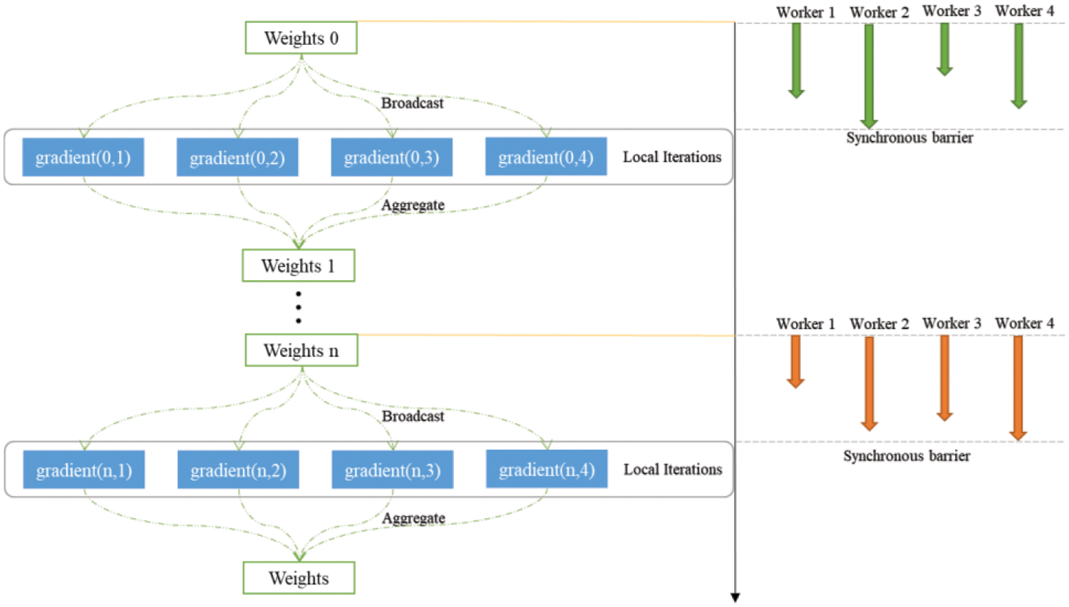
Figure 3: Synchronous computation in distributed framework

4  Experiment and Results

4.1 Experiment Setup

We conduct our experiments on a cluster comprising 1 NameNode and 3 DataNodes. Each node is equipped with a 2-core Intel (R) Core (TM) i7-10700 CPU and 16 GB of memory. Our Spark cluster runs on CentOS Linux Server 7, Java Development Kit 1.8, Apache Hadoop 3.3.0, Apache Spark 3.2.0, and Python 3.9.

4.2 Data Profile

The brain tumor MRI data utilized in this paper is publicly accessible via the figshare database, uploaded by [43]. The raw image data were acquired using T1-weighted contrast-enhanced brain images (Contrast Enhanced MRI, CE-MRI). This dataset comprises 3064 MR images from 233 patients, encompassing three types of brain tumors: 708 meningiomas, 1426 gliomas, and 930 pituitary tumors, as depicted in Fig. 4. This figure illustrates the MRI brain tumor from three different perspectives, with each image having a pixel value of 512 × 512.

Figure 4: Three types of brain tumors: Meningioma, Glioma, and Pituitary

4.3 Feature Extraction

Histogram of Oriented Gradient (HOG) is a feature descriptor employed in computer vision and image processing for object detection. It constructs features by computing and analyzing gradient direction histograms of local image regions. Firstly, we should unify the size of brain tumor images. To reduce computational complexity, we have set the size of the images to 256×256. To mitigate local shadows and minimize the influence of noise in the image, it is also necessary to standardize the uniformly sized image. The formula for normalized Gamma compression is I(x,y)=I(x,y)γ, where γ is a constant. Then calculate the pixel gradient, horizontal gradient, and vertical gradient for each grayscale image. The gradient calculation method for pixel points is as follows:

Gx(x,y)=H(x+1,y)−H(x−1,y)Gy(x,y)=H(x,y+1)−H(x,y−1)(18)

where Gx(x,y),Gy(x,y),H(x,y) respectively represent the horizontal gradient, vertical gradient, and pixel value at the pixel point (x,y).

The gradient amplitude and gradient direction at the pixel point (x,y) are as follows:

G(x,y)=Gx(x,y)2+Gy(x,y)2θG(x,y)=arctan⁡Gx(x,y)Gy(x,y)(19)

Following that, the image is partitioned into multiple cells, each with a predetermined pixel size. These cells are then treated as blocks, and the gradient histogram of each block is computed. After multiple experiments, we ultimately extracted 24,336 features from each image.

4.4 Multi-Class L1 SVM with Smooth Hinge Loss

Fig. 5 illustrates the entire experimental process. After inputting the image, features are extracted using the HOG algorithm. Subsequently, the extracted features are inputted into the classifier, and finally, our proposed algorithm is employed to solve the classifier and obtain the output result.

Figure 5: Process of the experiment

For multi-class classification problems, SVM solves them by constructing multiple binary classifiers, which can be extended by the following two strategies: One-vs.-One (O-vs.-O) strategy and One-vs.-Rest (O-vs.-R) strategy. O-vs.-O: For k categories, each time two categories are selected for training, there will be Ck2 classifiers. During testing, each classifier classifies the input, and the final class is determined through voting or another method. O-vs.-R: k binary classifiers are constructed, with each classifier distinguishing one category from all others. During testing, each classifier classifies the input, and the final class is chosen based on the highest confidence. Both methods are applicable in multi-class SVM, and the selection depends on the particular problem and requirements at hand.

In fast brain tumor detection, k = 3, the number of classifiers required for both strategies is the same. Therefore, we choose an appropriate multi-classification strategy based on the distribution of data in each category. As shown in Fig. 6, there is a relatively large number of images in the category Glioma, and if the O-vs.-R strategy is adopted, a severe imbalance issue may arise. To address this problem, it is necessary to perform class balancing before each classifier classification. To reduce computational complexity, we will adopt the O-vs.-O strategy. However, when training the classifier (Meningioma vs. Glioma), a significant class imbalance issue still arises. Therefore, we employed the synthetic minority over-sampling technique (SMOTE) balancing method when training this classifier.

Figure 6: The distribution of data

4.5 Performance Evaluation

This paper chooses Accuracy, Precision, Recall, and F1-score as the evaluation metrics for the algorithm. The calculation method is outlined as follows:

Accuracy=TP+TNTP+TN+FP+FN(20)

Prercision=TPTP+FP(21)

Recall=TPTP+FN(22)

f1−score=2∗precision∗recallprecision+recall(23)

in which TP (True Positive) represents the number of correctly predicted positive cases, indicating they are positive. TN (True Negative) represents the number of correctly predicted negative cases, indicating they are negative. FN (False Negative) is the count of negative predicted cases that are positive, referred to as Type II error. FP (False Positive) is the count of predicted positive cases that are negative, referred to as Type I errors. Precision and Recall are interdependent. Ideally, both metrics should be high; however, high precision often results in low recall, and conversely, high recall tends to lead to low precision.

4.6 Performance of Our Algorithms on a Single Node

We will use the improved algorithms (Algorithm 2 and Algorithm 3) to train each O-vs.-O SVM classifier. Fig. 7 illustrates the performance of each classifier in terms of loss and accuracy under the two algorithms. It can be observed that our Meningioma vs. Glioma classifier performs well on the training set but exhibits a lower accuracy on the test set. The remaining two classifiers show a small difference in accuracy between the training and test sets. This is likely due to the imbalance in the number of samples between Meningioma and Glioma. From the perspective of loss, the new accelerated proximal gradient descent algorithm (APGD) exhibits a faster decrease, while PGD experiences a certain slowdown in the mid-iterations. However, after the deceleration phase, PGD experiences a subsequent acceleration process. Moreover, compared to APGD, the descent of the loss becomes more significant.

Figure 7: Performance of our algorithms on a single node (PGD refers to our proposed Algorithm 2, and APGD refers to our proposed Algorithm 3)

As shown in Fig. 8, we visualize the confusion matrices of the multi-class SVM on the test set under the two algorithms. It is evident that the multi-class SVM classification performance is superior under PGD, especially in the classification of category Glioma and Pituitary, where there are only 3 errors in the classification of Pituitary. This could be attributed to APGD preserving too much momentum, allowing it to accelerate continuously but making it more prone to missing the optimal solution. It can be inferred that simply accelerating the algorithm does not necessarily lead to optimal model performance. While considering the loss, we also need to balance the performance of the model. Therefore, in the next experiments, we will implement distributed synchronous computation based on PGD (Algorithm 2).

Figure 8: Confusion matrix of our algorithms (PGD refers to our proposed Algorithm 2, and APGD refers to our proposed Algorithm 3, distributed PGD refers to our proposed Algorithm 4)

4.7 Performance of Distributed PGD

The details of the distributed synchronous computation PGD have been presented. Next, we will use this algorithm to train each O-vs.-O SVM classifier. Fig. 9 illustrates the performance of each classifier in terms of loss and accuracy. It can be observed that the performance of the Meningioma vs. Glioma classifier under the DPGD algorithm is closer between the testing and training sets (compared to Fig. 7). From the perspective of loss, DPGD can achieve lower loss in a shorter number of iterations. For instance, in the optimization of the Meningioma vs. Glioma classifier, it can stabilize the loss around 0.68 by the 30th iteration, whereas PGD requires more than 100 iterations to achieve the same result. Additionally, comparing Figs. 7 and 9, the loss curve under DPGD is smoother, making it less prone to oscillations in the later iterations.

Figure 9: Performance of distributed PGD

As shown in Fig. 8, we visualize the confusion matrices of the multi-class SVM on the test set under the DPGD algorithm. The classification performance of the L1 SVM under DPGD and PGD algorithms is very close. The model under the PGD excels in recognizing Meningioma brain tumors, while the model under DPGD demonstrates more precise recognition of Pituitary brain tumors. The recognition accuracy for Glioma brain tumors is the same under both algorithms.

The performance of the L1 SVM models under these algorithms we proposed in other aspects (i.e., Precision, Recall, F1-score) is shown in Table 1. The performance of L1 SVM with PGD and L1 SVM with DPGD is also quite similar in other aspects. In Table 2, we compare the running times of PDG and DPGD for various classifiers over 200 iterations. It can be observed that, at the same number of iterations, the distributed framework algorithm has a slightly shorter running time. However, the difference between the two is not significant; for example, in the case of Meningioma vs. Glioma, the difference between the two algorithms is only 2.31 s. However, the algorithm under the distributed framework converges faster, requiring fewer iterations to achieve the same result.

4.8 Comparison of Our Work and Related Works

The performance of the aforementioned proposed models is outlined in Table 1. The performance of the L1 support vector machine with PGD and the L1 support vector machine with DPGD is very similar in all aspects of the table. In Table 2, we compare the running time of PDG and DPGD for various classifiers over 200 iterations. It can be observed that the running time of the distributed framework algorithm is slightly shorter at the same number of iterations. However, the difference between the two is not significant; for example, the difference between the two algorithms in the case of meningioma and glioma is only 2.31 s. Nevertheless, the algorithm under the distributed framework converges faster and requires fewer iterations to achieve the same result. In Table 3, we contrast the accuracy of the proposed model in this paper with that of models found in related literature. It can be seen that the momentum distribution adaptive proximal stochastic gradient descent L1-smoothed support vector machine model proposed in this paper performs excellently, achieving an accuracy of 95.21%.

After compiling and summarizing the related work and conducting a comparative analysis with our own work, the results are presented in Table 3. Several researchers and practitioners have introduced various algorithms for brain tumor detection. Our study offers the following enhancements:

(i) Compared to traditional SVM, our L1 SVM demonstrates superior classification performance. The smoothed hinge loss preserves the characteristics of the original hinge function, and its gradient is more readily computable. Additionally, the proximal gradient algorithm proposed by us can exhibit faster speed compared to the subgradient method.

(ii) Deep learning methods have complex network structures. The more layers a network has, the greater the number of parameters the algorithm needs to optimize, leading to longer computation times. Compared to them, SVM requires a significantly smaller number of parameters to optimize. Building upon this, we further propose an L1 SVM that allows for sparse parameters. In a distributed computing framework, our algorithm exhibits even more pronounced advantages.

5  Conclusion and Future Work

Our research on fast brain tumor detection not only validates the effectiveness of Algorithm 2 and Algorithm 4 but also demonstrates that our detection method achieves higher accuracy in less time compared to other algorithms. We observe that in the distributed computing framework, communication incurs a significant time cost. Communication cost is primarily determined by the number of parameters, and traditional machine learning models have fewer parameters compared to deep learning models. The L1-smoothed SVM we proposed can achieve comparable accuracy in practical applications to deep learning models with a large number of parameters. To address the nonsmooth nature of L1 regularization, we propose an adaptive PGD algorithm with momentum. Applying the improved algorithm to a distributed framework, the results indicate that the proposed method not only ensures the desired accuracy but also accelerates computation and reduces time costs. This means that when dealing with large-scale medical imaging datasets, the algorithm can utilize computational resources more efficiently, thereby improving data processing throughput.

In future endeavors, we aim to enhance fast brain tumor detection through two separate approaches. Firstly, stochastic algorithms utilize the gradient of a single sample or a small batch of samples as an unbiased estimate for the entire dataset. This introduces significant variance. In the subsequent stages, we will consider incorporating variance reduction strategies to further enhance our algorithm. Secondly, there are various ways to reduce communication costs, and we will consider employing a distributed topology structure to further decrease communication overhead.

Acknowledgement: None.

Funding Statement: This work was supported in part by the Natural Science Foundation of Ningxia Province (No. 2021AAC03230). The authors would like to thank the anonymous reviewers for their valuable comments and suggestions.

Author Contributions: The authors confirm contribution to the paper as follows: study conception and design: Chuandong Qin, Yu Cao; data collection: Chuandong Qin, Yu Cao; analysis and interpretation of results: Chuandong Qin, Yu Cao; draft manuscript preparation: Chuandong Qin, Yu Cao, Liqun Meng. All authors reviewed the results and approved the final version of the manuscript.

Availability of Data and Materials: This study used the publically available dataset: https://figshare.com/articles/dataset/brain_tumor_dataset/1512427.

Conflicts of Interest: The authors declare that they have no conflicts of interest to report regarding the present study.

References

1. S. Y. Zhao, Y. P. Xie, and W. J. Li, “On the convergence and improvement of stochastic normalized gradient descent,” Sci. China Inf. Sci., vol. 64, no. 3, pp. 1–13, 2021. doi: 10.1007/s11432-020-3023-7. [Google Scholar] [CrossRef]

2. M. A. Zinkevich, M. Weimer, A. Smola, and L. Li, “Parallelized stochastic gradient descent,” Adv. Neur. Inf. Process. Syst, vol. 21, pp. 1–9, 2010. [Google Scholar]

3. E. P. Xing et al., “Petuum: A new platform for distributed machine learning on big data,” IEEE Trans. Big Data, vol. 2, no. 1, pp. 49–67, 2015. [Google Scholar]

4. S. Sra, A. W. Yu, M. Li, and A. J. Smola, “AdaDelay: Delay adaptive distributed stochastic optimization,” in Int. Conf. Artif. Intell. Stat., 2016, pp. 957–965. [Google Scholar]

5. D. Cheng, S. Li, and Y. Zhang, “WP-SGD: Weighted parallel SGD for distributed unbalanced-workload training system,” J. Parallel. Distr. Comput., vol. 145, no. 1, pp. 202–216, 2020. doi: 10.1016/j.jpdc.2020.06.011. [Google Scholar] [CrossRef]

6. F. Shang, H. Huang, J. Fan, Y. Liu, H. Liu and J. Liu, “Asynchronous parallel, sparse approximated SVRG for high-dimensional machine learning,” IEEE Trans. Knowl. Data Eng., vol. 34, no. 12, pp. 5636–5648, 2021. doi: 10.1109/TKDE.2021.3070539. [Google Scholar] [CrossRef]

7. P. J. Huber, “Robust estimation of a location parameter,” Breakthr. Statist.: Methodol. Distribut., vol. 35, pp. 492–518, 1992. doi: 10.1007/978-1-4612-4380-9_35. [Google Scholar] [CrossRef]

8. T. Zhang and F. J. Oles, “Text categorization based on regularized linear classification methods,” Inf. Retr., vol. 4, no. 1, pp. 5–31, 2001. doi: 10.1023/A:1011441423217. [Google Scholar] [CrossRef]

9. J. D. Rennie and N. Srebro, “Loss functions for preference levels: Regression with discrete ordered labels,” in Proc. IJCAI Multidiscipl. Workshop Adv. Prefer. Handl., Menlo Park, CA, USA, AAAI Press, vol. 1, 2005. [Google Scholar]

10. P. Gong, C. Zhang, Z. Lu, J. Huang, and J. Ye, “A general iterative shrinkage and thresholding algorithm for non-convex regularized optimization problems,” in Int. Conf. Mach. Learn., 2013, pp. 957–965. [Google Scholar]

11. R. I. Boţ, E. R. Csetnek, and S. C.László, “An inertial forward-backward algorithm for the minimization of the sum of two nonconvex functions,” EURO J. Comput. Opt., vol. 4, no. 1, pp. 3–25, 2016. doi: 10.1007/s13675-015-0045-8. [Google Scholar] [CrossRef]

12. Q. Li, Y. Zhou, Y. Liang, and P. K. Varshney, “Convergence analysis of proximal gradient with momentum for nonconvex optimization,” in Int. Conf. Mach. Learn., 2017, pp. 2111–2119. [Google Scholar]

13. N. Zulpe and V. Pawar, “GLCM textural features for brain tumor classification,” Int. J. Comput. Sci. Issues (IJCSI), vol. 9, no. 3, pp. 354, 2012. [Google Scholar]

14. J. Jiang, Y. Wu, M. Huang, W. Yang, W. Chen and Q. Feng, “3D brain tumor segmentation in multimodal MR images based on learning population- and patient-specific feature sets,” Comput. Med. Imag. Grap., vol. 37, no. 7–8, pp. 512–521, 2013. doi: 10.1016/j.compmedimag.2013.05.007. [Google Scholar] [PubMed] [CrossRef]

15. A. Kumar, P. Chauda, and A. Devrari, “Machine learning approach for brain tumor detection and segmentation,” Int. J. Org. Collect. Intell. (IJOCI), vol. 11, no. 3, pp. 68–84, 2021. doi: 10.4018/IJOCI.2021070105. [Google Scholar] [CrossRef]

16. R. Ranjbarzadeh, A. Caputo, E. B. Tirkolaee, S. J. Ghoushchi, and M. Bendechache, “Brain tumor segmentation of MRI images: A comprehensive review on the application of artificial intelligence tools,” Comput. Biol. Med., vol. 152, no. 4, pp. 106405, 2023. doi: 10.1016/j.compbiomed.2022.106405. [Google Scholar] [PubMed] [CrossRef]

17. A. Bagherian Kasgari, R. Ranjbarzadeh, A. Caputo, S. Baseri Saadi, and M. Bendechache, “Brain tumor segmentation based on zernike moments, enhanced ant lion optimization, and convolutional neural network in MRI Images,” Metaheur. Opt. Comput. Electr. Eng., vol. 2, pp. 345–366, 2023. [Google Scholar]

18. M. Uvaneshwari and M. Baskar, “Computer-aided diagnosis model using machine learning for brain tumor detection and classification,” Comput. Syst. Sci. Eng., vol. 46, no. 2, pp. 1811–1826, 2023. doi: 10.32604/csse.2023.035455. [Google Scholar] [CrossRef]

19. U. Javed, M. M. Riaz, A. Ghafoor, and T. A. Cheema, “MRI brain classification using texture features, fuzzy weighting and support vector machine,” Progress Electromag. Res. B, vol. 53, pp. 73–88, 2013. [Google Scholar]

20. N. N. Gopal and M. Karnan, “Diagnose brain tumor through MRI using image processing clustering algorithms such as Fuzzy C Means along with intelligent optimization techniques,” in 2010 IEEE Int. Conf. Comput. Intell. Comput. Res., IEEE, 2010, pp. 1–4. [Google Scholar]

21. J. Amin, M. Sharif, M. Yasmin, and S. L. Fernandes, “A distinctive approach in brain tumor detection and classification using MRI,” Pattern Recogn. Lett., vol. 139, no. 14, pp. 118–127, 2020. doi: 10.1016/j.patrec.2017.10.036. [Google Scholar] [CrossRef]

22. A. K. Anaraki, M. Ayati, and F. Kazemi, “Magnetic resonance imaging-based brain tumor grades classification and grading via convolutional neural networks and genetic algorithms,” Biocybern. Biomed. Eng., vol. 39, no. 1, pp. 63–74, 2019. doi: 10.1016/j.bbe.2018.10.004. [Google Scholar] [CrossRef]

23. M. Khan, S. A. Shah, T. Ali, A. Khan Quratulain, and G. S. Choi, “Brain tumor detection and segmentation using RCNN,” Comp., Mater. Contin., vol. 71, no. 3, pp. 5005–5020, 2022. doi: 10.32604/cmc.2022.023007. [Google Scholar] [CrossRef]

24. Z. N. K. Swati et al., “Brain tumor classification for MR images using transfer learning and fine-tuning,” Comput. Med. Imag. Grap., vol. 75, pp. 4–46, 2019. doi: 10.1016/j.compmedimag.2019.05.001. [Google Scholar] [PubMed] [CrossRef]

25. R. Ranjbarzadeh, A. B. Kasgari, S. J. Ghoushchi, S. Anari, M. Naseri and M. Bendechache, “Brain tumor segmentation based on deep learning and an attention mechanism using MRI multi-modalities brain images,” Sci. Rep., vol. 11, no. 1, pp. 10930, 2021. doi: 10.1038/s41598-021-90428-8. [Google Scholar] [PubMed] [CrossRef]

26. M. Ali et al., “Brain tumor detection and classification using pso and convolutional neural network,” Comput., Mater. Contin., vol. 73, no. 3, pp. 4501–4518, 2022. doi: 10.32604/cmc.2022.030392. [Google Scholar] [CrossRef]

27. C. Qin, B. Li, and B. Han, “Fast brain tumor detection using adaptive stochastic gradient descent on shared-memory parallel environment,” Eng. App. Artif. Intell, vol. 120, pp. 105816, 2023. [Google Scholar]

28. R. Gurusamy and V. Subramaniam, “A machine learning approach for MRI brain tumor classification,” Comput., Mater. Contin., vol. 53, no. 2, pp. 91–108, 2017. [Google Scholar]

29. H. S. Suresha and S. S. Parthasarathy, “Alzheimer disease detection based on deep neural network with rectified adam optimization technique using MRI analysis,” in 2020 Third Int. Conf. Adv. Electr., Comput. Commun. (ICAECC), 2020. [Google Scholar]

30. A. Kumar, “Study and analysis of different segmentation methods for brain tumor MRI application,” "Multimed. Tools App., vol. 82, no. 5, pp. 7117–7139, 2023. [Google Scholar]

31. S. Foucart and M. J. Lai, “Sparsest solutions of underdetermined linear systems via ℓq-minimization for0 < q ⩽ 1,” Appl. Comput. Harmon. Anal., vol. 26, no. 3, pp. 395–407, 2009. [Google Scholar]

32. T. Zhang, “Analysis of multi-stage convex relaxation for sparse regularization,” J. Mach. Learn. Res., vol. 11, no. 3, pp. 1–27, 2010. [Google Scholar]

33. K. Mohan and M. Fazel, “Iterative reweighted algorithms for matrix rank minimization,” J. Mach. Learn. Res., vol. 13, no. 1, pp. 3441–3473, 2012. [Google Scholar]

34. Z. Lin, H. Li, and C. Fang, “Accelerated algorithms for nonconvex optimization,” in Accelerated Optimization for Machine Learning. Nature Singapore: Springer, 2020, pp. 109–137. [Google Scholar]

35. H. Li and Z. Lin, “Accelerated proximal gradient methods for nonconvex programming,” Adv. Neur. Inf. Process. Syst., vol. 28, pp. 1–9, 2015. [Google Scholar]

36. F. Shang, L. Jiao, K. Zhou, J. Cheng, Y. Ren and Y. Jin, “ASVRG: Accelerated proximal SVRG,” in Asian Conf. Mach. Learn., 2018, pp. 815–830. [Google Scholar]

37. Z. Li and J. Li, “A simple proximal stochastic gradient method for nonsmooth nonconvex optimizatio,” Adv. Neur. Inf. Process. Syst., vol. 31, pp. 1–11, 2018. [Google Scholar]

38. M. Zaharia, M. Chowdhury, M. J. Franklin, S. Shenker, and I. Stoica, “Spark: Cluster computing with working sets,” in 2nd USENIX Workshop Hot Topics Cloud Comput (HotCloud 10), 2010. [Google Scholar]

39. D. Cheng, X. Zhou, P. Lama, J. Wu, and C. Jiang, “Cross-platform resource scheduling for spark and mapreduce on yarn,” IEEE Trans. Comput., vol. 66, no. 8, pp. 1341–1353, 2017. [Google Scholar]

40. H. Zhang, Z. Liu, H. Huang, and L. Wang, “FTSGD: An adaptive stochastic gradient descent algorithm for spark mllib,” in 2018 IEEE 16th Intl. Conf. Depend., Autono. Secur. Comput., 16th Intl. Conf. Perv. Intell. Comput., 4th Intl. Conf. Big Data Intell. Comput. Cyber Sci. Tech. Congress (DASC/PiCom/DataCom/CyberSciTech), IEEE, 2018. [Google Scholar]

41. Z. Yang et al., “AutoAdmin: Automatic and dynamic resource reservation admission control in Hadoop YARN clusters,” Scal. Comput.: Pract. Exp., vol. 19, no. 1, pp. 53–68, 2018. doi: 10.12694/scpe.v19i1.1393. [Google Scholar] [CrossRef]

42. A. Beck and M. Teboulle, “A fast iterative shrinkage-thresholding algorithm for linear inverse problems,” SIAM J. Imag. Sci., vol. 2, no. 1, pp. 183–202, 2009. doi: 10.1137/080716542. [Google Scholar] [CrossRef]

43. J. Cheng et al., “Enhanced performance of brain tumor classification via tumor region augmentation and partition,” PLoS One, vol. 10, no. 10, pp. e0140381, 2015. doi: 10.1371/journal.pone.0140381. [Google Scholar] [PubMed] [CrossRef]

44. M. R. Ismael and I. Abdel-Qader, “Brain tumor classification via statistical features and back-propagation neural network,” in 2018 IEEE Int. Conf. Electro/Inf. Tech. (EIT), IEEE, 2018, pp. 0252–0257. [Google Scholar]

45. P. Afshar, K. N. Plataniotis, and A. Mohammadi, “Capsule networks for brain tumor classification based on MRI images and coarse tumor boundaries,” in ICASSP 2019–2019 IEEE Int. Conf. Acoust., Speech Signal Process. (ICASSP), IEEE, 2019, pp. 1368–1372. [Google Scholar]