Improved Particle Swarm Optimization for Parameter Identification of Permanent Magnet Synchronous Motor

Nomenclature

1  Introduction

Because the stator resistance, d/q axis inductance, flux linkage, and other motor parameters are readily influenced by temperature, stator current, magnetic saturation, and other factors, the control performance of high-performance PMSM, reliability, and system dynamic and static performance are all negatively impacted. Therefore, precisely identifying the PMSM parameters is required to achieve high-performance PMSM control or reliable fault diagnosis [1–5].

Numerous scholars have undertaken comprehensive investigations into diverse techniques for ascertaining PMSM parameters. These techniques can be classified into two groups, namely offline identification and online identification, according to distinct identification procedures [6]. The two primary offline identification techniques for PMSM parameters are experimental measurement and finite element analysis. One approach that is frequently used to determine the PMSM parameters is finite element analysis [6].

The online identification approach is superior than the offline identification method because it allows for real-time modification of controller parameters for adaptive control in addition to real-time monitoring of the motor’s operational state. As a result, researchers have undertaken a great deal of research in this area, producing successful findings and a variety of online identification techniques, including the Kalman filter algorithm [7,8], the recursive least square method [9–11], model reference adaptive algorithm [12,13], and artificial intelligence algorithm. These methods enable single-parameter or multi-parameter online identification of PMSM.

Although the recursive least squares algorithm is more susceptible to measurement noise, it has a reasonable computational complexity. The model reference adaptive algorithm can guarantee the asymptotic convergence of the detected parameters based on stability analysis. However, it is challenging to find an adaptive law that satisfies stability requirements when identifying numerous factors at once; this process involves a great deal of trial and error, and measurement noise can readily impact the identification results. In noisy situations, Extended Kalman filters (EKF) can offer state estimation in the sense of lowest variance. The parameters that need to be recognized must, nevertheless, be treated as state variables, which in some systems can be complicated.

In [14–16], PSO was adopted to achieve full-parameter identification of electrical parameters. In reference [17], an immune clone differential algorithm was proposed to identify four electrical parameters of PMSM. The identification accuracy and dynamic convergence speed of the algorithm are taken into account, and the algorithm has better global searching ability. An adaline neural network algorithm was proposed in reference [18] to identify multiple parameters simultaneously. However, the algorithm’s calculation process was relatively complex, and it failed to account for the impact of inductance changes brought about by injection current-induced changes in the motor’s magnetic circuit on identification accuracy.

The method of parameter identification for PMSM outlined in reference [19] is based on chaotic particle swarm optimization with dynamic self-optimization (DSCPSO), which estimates the parameters and nonlinearity of the voltage source inverter (VSI) simultaneously in order to achieve real-time compensation of the VSI nonlinearity. The algorithm’s capacity to investigate perhaps better regions is improved by incorporating tent chaos theory into the updating of the population, inertia weights, and learning variables of PSO. Additionally, the resilience of the simulated annealing algorithm (SA) is paired with the enhancement of population diversity, and the memory tempering annealing (MTA) strategy is employed to assure multiple learning of particles. Dynamic lens imaging opposition-based learning (DLIOBL) and domain optimization algorithms based on evolutionary information are meant to ensure a healthy balance between development and exploration. Reference [20] proposed a new multi-strategy self-optimizing simulated annealing particle swarm optimization technique called SOSAPSO. To prevent particle swarm monotonicity, this technique introduces dynamic opposition-based learning (DOBL) during the inertia weight update phase, simplifying the velocity term of PSO. Furthermore, to achieve self-learning in deep regions, a hybrid variation technique based on density and similarity between Cauchy and Gaussian processes is devised. Simulated annealing (SA) with memory and tempering mechanism is incorporated into SOSAPSO at the same time, and when the evolution of SOSAPSO reaches a standstill, the greedy optimization algorithm (GOA) is employed to improve the local fine exploitation capability. This approach has strong resilience and convergence speed, and it can successfully avoid the local convergence problem. However, due to the excessive improvement of PSO, the algorithm is too complicated, which greatly increases the computational difficulty. A directdrive permanent magnet synchronous generator (D-PMSG) parameter determination approach based on mean particle swarm optimization with extreme disturbance (EDMPSO)-EKF is proposed in reference [21]. Initially, a dual-thread identification model is constructed by analyzing the EKF principle. Subsequently, the particle swarm optimization (PSO) algorithm is refined to exit the local optimum by incorporating extremum interference and calculating the average extremum. Ultimately, the system executes parameter identification after getting the ideal noise matrix, and the enhanced PSO method is applied to the adaptive optimization of the EKF system noise matrix and measurement noise matrix. The calculation of this method is complicated and the calculation amount is large. A multi-parameter identification technique for permanent magnet synchronous motors based on simulated annealing particle swarm optimization (MRAS-SAPSO) and a model reference adaptive system was presented in reference [22]. First, the electrical parameters of a permanent magnet synchronous motor are determined using the model reference adaptive system approach. Second, the identification motor control system’s electrical and mechanical parameters are further adjusted using the identification results as the initial population of PSO identification. The optimization results of the adaptive simulated annealing approach for multi-parameter identification are introduced in order to prevent premature convergence of PSO. This method simply uses the two algorithms successively, which not only does not avoid the shortcomings of the two algorithms, but also increases the complexity of the algorithm. A couple of enhanced PSOs have been suggested in the reference [23]. One is the combination of quasi-opposition-based learning (QOBL) with PSO, which helps to broaden and quicken the search actions. Second, the PSO’s capacity for global search is further improved by the addition of a chaotic local search. The PSO is overly complex as a result of the algorithm’s two improvements. PSO’s research focus in PMSM parameter identification is on how to fully utilize its optimization potential without burdening the algorithm with more calculations. Since intelligent algorithms are very good at nonlinear optimization, they are employed extensively. However, such algorithms have the problems of huge computational load and excessive data processing burden. Further research is needed to reduce the computational load of intelligent algorithms while ensuring identification accuracy.

Three features of the technique presented in this research help to better detect the parameters of PMSM. Initially, the PSO algorithm is combined to create a new fuzzy controller, whose fuzzy rules help to enhance the algorithm’s local and global search capabilities as well as the PSO’s premature convergence defect. This allows each particle to have a distinct rule distribution. Secondly, a transformation function is suggested to streamline the fitness function while maintaining the control object’s global optimal solution. This minimizes the likelihood of a local minimum during the optimization procedure. Thirdly, early in the optimization process, the algorithm may be able to break out of the local minimum point thanks to the freshly filled function.

2  Mathematical Model of PMSM

The PMSM possesses an ideal symmetrical structure. Neglecting the effects of magnetic field saturation, iron loss, and eddy current loss in PMSM, the axis equation of the rotating coordinate system d/q can be described as follows:

{ud=Rid+Lddiddt−ωeLqiquq=Riq+Lqdiqdt+ωe(Ldid+ψf)(1)

in the equation, ud, uq, iq, id are respectively the d/q axis voltage and current, R, ωe, ψf are respectively the stator resistance, electrical angular speed, and flux linkage.

In a VSI-fed PMSM system, The voltage equation of PMSM considering VSI nonlinearity is provided in reference [14].

{ud∗=Rid+Lddiddt−ωeLqiq−Dd(k)Vdeaduq∗=Riq+Lqdiqdt+ωe(Ldid+ψf)−Dq(k)Vdead(2)

where Dd and Dq are the functions of the rotor position period:

[Dd(k)Dq(k)]=2[cos⁡(θ)cos⁡(θ−2π3)cos⁡(θ+2π3)−sin⁡(θ)−sin⁡(θ−2π3)−sin⁡(θ−π3)]×[sign(ias)sign(ibs)sign(ics)](3)

where ias, ibs, ics are the stator abc three-phase currents, respectively.

sign={1,i≥0−1,i<0(4)

Vdead can be represented as:

Vdead=Tdead+Ton−ToffTs(Vdc−Vsat+Vd)+Vsat+Vd2(5)

where Tdead is the dead-time period, Ton, Toff are turn-on, turn-off times of the switching device.

Vdc, Vsat and Vd are respectively the DC bus voltage, the saturation voltage drop of the active switch, and the forward voltage drop of the free wheel diode. When the motor is in steady state operation, Eq. (2) can be expressed as:

{ud∗=Rid−ωeLqiq−Dd(k)Vdeaduq∗=Riq+ωe(Ldid+ψf)−Dq(k)Vdead(6)

There are five electrical parameters that need to be identified: R, Ld, Lq, ψf, Vdead. However, the order of Eq. (6) is two, so the motor equation of state is a non-full rank equation. The variables such as stator resistance, rotor flux and winding inductance change with load and temperature during motor operation, which easily lead to inaccurate identification results.

According to the principle introduced in reference [2], PMSM generally adopts id=0 strategy for decoupling flux and torque control. Under steady state conditions, by injecting a current of id≠0 into the d-axis for a short time, Eq. (6) can be transformed into a system of equations of full rank [14]:

{ud0∗(k)=−ωe(k)Lqiq0(k)−Dd0(k)Vdeaduq0∗(k)=Riq0(k)+ωe(k)ψf−Dq0(k)Vdeadud1∗(k)=Rid1(k)−ωe(k)Lqiq1(k)−Dd1(k)Vdeaduq1∗(k)=Riq1(k)+ωe(k)(Ldid1(k)+ψf)−Dq1(k)VdeadΔuq∗(k)=uq1∗(k)−uq0∗(k)=ωe(k)Ldid1(k)−Dq1(k)Vdead+Dq0(k)Vdead(7)

in the equation, the lower corner of variables and parameters collected in mode id=0 is marked with “0”, and the lower corner of variables and parameters collected in mode id≠0 is marked with “1”.

The PMSM parameter identification structure is shown in Fig. 1.

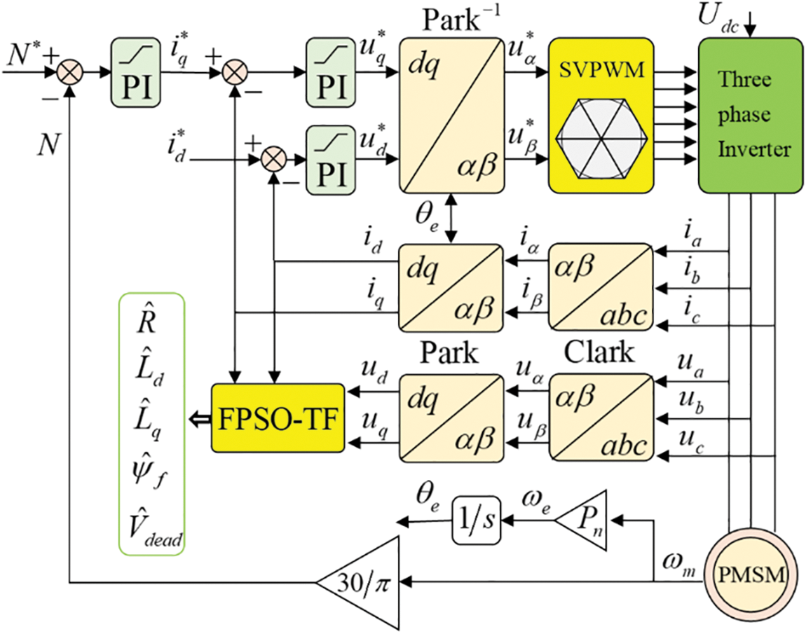
Figure 1: PMSM on-line parameter identification schematic diagram

3  Fitness Function

The identified value in the theoretical model must be continuously optimized and modified to bring it closer to the actual value until the fitness function value is the lowest. This process yields five parameters that need to be identified. The principle of parameter identification requires the output difference between the established theoretical model and the practical model that is currently in use, the calculation of the matching fitness function, and the calculation result as input to the intelligent algorithm. The schematic diagram for PMSM parameter identification based on FPSOTF is displayed in Fig. 2.

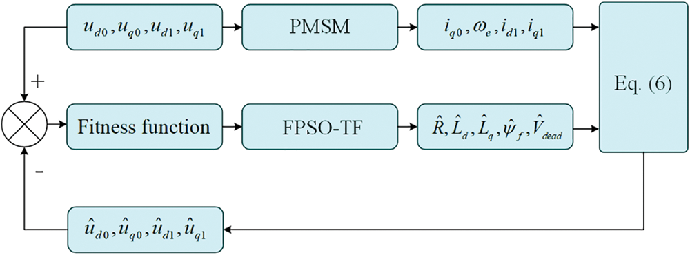
Figure 2: Principle of FPSOTF

The fitness function in this paper consists of five parts, which are defined as follows:

f1(L^q,V^dead)=1n∑k=1n(ud0∗(k)+Dd0(k)V^dead−u^d0(k))2(8)

f2(R^,ψ^f,V^dead)=1n∑k=1n(uq0∗(k)+Dq0(k)V^dead−u^q0(k))2(9)

f3(R^,L^q,V^dead)=1n∑k=1n(ud1∗(k)+Dd1(k)V^dead−u^d1(k))2(10)

f4(R^,ψ^f,L^q,V^dead)=1n∑k=1n(uq1∗(k)+Dq1(k)V^dead−u^q1(k))2(11)

f5(L^d,V^dead)=1n∑k=1n(Δuq∗(k)−L^dωe(k)id1(k)+V^dead(Dq1(k)−Dq0(k)))2(12)

the fitness function is:

f=a1f1+a2f2+a3f3+a4f4+a5f5(13)

where a1, a2, a3, a4, a5 are the weighting coefficients.

4  Algorithm Design

4.1 Multi Loop Fuzzy Control System

The optimization problem considered in this paper is:

minf(x),x∈Ω⊂Rn(14)

where f(x) is a differentiable continuous function.

4.1.1 Single Loop Control System

The single-loop control system of problem (13) is shown in Fig. 3, where f(x) is the controlled object and R is the constant input. Here T(a,b,x) is used to change the expression form of fitness function without changing the position of the extreme point of fitness function, so that the optimal value of fitness function can be separated from the local minimum, reducing the possibility of the calculation process falling into the local optimal, and making the optimization problem fast and simple. The introduction of the transformation function must ensure that the position of the extreme point before and after the fitness function transformation remains unchanged.

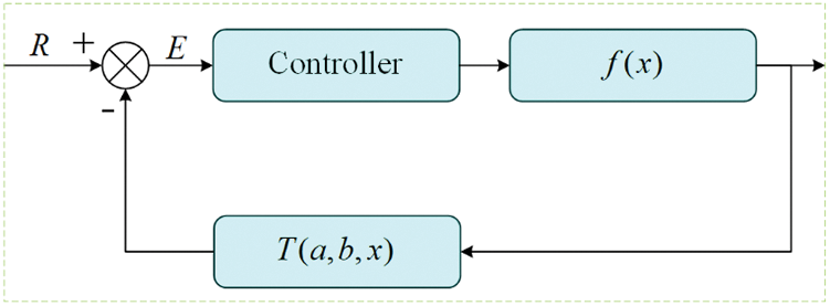
Figure 3: The single loop control system

The transformation function is:

T(a,b,x)=a(x−b)/1+(a(x−b))2,a>0(15)

Eq. (15) is a differentiable continuous function. The extreme point of the fitness function is the solution of ∂f(x)/∂x=0, the transformed function is:

T(f(x))=a(f(x)−b)/1+(a(f(x)−b))2,a>0(16)

The extreme point of Eq. (16) is the solution of Eq. (17).

∂T(f(x))/∂x=(∂T/∂f)×(∂f(x)/∂x)=0(17)

Eq. (17) can be further expressed as:

∂T/∂f=∂[a(f−b)/1+(a(f−b))2]/∂f=a/[[1+(a(f−b)2]1+(a(f−b))2]>0(18)

It can be seen from Eq. (18), ∂T/∂f>0, ∂T[f(x)]/∂x=(∂T/∂x)×(∂f(x)/∂x)=0, ∂f(x)/∂x=0, that is, T[f(x)] and f(x) have the same extreme point, and the transformation function does not change the extreme point position of the original fitness function.

As shown in Fig. 4a, when b=0, the transformation function T(a,b,x) is basically close to the proportional function near the zero point, and the value of the regional transformation function far from the zero point tends to 1. When the transformation function acts on the fitness function, the shape of the fitness function curve before and after the action changes little near zero, while the fitness function curve with the fitness function value far from zero tends to 1, and its shape changes greatly and is horizontal. The new fitness function obtained by the transformation has a global minimum point near zero, and the transformed function can reduce the possibility of falling into the local minimum point in the algorithm calculation process. The larger a is, the smaller the effective search range is. Conversely, the smaller a is, the larger the effective search range is.

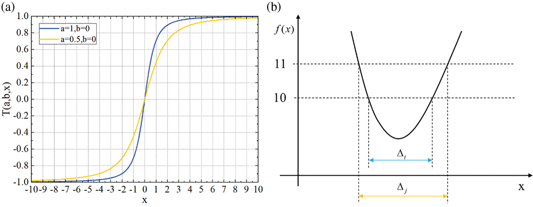
Figure 4: (a) Transformation function curve; (b) The relationship between f(x) and li

As shown in Fig. 4a, when a=1, if the independent variable of the transformation function is greater than 10, the value of the transformation function tends to 1, so the effective change interval of the independent variable is [−10,10]. As shown in Fig. 4b, when b=0, T[f(x)]=f(x)/1+f(x)2, li of function f(x)=10 has two points of intersection with function f(x), in this case, the effective search area should be Δi, when b=1, T[f(x)]=f(x)/1+(f(x)−1)2, f(x)−1=10, li of function f(x)=11 has two points of intersection with function f(x), in this case, the effective search area should be Δj, as shown in Fig. 4b, Δi<Δj, when a is held constant, the greater the value of b, the larger the effective search area Δj becomes; otherwise, when b decreases, so does the effective search area Δi.

When a=1,b=0, T(a,b,x)=T(1,0,x)=x/1+x2.

The comparison diagram after T transformation is shown in Fig. 5, in which Figs. 5a–5c are three functions (19)–(21). These three functions have multiple local extremum points, and the algorithm is easy to fall into local extremum points in the calculation process. Figs. 6a–6c are the corresponding T(f(x)) images after T transformation. It can be seen from the function image after transformation that many local extreme values in the original function are reduced, while the optimal value after transformation is better highlighted.

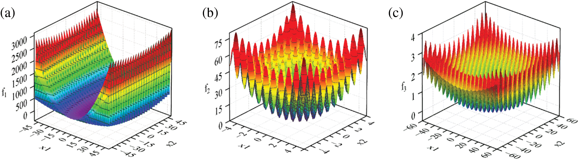
Figure 5: (a) Function of f1; (b) Function of f2; (c) Function of f3

f1=π2(10sin2⁡(π(1.25+0.25x1))+(0.25+0.25x2)2+(0.25+0.25x1)(1+10sin2⁡(π(1.25+0.25x2))))(19)

f2=x12+x22−10cos⁡(2πx1)−10cos⁡(2πx2)+20(20)

f3=14000(x12+x22)−cos⁡(x1)cos⁡(x22)+1(21)

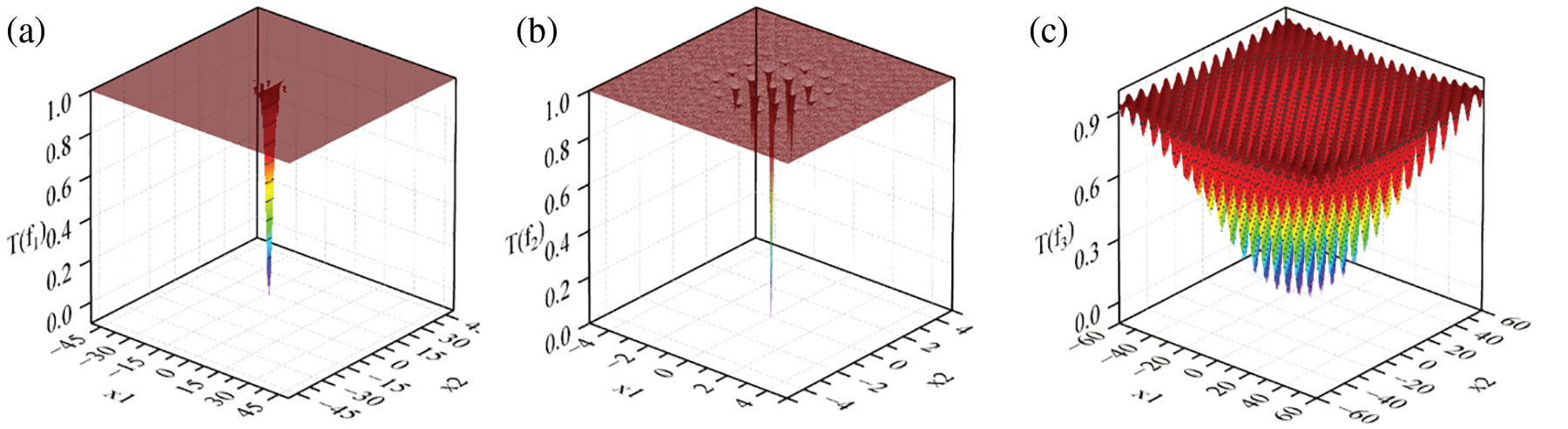
Figure 6: (a) Function of T(f1); (b) Function of T(f2); (c) Function of T(f3)

4.1.2 Multi Loop Fuzzy Control System

The multi loop fuzzy control system is shown in Fig. 7. A subsystem is equivalent to a particle, FNN1, …, FNNm is the fuzzy controller distinguished from m different membership functions, and at the same time reflects the global search ability and local search ability of the system, f(x) is the fitness function. Best(f(x)) is the optimal value of the subsystem, each subsystem shares the optimal value of all subsystems, and quickly adjusts the optimization direction of the subsystem according to the shared information. min(f(x)) is the optimal value of the entire system.

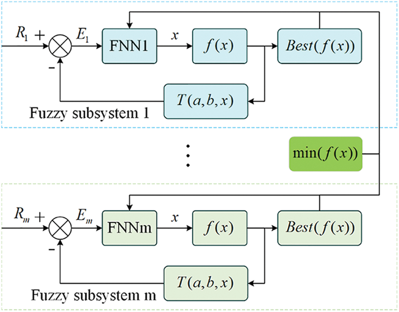
Figure 7: Multi-loop fuzzy control system block diagram

4.2 Fuzzy Particle Swarm Optimization

4.2.1 PSO Algorithm

In the standard PSO algorithm, it is assumed that in an n-dimensional problem space, there are m particles, each particle is a feasible solution to the problem to be optimized in the search space, and the optimal solution of the problem is found through cooperation and competition between particles. The process of optimization problem can be seen as a process of continuous particle update. Each particle adjusts its flight speed and direction according to Eq. (22) with the current speed, individual optimal solution and global optimal solution. The evolution equation is as follows:

{vi(t+1)=ωvi(t)+c1r1(pi−xi)+c2r2(pg−xi)xi(t+1)=xi(t)+vi(t+1)(22)

where, xi and vi represent the current position and velocity of particle i, respectively, pi and pg represent the best value searched by particle i and the best position searched by all particles in the population, respectively. r1 and r2 are random numbers in [0,1], c1 and c2 are learning factors that are constants, The ω is called the inertia weight and is generally taken as a number between 0.4 and 0.9 [24,25].

4.2.2 Fuzzy Particle Swarm Optimization Algorithm

The conventional particle swarm optimization (PSO) approach is not able to find the best solution and is prone to premature convergence. Eq. (22) can be used to get the global optimal solution of the fitness function if there are a sufficient number of particles and their initial position distributions are completely scattered. However, this process takes a long time to compute. Reducing the number of particles will solve this issue by ensuring that the finite particles’ starting locations are as far apart as possible. This work enhances particle swarm optimization, the algorithm’s local and global search capabilities, and its usage of fuzzy rules in fuzzy controllers. According to the Takagi-Sugeno fuzzy model, the fuzzy rules of the fuzzy control system in this paper are adopted as follows:

Ril: If ξ1 is Mi1l∧⋯∧ξi is Mipl then

{x1=ω0(i,l)+ω1(i,l)xi(t)x2=ω2(i,l)(xi(t)−xi(t−1))x3=ω3(i,l)r1(xibest(t)−xi(t−1))x4=ω3(i,l)r1(xallbest(t)−xi(t−1))x˙i(t)=x1+x2+x3+x4(23)

where, Ril represents the l-th fuzzy rule of the i-th fuzzy subsystem, Ni represents the number of fuzzy rules of the i-th fuzzy subsystem, p represents the number of fuzzy variables of the i-th fuzzy subsystem, xibest is the best position vector for the i-th fuzzy subsystem, xallbest is the best position vector for all fuzzy subsystems, ω0, ω1, ω2, ω3 and ω4 are the speed regulation parameters of the i-th fuzzy subsystem. Using the weighted average method to defuzzify, the global model of the i-th fuzzy subsystem can be described as:

{x1=ω0(i,l)+ω1(i,l)xi(t)x2=ω2(i,l)(xi(t)−xi(t−1))x3=ω3(i,l)r1(xibest(t)−xi(t−1))x4=ω4(i,l)r1(xallbest(t)−xi(t−1))x˙i(t)=∑lNi(x1+x2+x3+x4)hil(ξ)(24)

where, hil(ξ)=∏k=1pμMipl∑l=1Ni∏k=1pμMipl, ∑l=1Nihil(ξ)=1, μMipl is the membership function of the i-th fuzzy variable, μMipl=Ri−T(ail,bil,f), Ri is the input to subsystem i.

The design idea of membership function is expounded in combination with Fig. 8: Taking the commonly used triangular membership function as an example, the membership function width interval in Fig. 8a is denoted as ik, the width interval of the dependency function in Fig. 8b is denoated as im, if ik<im, the search range △k for the same number of membership functions is less than △m. The smaller the membership function width interval ik, the stronger the local search ability and the higher the precision of the fuzzy control system. On the contrary, the larger the membership function width interval im, the stronger the global search capability and the larger the search scope of the system. According to this idea, this paper sets n membership functions for n fuzzy control subsystems, as shown in Fig. 9. The membership function width interval of the k th fuzzy control subsystem is ik, and the membership function width interval of the m th fuzzy control subsystem is im, ik<im (m, k = 1,2, · · ·, n). In this way, the membership function width interval of each fuzzy control subsystem is different, and the control system with narrow membership function width interval has strong local search ability and high precision. The control system with wide membership function width has strong global search ability and large search range, which makes up for the defects of traditional particle swarm optimization.

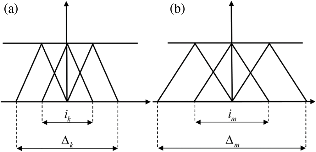
Figure 8: (a) Membership function of μMikpl (b) Membership function of μMimpl

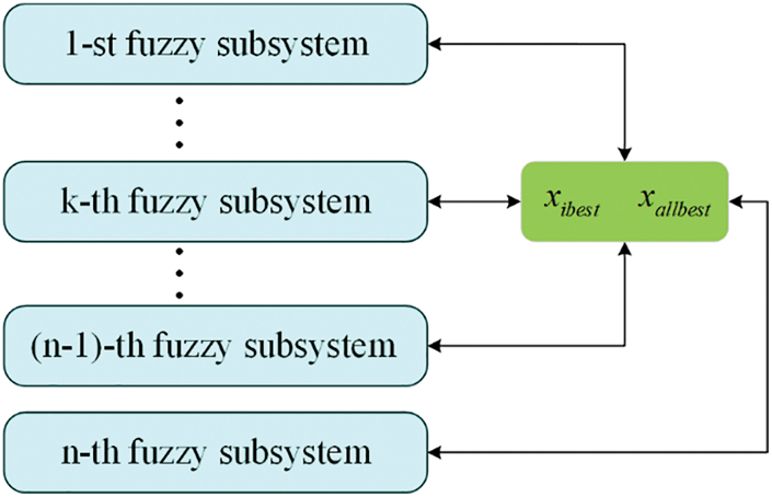
Figure 9: The relationship with all subsystems

It can be seen that for n fuzzy control subsystems, the width interval of the membership function can be changed only by setting the parameter a of the transformation function, that is, aikl<aiml, then ik<im. At this time, the setting of n fuzzy control subsystems is to set a as n row matrix. The larger the value of ak, the narrower the width interval of the membership function of the k-th sub-system, the stronger the local search ability and the higher the precision of the fuzzy control subsystem. On the contrary, the smaller the value of am, the wider the membership function of the m-th sub-system, the stronger the global search ability of the fuzzy subsystem, and the larger the search range. When a very small positive number is taken from the walk length, the discretization of Eq. (24) is described as follows:

{x0=xi(k)x1=ω0(i,l)+ω1(i,l)xi(k)x2=ω2(i,l)(xi(k)−xi(k−1))x3=ω3(i,l)r1(xibest(k)−xi(k))x4=ω4(i,l)r1(xallbest(k)−xi(k))xi(k+1)=x0+η4∑lNi(x1+x2+x3+x4)hil(ξ)(25)

here η4 is the length from the walk, a very small positive number. ω0, ω1, ω2, ω3, ω4 corrected as follows:

{ω0(i,l)=−η1(∂f(xi)/∂xi(t)+η2(xi(t)−xallbest(t)))hilω1(i,l)=−η1(∂f(xi)/∂xi(t)+η2(xi(t)−xallbest(t)))xi(t)hilω2(i,l)=−η1(∂f(xi)/∂xi(t)+η2(xi(t)−xallbest(t)))(xi(t)−xi(t−1))hilω3(i,l)=−η1(∂f(xi)/∂xi(t)+η2(xi(t)−xallbest(t)))(xallbest(t)−xi(t))hilω4(i,l)=−η1(∂f(xi)/∂xi(t)+η2(xi(t)−xallbest(t)))(xibest(t)−xi(t))hil(26)

where, i=1,2,⋯,n, l=1,2,⋯,Ni, η1, η2 are small positive numbers, n is the number of subsystems.

4.2.3 Filled Function

Fuzzy particle swarm optimization (FPSO) improves the global search ability of particle swarm optimization, but it also has the possibility of falling into local extreme points. Therefore, a filled function is constructed to make the algorithm have the ability to jump out of the local extreme point to a smaller point, so as to search for the global optimal value.

The main logic of the filled function method is that if a local minimum x1 has been found, but it is not a global minimum, construct a filled function at x1 so that the iteration point leaves the valley where x1 is located, and find a better solution for x2 (i.e., the fitness function value at x2 is smaller than the fitness function value at x1). As shown in Fig. 10, construct a function P(x), called the filled function, from a known minimum point x1 of the fitness function f(x), which takes a maximum value at x1, there is no minimum point or saddle point in any basin higher than B1 of x1, but there is a minimum point or saddle point x∗ in some basin lower than x1, then minimize f(x) with x∗ as the initial point and finds a new minimum x2, making F(x2)≤F(x1), replacing x2 with x1, repeat the process until the global minimum of f(x) is found [26,27]. Common filled functions are as follows:

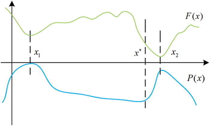
Figure 10: Filled function diagram

G(x,x1,r,ρ)=−ρ2log⁡(x+f(x))−‖x−x1‖2(27)

Q(x,x1,a)=−(f(x)−f(x1))exp⁡(a‖x−x1‖2)(28)

where, r, ρ, a are the parameters that need to be adjusted during the calculation, Eq. (27) is a two-parameter filled function, which is troublesome and time-consuming to adjust, while Eq. (28) is a single-parameter filled function, however, only when a is large, it can become a filled function at x1, because the parameter a is on the exponential, when a is large, the calculation performance is not ideal. This paper constructs a new filled function:

{P(x,x1)=−sgn(f(x)−f(x1))(‖x−x1‖/(1+‖x−x1‖))sgn(t)={1,t≥0−1,t<0(29)

the filled function is parameterless, which can save the long calculation steps and the time of adjusting parameters, so as to improve the efficiency of the algorithm.

4.3 FPSOTF Algorithm Flow

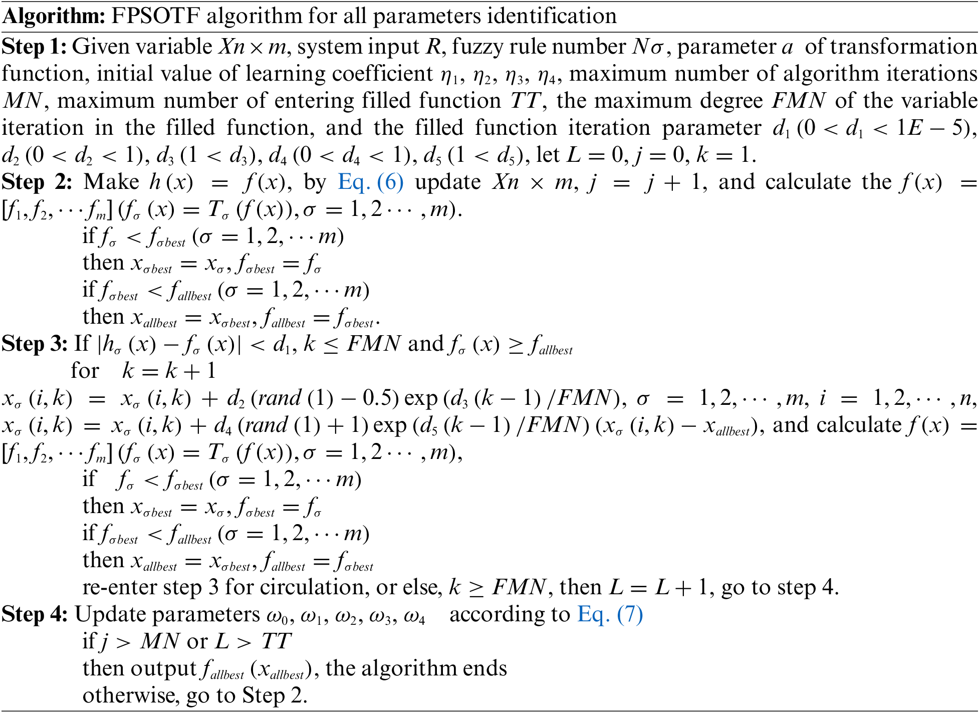
The flow of fuzzy particle swarm optimization algorithm based on filled function and transformation function (FPSOTF) is shown in Fig. 11.

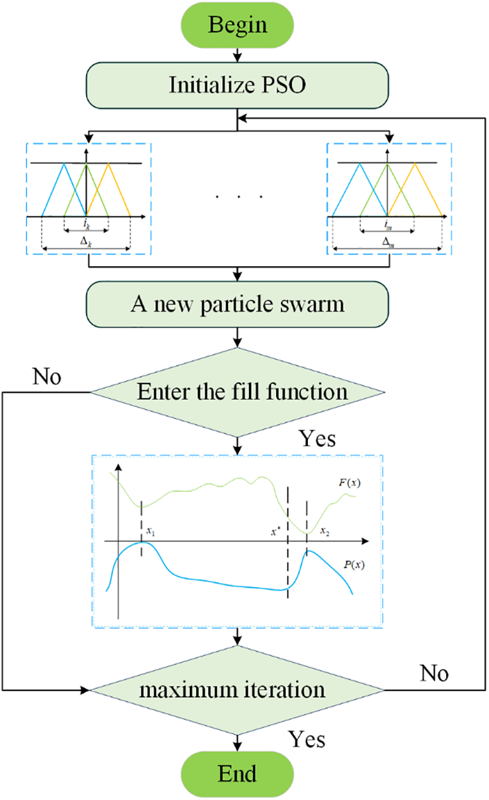
Figure 11: Flowchart of FPSO-TF algorithm

5  Simulation Results and Analysis

To parameterize PMSM in this simulation, a MATLAB/Simulink platform simulation model based on the FPSOTF is constructed. The simulation model’s parameters are configured as shown in Table 1.

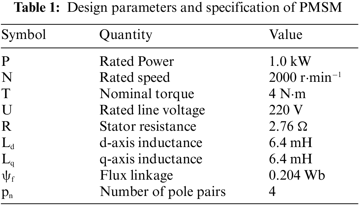
In order to make the simulation results scientific and comparable, FPOTF was compared with four algorithms, FPSO, CPSO and CFPSO, and the simulation parameters of these five algorithms were set to the same value, and the initial values of all five parameters to be identified were set in the range of (–20,20). The initial values of the five parameters to be identified differ greatly from the real values set in the simulation. In order to reduce the error caused by the randomness of the algorithm, each algorithm is independently run 100 times, and the final result is the average value of the 100 simulation results.

The simulation results are shown in Table 2.

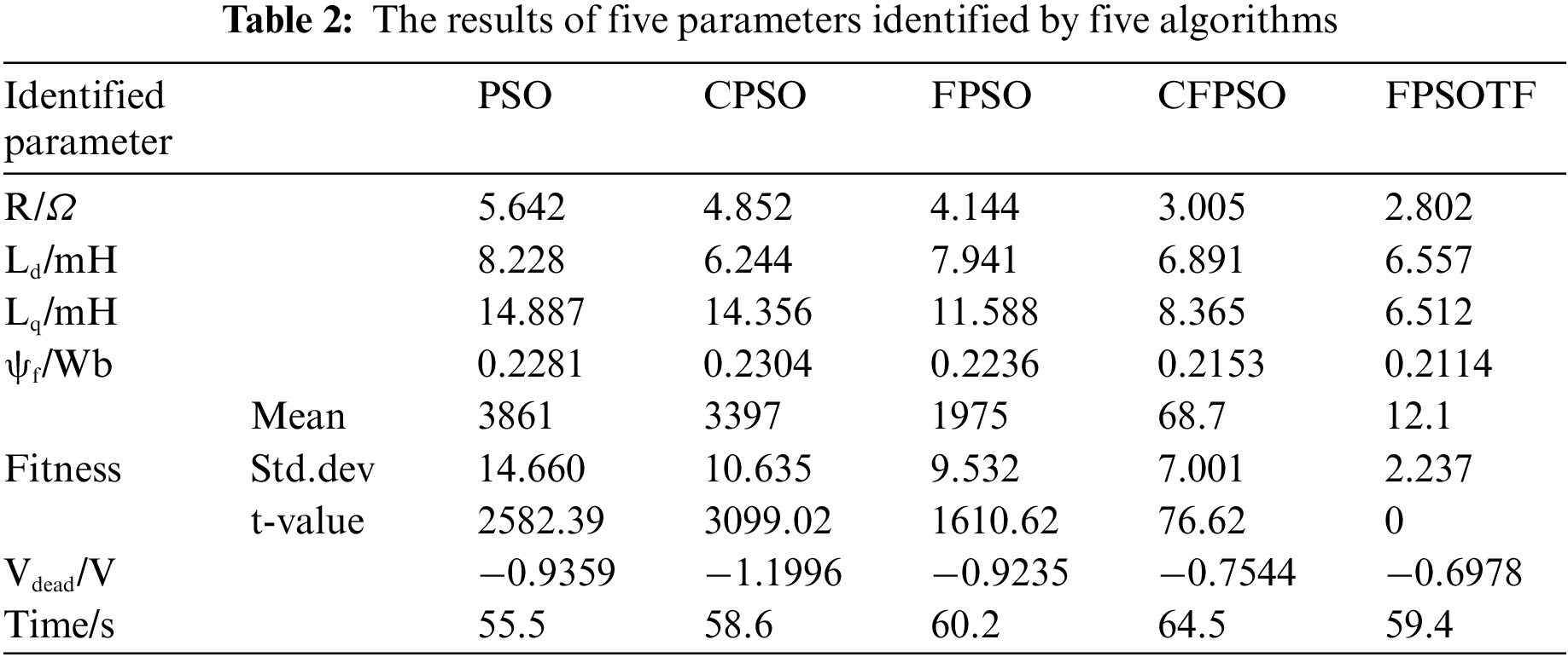
The data in Tables 2 and 1 show that, with the least amount of error and average fitness function value, the identification results of the five FPSOTF algorithm parameters are closest to the set values. Table 2’s t-value indicates that the FPSOTF in this study and the other four variation PSO algorithms all have t-values higher than 2.06, indicating that FPSOTF is significantly more effective than the other four variant PSO algorithms for PMSM multi-parameter identification. 98 percent of the time. The algorithm’s running time in Table 2 shows that, in comparison to the PSO algorithm, the FPSOTF algorithm runs longer, increasing by 7%, decreasing by 1.3%, and increasing by 1.4% when compared to the CPSO algorithm. In contrast, the CFPSO algorithm runs slower, decreasing by 8%. This demonstrates that the FPSOTF algorithm’s complexity rises when compared to the PSO algorithm but falls when compared to the FPSO and CFPSO algorithms. This demonstrates how well the FPSOTF algorithm strikes a compromise between computational complexity and balance identification accuracy. The comparison’s findings demonstrate that the FPSOTF algorithm performs better than the other methods.

Table 3 presents a comparison of the identification accuracy of PMSM parameters using the algorithm suggested in this paper with reference 7. The table shows that for stator resistance and q-axis inductance, the identification accuracy of the technique suggested in this study is higher than that of reference 7, but for d-axis inductance and flux linkage, it is marginally worse. This demonstrates that the method presented in this study has advanced to a satisfactory level; however, more research is needed to properly balance the identification accuracy across different parameters. The identification process of five parameters of PMSM by five algorithms is shown in Figs. 12–14.

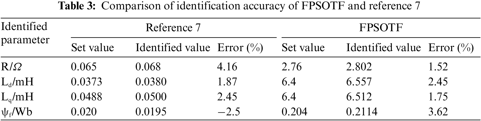
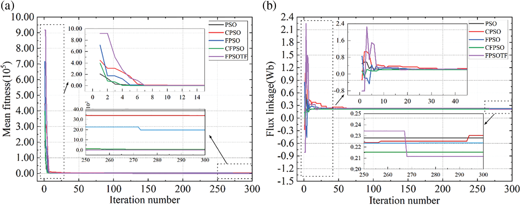
Figure 12: (a) Mean fitness value curve; (b) Flux linkage curve

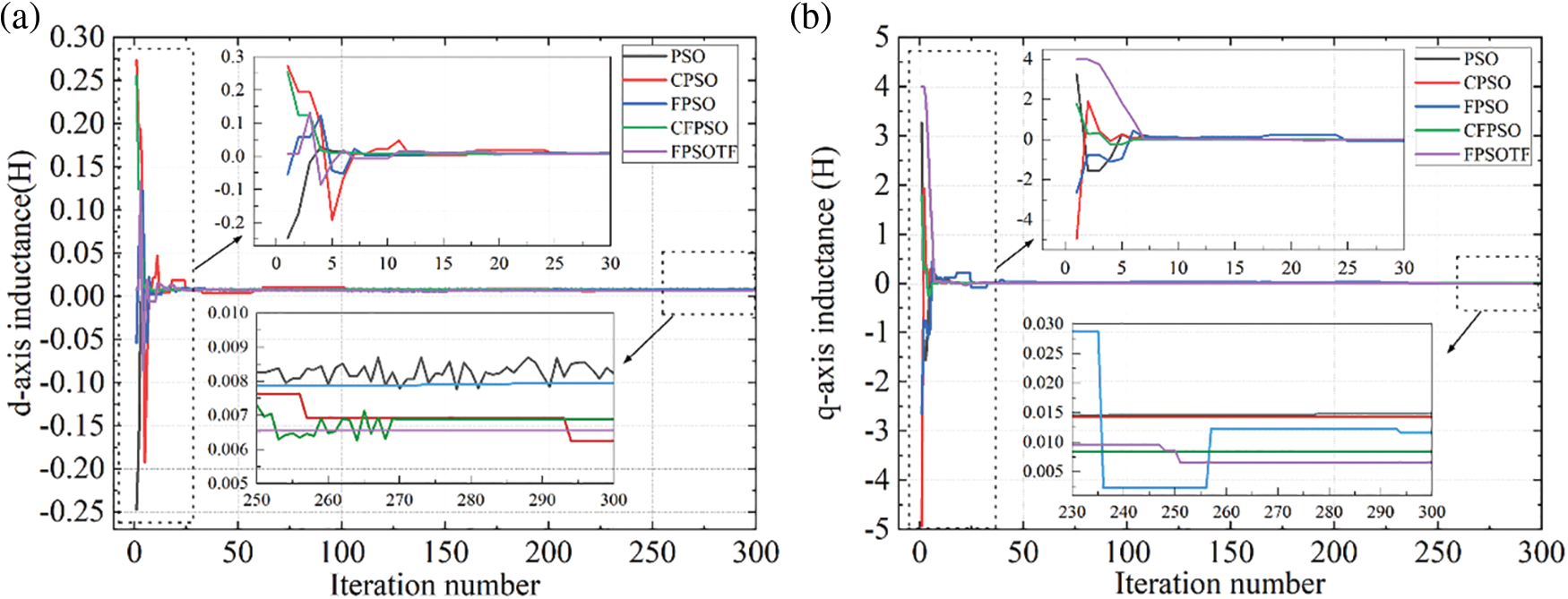
Figure 13: (a) D-axis inductance curve; (b) Q-axis inductance curve

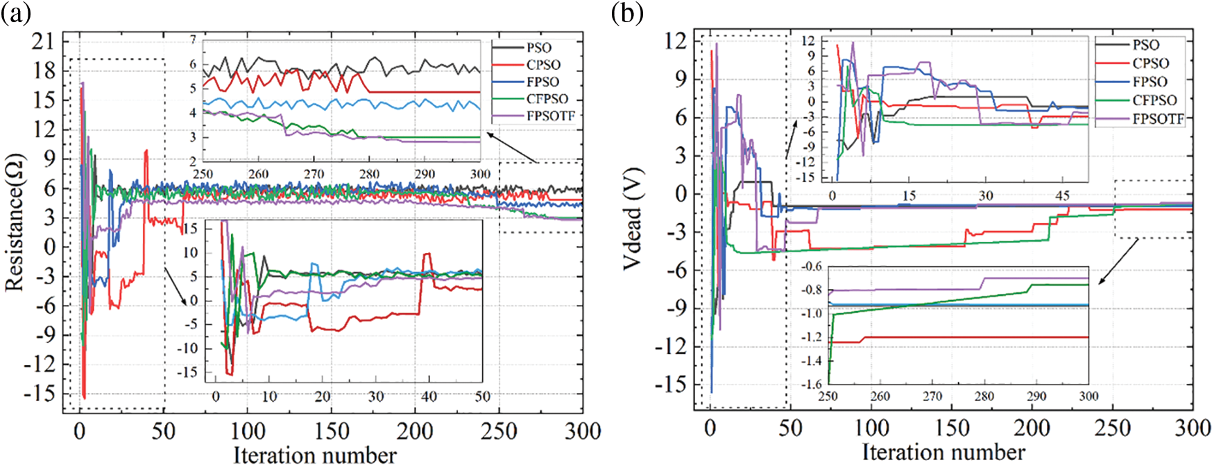
Figure 14: (a) Stator resistance curve; (b) VSI disturbance voltage curve

The mean fitness value curve in the process of calculating various algorithms is shown in Fig. 12a. The FPSOTF method suggested in this research enters the stable search phase more slowly than the other four algorithms, as seen in the figure, suggesting that the FPSOTF algorithm has superior global search capabilities. While the fitness values of CFPSO and FPSOTF are small—FPSOTF being the smallest—and thus suggest that these two algorithms have superior local searching ability, the fitness values of PSO, CPSO, and FPSO are always large, suggesting that these three algorithms are trapped in local optimal solutions.The flux linkage convergence curve for the five algorithms’ computation is shown in Fig. 12b. The figure shows that all five algorithms have essentially finished the global search in less than 50 iterations, and there is little variation in the convergence speed of the algorithms. Each algorithm has reached the stable search phase after 50 iterations, and the chart shows that all five algorithms have reached the local search phase after 270 iterations. The other three algorithms’ poor search accuracy suggests that they are stuck in the local optimal solution and are unable to escape, whereas CFPSO and FPSOTF exhibit excellent search accuracy. According to the final outcome, FPFOTF has the best search accuracy.

Fig. 13 is the convergence curve of the d/q axis inductance. It can be seen from the figure that all five algorithms have completed convergence within 30 iterations, that is, global search has been realized, and the five algorithms can complete global search in a relatively short time, indicating that inductance is an easy parameter to identify, and that the calculation speed of the five algorithms in the early search process is basically the same. However, in the refined search process after 270 iterations, only CFPSO and FPSOTF have better search accuracy, among which FPSOTF algorithm can better stabilize near the set value, which indicates that the FPSOTF algorithm has better search ability compared with other algorithms.

The convergence curve for stator resistance during the five algorithms’ computation process is shown in Fig. 14a. The figure shows that the resistance has not converged well and fluctuates significantly over the entire computation procedure, suggesting that the resistance is a difficult-to-identify quantity. Different algorithms can do fine search more effectively after 280 iterations. Nevertheless, within a specific numerical range, the three algorithms—PSO, CPSO, and FPSO—still fail to stabilize the identification findings. The algorithm’s search capacity is demonstrated by the nearly ideal final search results of CFPSO and FPSOTF, as well as the identification results of FPSOTF that are closest to the set value.

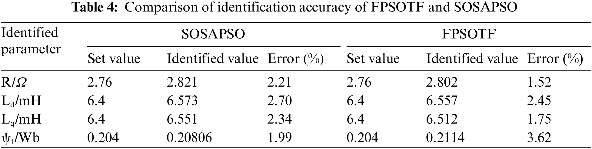
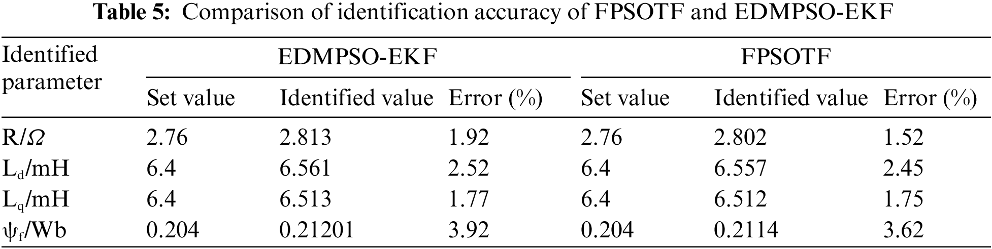
The disrupted voltage curve of VSI is displayed in Fig. 14b. The figure illustrates how this parameter’s convergence process takes a while. The fact that the CPSO and CFPSO algorithms needed 280 iterations to do fine searches suggests that they are not very good at conducting global searches to find this parameter. The FPSOTF algorithm’s identification result is the one that comes the closest to the set value in the final result. The FPSOTF method outperforms the other four algorithms in terms of calculation performance and has good global and local search capabilities throughout the identification process. At present, in the recent research, two improved PSO algorithms are proposed in reference 29 and 30, respectively, SOSAPSO (a novel multi-strategy self-optimizing simulated annealing particle swarm optimization) and EDMPSO-EKF (mean particle swarm optimization with extreme disturbance combined with extended Kalman filter), The algorithm proposed in this paper is compared with these two algorithms, and the results are as follows.

Tables 4 and 5 show that, in comparison to the FPSOTF algorithm, the SOSAPSO algorithm’s identification errors for flux linkage are smaller, but the algorithm’s identification errors for stator resistance, d-axis inductance, and q-axis inductance are marginally higher. For all four parameters, the MDEPSO-EKF algorithm’s identification errors are larger than the FPSOTF algorithm’s. Overall, the four parameters’ identification accuracy is higher for the FPSOTF method, suggesting that the algorithm presented in this study is more capable of identification. On the other hand, the comparison with the SOSAPSO method reveals that the FPSOTF algorithm has a significant inaccuracy in flux linkage identification, so the future research should balance the identification accuracy of the four parameters.

Due to the substantial nonlinearity of the PMSM model and the abundance of local extremum points in the fitness function, the technique exhibits significant fluctuation or non-convergence in parameter identification of PMSM. This makes finding the optimal solution difficult for algorithms with limited processing power. The FPSOTF algorithm outperforms the other algorithms in terms of identification accuracy, as demonstrated by the identification procedure and results. Additionally, the data in the table demonstrates that the FPSOTF method has the lowest average fitness value and an identification value that is closer to the design value, suggesting that the algorithm is better and has strong robustness and convergence.

6  Conclusion and Future Directions

The study develops a thorough mathematical model of PMSM that takes into consideration the voltage source-inverter’s (VSI) nonlinearity and how it affects parameter identification. Furthermore, by combining FPSO with the transformation function and filled function, a brand-new algorithm known as FPSOTF is presented. The filled function improves PSO's local search capabilities, while the transformation function makes the process of finding fitness functions less difficult. Consequently, five parameters are correctly identified by this algorithm. This approach provides strong anti-interference ability and computing performance during parameter identification of PMSM, as demonstrated by a comparative comparison with four other algorithms. Because of their powerful nonlinear optimization capabilities, artificial intelligence algorithms have drawn a lot of attention. However, these algorithms also have significant computational and data processing overhead. Consequently, more study is required to decrease the computational burden of artificial intelligence algorithms and increase their identification accuracy.

Acknowledgement: We are grateful for the valuable comments provided by the anonymous reviewers, which have helped us to improve the content of this paper and make it even better.

Funding Statement: This work was supported in part by the Natural Science Foundation of China under Grant 52077027, and in part by the Liaoning Province Science and Technology Major Project No. 2020JH1/10100020.

Author Contributions: The authors confirm contribution to the paper as follows: Study conception and design: Shuai Zhou and Dazhi Wang; data collection: Yongliang Ni, Keling Song and Yanming Li; analysis and interpretation of results: Shuai Zhou; draft manuscript preparation: Shuai Zhou. All authors reviewed the results and approved the final version of the manuscript.

Availability of Data and Materials: Data not available due to [ethical/legal/commercial] restrictions. Due to the nature of this research, participants of this study did not agree for their data to be shared publicly, so supporting data is not available.

Conflicts of Interest: The authors declare that they have no known competing financial interests or personal relationships that could have appeared to influence the work reported in this paper.

References

1. Z. Wang, J. Chai, X. Xiang, X. Sun, and H. Lu, “A novel online parameter identification algorithm designed for deadbeat current control of the permanent-magnet synchronous motor,” IEEE Trans. Ind. Applicat., vol. 58, no. 2, pp. 2029–2041, Apr. 2022. doi: 10.1109/TIA.2021.3136807. [Google Scholar] [CrossRef]

2. Z. Q. Zhu, D. Liang, and K. Liu, “Online parameter estimation for permanent magnet synchronous machines: An overview,” IEEE Access, vol. 9, pp. 59059–59084, Oct. 2021. doi: 10.1109/ACCESS.2021.3072959. [Google Scholar] [CrossRef]

3. Y. L. Yu, X. Y. Huang, and Z. K. Li, “Overall electrical parameters identification for IPMSMs using current derivative to avoid rank deficiency,” IEEE Trans. Ind. Electron., vol. 70, no. 7, pp. 7515–7520, Jul. 2023. doi: 10.1109/TIE.2022.3203751. [Google Scholar] [CrossRef]

4. W. Feng, W. J. Zhang, and S. D. Huang, “A novel parameter estimation method for PMSM by using chaotic particle swarm optimization with dynamic self-optimization,” IEEE Trans. Veh. Technol., vol. 72, no. 7, pp. 8424–8432, Jul. 2023. doi: 10.1109/TVT.2023.3247729. [Google Scholar] [CrossRef]

5. Y. L. Yu et al., “Full parameter estimation for permanent magnet synchronous motors,” IEEE Trans. Ind. Electron., vol. 69, no. 5, pp. 4376–4386, May 2022. doi: 10.1109/TIE.2021.3078391. [Google Scholar] [CrossRef]

6. S. A. Odhano, P. Pescetto, H. A. A. Awan, M. Hinkkanen, G. Pellegrino and R. Bojoi, “Parameter identification and self-commissioning in AC motor drives: A technology status review,” IEEE Trans. Power Electron., vol. 4, no. 34, pp. 3603–3614, Apr. 2019. [Google Scholar]

7. Z. W. Wang et al., “UKF-based parameter estimation and identification for permanent magnet synchronous motor,” Front. Energy Res., vol. 10, no. 1, pp. 855649–855658, 2022. [Google Scholar]

8. S. Xiao and A. Griffo, “Online thermal parameter identification for permanent magnet synchronous machines,” IET Electr. Power Appl., vol. 14, no. 12, pp. 2340–2347, 2020. [Google Scholar]

9. M. Koc and O. E. Ozciflikci, “Precise torque control for interior mounted permanent magnet synchronous motors with recursive least squares algorithm based parameter estimations,” Eng. Sci. Technol. Int. J., vol. 34, no. 1, pp. 101087–101093, 2022. [Google Scholar]

10. H. Yu, J. Wang, and Z. Xin, “Model predictive control for PMSM based on discrete space vector modulation with RLS parameter identification,” Energies, vol. 15, no. 11, pp. 4041–4057, 2022. [Google Scholar]

11. C. Y. Yang, L. C. Bu, and B. Chen, “Energy modeling and online parameter identification for permanent magnet synchronous motor driven belt conveyors,” Measurement, vol. 178, no. 1, pp. 109342–109350, 2021. [Google Scholar]

12. X. Qi, C. Sheng, Y. Guo, T. Su, and H. Wang, “Parameter identification of a permanent magnet synchronous motor based on the model reference adaptive system with improved active disturbance rejection control adaptive law,” Appl. Sci., vol. 13, no. 21, pp. 12076–12090, Jan. 2023. doi: 10.3390/app132112076. [Google Scholar] [CrossRef]

13. J. She, L. Wu, C. K. Zhang, Z. T. Liu, and Y. H. Xiong, “Identification of moment of inertia for PMSM using improved modelreference adaptive system,” Int. J. Control Autom. Syst., vol. 20, no. 1, pp. 13–23, 2022. doi: 10.1007/s12555-020-0549-8. [Google Scholar] [CrossRef]

14. Z. H. Liu, H. L. Wei, X. H. Li, K. Liu, and Q. C. Zhong, “Global identification of electrical and mechanical parameters in PMSM drive based on dynamic self-learning PSO,” IEEE Trans. Power Electron., vol. 33, no. 12, pp. 10858–10871, Dec. 2018. doi: 10.1109/TPEL.2018.2801331. [Google Scholar] [CrossRef]

15. R. A. El-Wanis and M. A. Hamida, “Parameter estimation of permanent magnet synchronous machines using particle swarm optimization algorithm,” RRST-EE, vol. 67, no. 4, pp. 377–382, Dec. 2022. [Google Scholar]

16. J. He and Z. H. Liu, “Estimation of stator resistance and rotor flux linkage in SPMSM using CLPSO with opposition-based-learning strategy,” J. Control Sci. Eng., vol. 2016, no. 5781467, 2016. doi: 10.1155/2016/5781467. [Google Scholar] [CrossRef]

17. G. Lin, J. Zhang, and Z. Liu, “Parameter identification of PMSM using immune clonal selection differential evolution algorithm,” Math. Probl. Eng., vol. 2014, no. 6, pp. 1–10, 2014. doi: 10.1155/2014/160685. [Google Scholar] [CrossRef]

18. K. Liu and Z. Q. Zhu, “Position-offset-based parameter estimation using the adaline NN for condition monitoring of permanent-magnet synchronous machines,” IEEE Trans. Ind. Electron., vol. 62, no. 4, pp. 2372–2383, Apr. 2015. doi: 10.1109/TIE.2014.2360145. [Google Scholar] [CrossRef]

19. W. Feng, W. Zhang, and S. Huang, “A novel parameter estimation method for PMSM by using chaotic particle swarm optimization with dynamic self-optimization,” IEEE Trans. Veh. Technol., vol. 72, no. 7, pp. 8424–8432, Jul. 2023. doi: 10.1109/TVT.2023.3247729. [Google Scholar] [CrossRef]

20. D. D. Wen et al., “A novel multi-strategy self-optimizing SAPSO algorithm for PMSM parameter identification,” IET Power Electron., vol. 16, no. 2, pp. 305–319, Aug. 2023. doi: 10.1049/pel2.12385. [Google Scholar] [CrossRef]

21. Q. Xiao, K. Liao, C. Shi, and Y. Zhang, “Parameter identification of direct-drive permanent magnet synchronous generator based on EDMPSO-EKF,” IET Renew. Power Gen., vol. 16, no. 5, pp. 1073–1086, Jan. 2022. doi: 10.1049/rpg2.12415. [Google Scholar] [CrossRef]

22. G. Su, P. Wang, Y. Guo, G. Cheng, S. Wang and D. Zhao, “Multiparameter identification of permanent magnet synchronous motor based on model reference adaptive system—simulated annealing particle swarm optimization algorithm,” Electronics, vol. 11, no. 1, pp. 159–176, Jan. 2022. doi: 10.3390/electronics11010159. [Google Scholar] [CrossRef]

23. M. A. Ahandani, J. Abbasfam, and H. Kharrati, “Parameter identification of permanent magnet synchronous motors using quasi-opposition-based particle swarm optimization and hybrid chaotic particle swarm optimization algorithms,” Appl. Intell., vol. 52, no. 11, pp. 13082–13096, Jan. 2022. doi: 10.1007/s10489-022-03223-x. [Google Scholar] [CrossRef]

24. J. Kennedy and R. Eberhart, “Particle swarm optimization,” in Proc. ICNN’95-Int. Conf. Neural Netw., Perth, WA, Australia, 1995, pp. 1942–1948. [Google Scholar]

25. Z. H. Zhan, J. Zhang, Y. Li, and Y. H. Shi, “Orthogonal learning particle swarm optimization,” IEEE Trans. Evol. Computat., vol. 15, no. 6, pp. 832–847, Dec. 2011. doi: 10.1109/TEVC.2010.2052054. [Google Scholar] [CrossRef]

26. A. I. Ahmed, “A new parameter free filled function for solving unconstrained global optimization problems,” Int. J. Comput. Math., vol. 98, no. 1, pp. 106–119, Jan. 2021. doi: 10.1080/00207160.2020.1731484. [Google Scholar] [CrossRef]

27. A. Sahiner, T. Ermis, and M. W. Awan, “A new filled function for global optimization,” Analele Stiintifice ale Universitatii Ovidius Constanta, Seria Matematica, vol. 31, no. 3, pp. 207–220, Sep. 2023. [Google Scholar]