Fusion of Spiral Convolution-LSTM for Intrusion Detection Modeling

1  Related Work

Deep learning technology has been changing day by day, at 2017, the researcher used convolutional neural network (CNN) [1] to detect abnormal behaviors in network traffic, at that time, the researchers found that CNN could be more effective than the traditional intrusion detection methods, and CNN can be processed in a large amount of spontaneous data, This study provides a good demonstration for the application of machine learning models and even deep learning models in the field of intrusion detection.

Traditional machine learning methods such as support vector machine [2], correlation vector machine [3], Adaboost [4], and other algorithms, in the face of the current new cyber-attacks and high-dimensional data environment, have been unable to extract effective information from the dataset in a good way, which in turn leads to poor model accuracy.

In addition, there is also a researcher Yin et al. [5] proposed a deep learning approach for intrusion detection using Recurrent Neural Networks (RNN), the researcher compared the performance of his model for classification in binary as well as multiclassification scenarios with other models such as Artificial Neural Networks (ANNs), Random Forests and so on. The comparison led to the conclusion that recurrent neural networks are well-suited for building high-precision classification models.

There are also some researchers found the imbalance problem of some datasets, Wang et al. [6] used the improved intrusion detection model using the residual network, which firstly converted the original dataset to grayscale images and then added the attention mechanism module from the second to the fifth layer of the residual network (ResNet) structure, to construct the residual attention network algorithm, to learn more key features of the anomalous traffic. To address the class imbalance in the dataset, an improved focus loss function is used instead of the cross-entropy loss function to identify small class attacks in the dataset, and the paper indicates that its method has improved performance compared to the original cross-entropy loss function model.

Some researchers have focused on the dataset itself to do research, and dataset preprocessing methods have proliferated. Panigrahi proposed an improved version of the random sampling mechanism, which researchers named Supervised Relative Random Sampling (SRRS) [7], which is commonly used in the preprocessing stage of deep learning models to generate balanced samples from imbalanced datasets. Kasongo et al. [8] used a downscaled compression of the feature method to process the dataset before training the model and also achieved good results. Takahashi et al. [9] uses a new data enhancement technique called Randomized Image Cropping and Patching (RICAP), which randomly crops four images and patches, at last them to create new training images. Abdel-Nasser et al. [10] used a long and short-term memory network (LSTM) to predict photovoltaic power generation. The researcher said that due to the cyclic architecture and storage unit of LSTM, the LSTM network can model the time change of photovoltaic power output. Compared with other methods, using LSTM further reduces the prediction error.

There are many deep learning algorithms, traditional deep learning algorithms such as CNN, RNN, Deep Neural Network (DNN), Gate Recurrent Unit (GRU), etc., which are commonplace in the field of intrusion detection. However, some non-traditional deep learning methods shine in other scientific research today such as Spiral convolution [11], Deformable Convolutional Neural Networks [12], Spatio-temporal convolutional neural networks [13], and so on. However, these methods have not yet been used by researchers in the field of intrusion detection.

With the development of deep learning nowadays, numerous researchers have applied it to the field of intrusion detection. In this paper, after reviewing numerous articles in the field, we found that the current deep-learning intrusion detection model still has the following problems:

(1)   The preprocessing of the original dataset is slightly cumbersome, ignoring the model’s perception of the dataset, and putting the cart before the horse;

(2)   Model training is computationally intensive and model convergence is slow;

(3)   Poor model generalization ability, most models have high accuracy for one dataset and poor results in other datasets.

The contribution of this paper will focus on the above problems for research.

In this paper, to address the aforementioned issues, non-traditional convolutional neural network Spiral convolution is used to carry out preliminary feature extraction on the dataset and to remove the low correlation features and redundant information the maximum pooling layer is introduced to reduce the number of model parameters and accelerate the model convergence. At the same time, a multilayer LSTM is used to retain the temporal features, and finally, the Softmax classifier is used to classify the output.

The following is an overview of the subsequent structure of this article: Section 2 provides a detailed explanation of the model construction process and the methods used. In Section 3, a comprehensive evaluation of the proposed method was conducted through comparative experiments and ablation experiments. Finally, an objective summary is provided in Section 4 to conclude the entire article.

2  SCL Model Construction

The structure of the spiral convolutional intrusion detection model in this paper mainly has the spiral convolutional layer, pooling layer, LSTM layer, and other layers. The picture in Fig. 1 shows the model structure diagram.

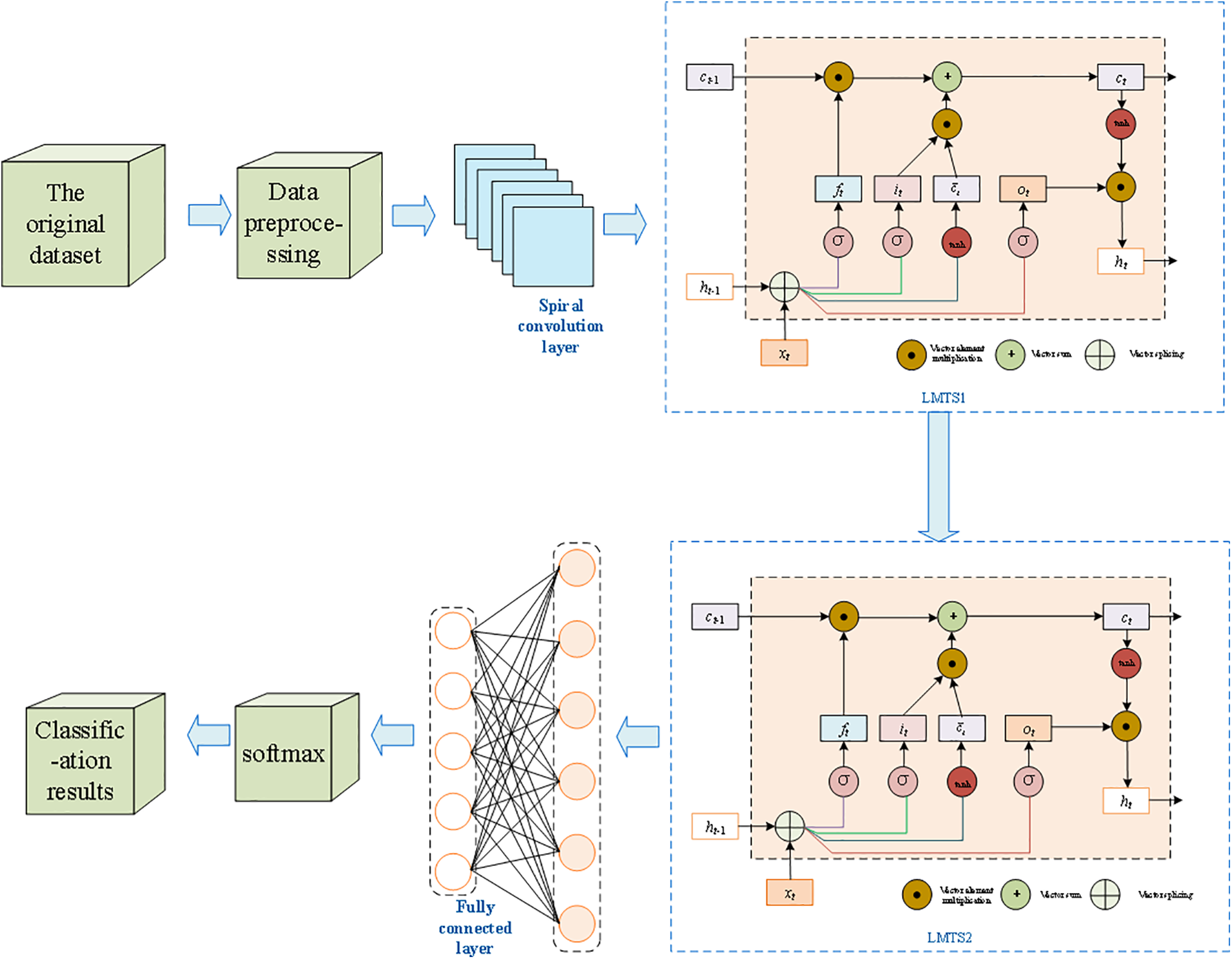
Figure 1: SCL model architecture diagram

2.1 Raw Dataset and Preprocessing

2.1.1 Raw Dataset

This study will use the NSL-KDD [14] dataset to study the problem of intrusion detection classification. This dataset is widely used for the performance evaluation of intrusion detection systems (IDS), and it is derived from the KDD Cup 99 dataset, one of the most commonly used datasets in this field. However, there are some disadvantages in the KDD Cup 99 dataset, such as data redundancy, so later researchers developed a new NSL-KDD dataset based on the original dataset. In the new NSL-KDD dataset, there are four different attack types, which are: Denial of service (DoS), detection, user to root (U2R), and remote to local (R2L).

The dataset contains 43 features, 41 of which are network traffic inputs, and the remaining two features are labels representing network packets (attack vs. normal) and scores (attack severity). As mentioned earlier, there are four types of attacks in the data set, namely Remote to Local (R2L), Probe, User to Root (U2R), and Denial of Service (DoS) attacks. Among them, the DoS attack is a powerful attack mode that hackers use to make the system unavailable to the end user, and among the four attack modes, the DoS attack is more common and more numerous than probing or U2R. Three types of attacks, R2L, probe, and U2R, attempt to infiltrate a system without being detected. In this dataset, the four attack types DoS, Probe, U2R, and R2L are divided into 11, 6, 7, and 15 subcategories, respectively.

This paper also uses the high-dimensional dataset to validate the model generalization capability.

2.1.2 Data Preprocessing

Data preprocessing means preparing the data so that a computer can understand it better. This helps to make the data better and easier to work with in the future. Some of the information in the NSL-KDD dataset is stored as string data type. This paper uses one-hot encoding to change non-numerical values into numbers because the algorithm only works with numerical types.

Numerical normalization is an important step in the data preprocessing process, Scaling the values in the dataset to a universal scale, if this operation is not carried out, it will make the model difficult to converge in the subsequent training, We use a method called Min-Max Normalize to do this. The formula is like this:

Xi=Xi−XminXmax−Xmin(1)

2.2 Spiral Convolutional Layers

2.2.1 Spiral Sequence

Spiral sequence: Is a sequence of data generated by arranging the data in a spiral order, this transformation process is called spiralization. Spiralizing data can improve computational efficiency and greatly accelerate the convergence speed and training time of the model. For example, in traditional computer vision, data spiralization can be used to increase the speed of image processing. In graphics, data spiralization can improve the rendering speed of 3D models.

In this paper, the steps of spiral sequence transformation for one-dimensional data are as follows:

(1)   First calculate the length of the input data

(2)   Create a continuous indexed array using the range () function

(3)   Then use the enumerate () function to create an index array containing the data index and the data value

(4)   Use index data to convert input data into spiral data

(5)   The spiral sequence is obtained

2.2.2 Spiral Convolution

Spiral convolution is a kind of non-traditional convolution operation, which firstly helices the data and then computes the convolution. Spiral convolution improves the computational efficiency of convolution operation and can be used to deal with data with special structures.

Spiral convolution works by spiralizing the data and then using the convolution kernel to slide over the spiral sequence to perform the convolution calculation.

2.2.3 One-Dimensional Spiral Convolution

Three-dimensional spiral convolution is a variant of the convolution operation that can be used to process three-dimensional data with a spiral structure. The convolution kernel of 3D spiral convolution has a spiral shape and can be convolved along three dimensions (spatial, temporal, and frequency dimensions).

When performing one-dimensional spiral convolution operations, first establish a spiral index matrix Z, assuming that the model inputs a sequence X with a length of N and a spiral convolution kernel of Y. Arrange the input sequence according to the index matrix Z to obtain the input sequence Xz for spiral convolution. Then, the new input sequence is convolved with the convolution kernel Y to obtain the output P. The formula can be expressed as:

P=Y∗Xz(2)

Similar to the idea of 3D spiral convolution, the convolution kernel of 1D spiral convolution has a spiral shape and can be convolved along one dimension of the sequence data. To reduce the length of the output sequence while retaining the main features, a pooling layer can also be added after the one-dimensional spiral convolution layer, and after obtaining the features extracted from the spiral convolution layer, a fully connected layer is used to complete the classification of the features.

In conclusion, the backbone network of one-dimensional spiral convolution and traditional convolutional neural network also contains a convolutional layer, pooling layer, and fully connected layer, respectively, to realize the automatic extraction, degradation, and identification of input data features. In addition, to prevent the model from overfitting, a weight regularization term or a dropout layer can also be added to the network.

2.3 Maxpool Layer and Batch Normalization Layer

The most intuitive use of a pooling layer for a model is to reduce the number of parameters and remove redundant information. Of course, the pooling layer can also compress the features, simplify the network complexity, reduce memory consumption, and so on. The second role that researchers tend to overlook is that the pooling layer can alleviate the over-sensitivity of the convolutional layer to position, which can also be referred to as feature invariance.

The batch normalization layer can constantly adjust the intermediate outputs of the neural network while the model is being trained, thus making the output values of the entire neural network more stable from layer to layer.

2.4 LSTM Layers and Fully Connected Layers

2.4.1 LSTM Network

In traditional neural networks, most models do not focus on what information is available from an operation in the previous moment to be used in the next moment but only focus on the operation in the current moment at a time. For example, if we want to categorize events that occur at each moment in a video, it is easy to categorize events that occur at the current moment if we know information about events that occurred the moment before that video. In fact, traditional neural networks do not have memory functions (such as CNNS, DNNS, etc.), so they do not use information that has already appeared in the past when classifying or predicting events that occur at every moment. This is why we need the LSTM network, which can derive the current output from the current input and the output of the previous moment. In layman’s terms, this means that it can use information learned in the previous moment to learn in the present moment.

As for choosing LSTM over RNN, the reason is that LSTM has two advantages over traditional RNN:

(1)   LSTM can alleviate the problem of gradient vanishing and explosion in traditional deep learning to some extent;

(2)   When processing time series data, LSTM’s memory unit can effectively remember the long-term dependent information, thus realizing more accurate data prediction.

The problem of gradient vanishing in RNN is caused by the fact that the gradient is dominated by the gradient in the near distance while the gradient in the far distance is ignored, and this problem also hinders the learning of RNN on long sequence data. Both LSTM and GRU select the information of the previous nodes by adding various gating units, which can alleviate the problem of gradient vanishing to a certain extent, but this problem still exists for the long sequences. problem still exists for long sequences. The LSTM structure is shown in Fig. 2.

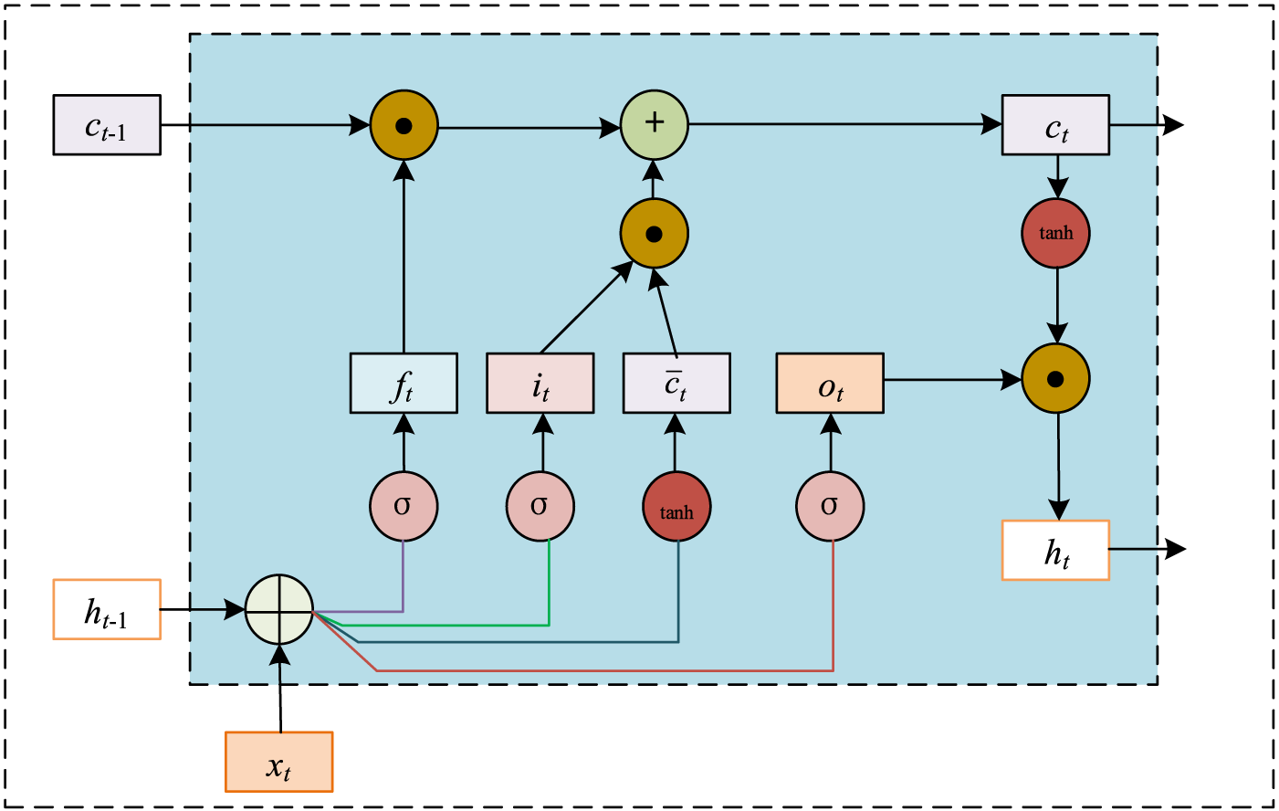
Figure 2: LSTM structure

In the figure, xt is the input at moment t, ht−1 is the output at moment t−1, and ht is the output at moment t. The most important advancement of the LSTM network is the introduction of a gating mechanism to solve the problem of gradient dispersion or vanishing. The gating mechanisms are the forget gate ft, the input gate it and the output gate ot.

The forget gate determines which information in the output memory cell ct−1 at the moment t−1 will be forgotten, and the operation is shown as follows:

ft=σ(Wxfxt+Whfht−1+bf)(3)

where bf denotes the deviation of the forget gate, σ represents the activation function sigmoid, and Wxf and Whf denote the weights of xt and ht−1 in the forget gate, respectively.

The role of input gate it is to extract the information at moment t, as well as to filter and evaluate this information, the calculation process is shown below. Where, Wxi, Whi, Wxg, Whg denote the weights of the current state. gt denotes the cell state update value, bi denotes the bias of the input gate, bg denotes the bias of gt, ct denotes the memory cell at the moment of t, tanh denotes the activation function.

it=σ(Wxixt+Whiht−1+bi)(4)

gt=tan⁡h(Wxgxt+Whght−1+bg)(5)

ct=ct−1⋅ft+gt⋅it(6)

The output gate outputs the output ht at moment t, which is calculated as shown below. Where Wo denotes the weight of the output gate and bo denotes thedeviation of the output gate.

ot=σ(Wo[xt,ht−1]+bo)(7)

mt=tanh⁡(ct)(8)

ht=ot⋅mt(9)

LSTM networks are controlled by these three gates, thus selectively storing and forgetting and thus better handling long-term dependencies.

In this paper, a two-layer LSTM network is used instead of a two-layer structure, because I found that BiLSTM is almost indistinguishable from LSTM when dealing with time series problems. The computational complexity is high, and the training time for a single epoch is long.

The reason for using a two-layer LSTM instead of a one-layer LSTM is that a two-layer LSTM can extract a more abstract, high-level feature representation. The first layer LSTM takes the information from the input sequence and provides it as richer input to the second layer LSTM, which helps the model to better capture the features in the input sequence. In this paper, time series data are compressed by stacking multi-layer LSTM, and its ability to learn long-term sequences will be greatly improved. However, the number of stacked layers should not be too many, the increase in the number of layers will lead to the slowing down of the model update iteration and the decrease of the convergence effect, and it will also make the time overhead and memory overhead grow exponentially during the training process, which will easily lead to the disappearance of the gradient and other problems.

2.4.2 Fully Connected Layer

The fully connected layer, which is typically employed as the final layer of the entire neural network model and is frequently used for classification and prediction, maps the input features to the output results. The fully connected layer’s output result can be thought of as a nonlinear transformation of the input features, mapping the input feature space to the output result space and enabling the model’s complexity and nonlinear fitting capabilities.

This paper adds a fully connected layer to the tail of the model, and sets the number of nodes in the fully connected layer based on the number of categorized categories. The predicted probability of each category is then represented by a probability distribution that is created using the softmax activation function. Fig. 3 displays the model’s overall flowchart.

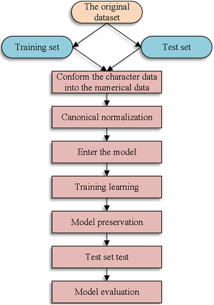
Figure 3: Overall flow chart of the model

3  Experimental Evaluation and Optimization of Result Analysis

3.1 Experimental Evaluation Index

This paper is a five-classification experiment on NSL-KDD dataset, to verify the performance of the intrusion detection model, accuracy rate (AR), precision rate (PR), recall rate (RR), and F1 score will be used to evaluate the model. The formula is shown below:

Accuracy=TP+TNTP+FN+FP+TN(10)

Precision=TPTP+FP(11)

Recall=TPTP+FN(12)

F1−score=2∗PR∗RRPR+RR(13)

where: TP denotes correctly detected attack data; FP denotes incorrectly detected normal data; TN denotes correctly detected normal data; FN denotes incorrectly detected attack data.

ROC curve: This evaluation metric was first applied in the field of radar, and it was used as an indicator to evaluate the reliability of radar during World War II. Nowadays the ROC curve has been widely used in medicine and deep learning because of its intuitive visualization. Simply put, in the curve, the horizontal axis of the coordinate system represents the false positive rate, and the vertical axis represents the true positive rate. The formula is as follows:

FPR=TPTP+FP(14)

TPR=FPFP+TN(15)

A larger area under the curve in the ROC plot indicates better model performance.

3.2 Result Analysis and Optimization

3.2.1 Result Analysis

The NSL-KDD dataset and the UNSWNB-15 [15] dataset, two significant benchmark datasets in the field of network intrusion detection, serve as the basis for the experimental data used in this research. They all have a sizable amount of data on network traffic, which includes both regular and diverse attack traffic. Models for intrusion detection can be trained and assessed using them.

The setting of hyperparameters during the experimental process usually needs to be determined through repeated experiments. After conducting a large number of experiments in this paper, the optimal parameter setting of the model was obtained.

Best hyperparameter settings used in this paper: The optimizer adopts Adam, the learning rate is set to 0.001, the batch size is set to 256, and the loss function adopts the category cross-entropy, spiral convolution kernels is set 64, layer 2 long short-term memory network settings 64, layer 2 long short-term memory network settings 128.

In order to test the effect of different numbers of spiral convolution kernels on model performance, repeated experiments were conducted using different numbers of convolution kernels. The experimental results are shown in Table 1.

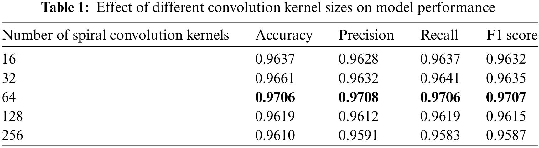
The table shows that the model achieved the best performance with the convolution kernel set to 64.

The model classification confusion matrix is shown in Fig. 4. The numbers in the squares diagonally from the top left to the bottom right represent the number of correctly classified models. The numbers in the other squares represent the number of errors in the model classification. It can be seen that the model did not perform well in dealing with a few classes in imbalanced datasets. But on the whole, the model performs well. In the future, we will consider using data augmentation methods to optimize such problems.

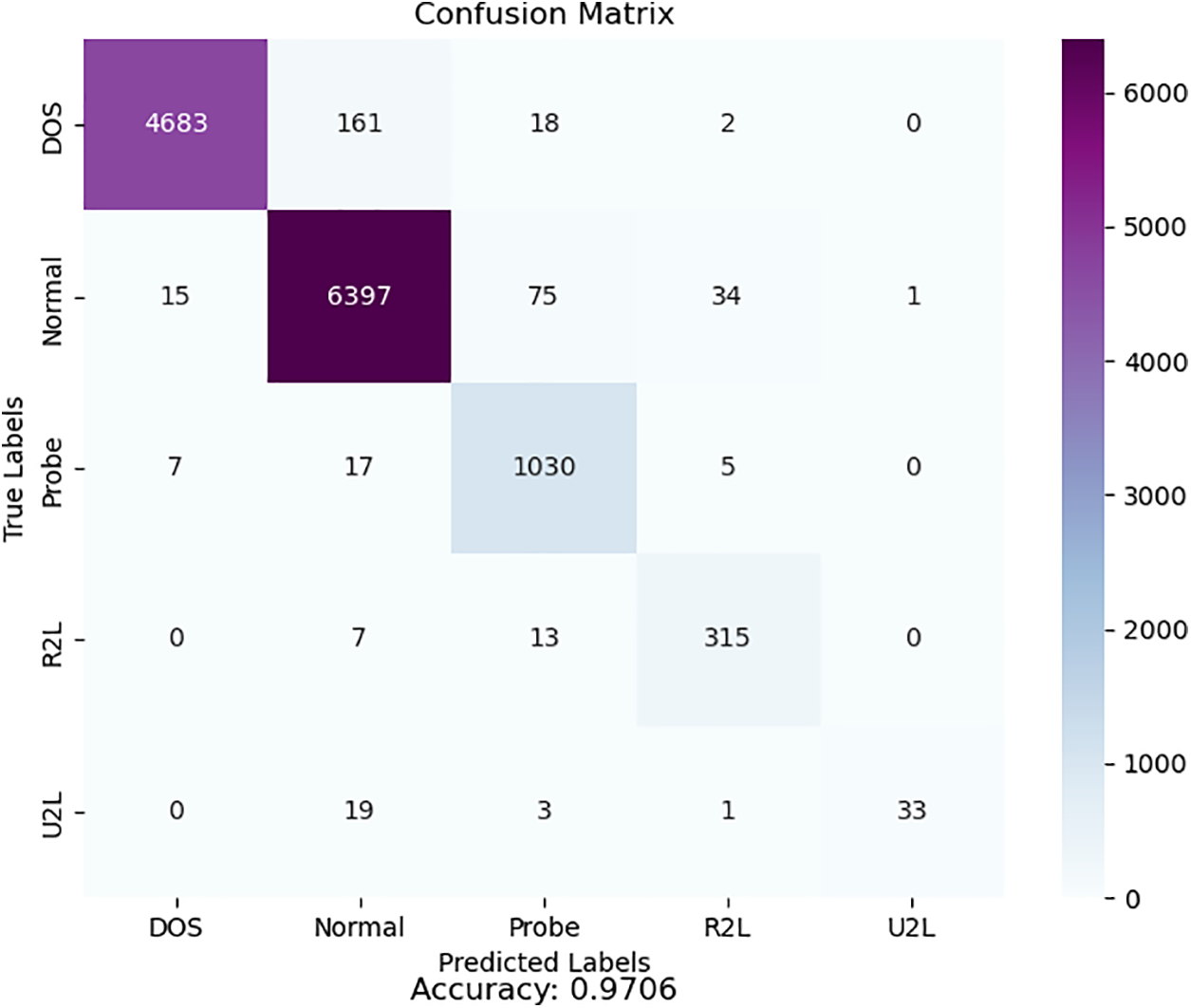
Figure 4: Confusion matrix diagram

The change in accuracy for each epoch during the training of the model is given in Fig. 5, it can be seen from this that the performance of the model is average in the early stages of training, but as the number of training rounds increases, the model performance steadily improves, and the model reaches its optimal state in the 36th training round.

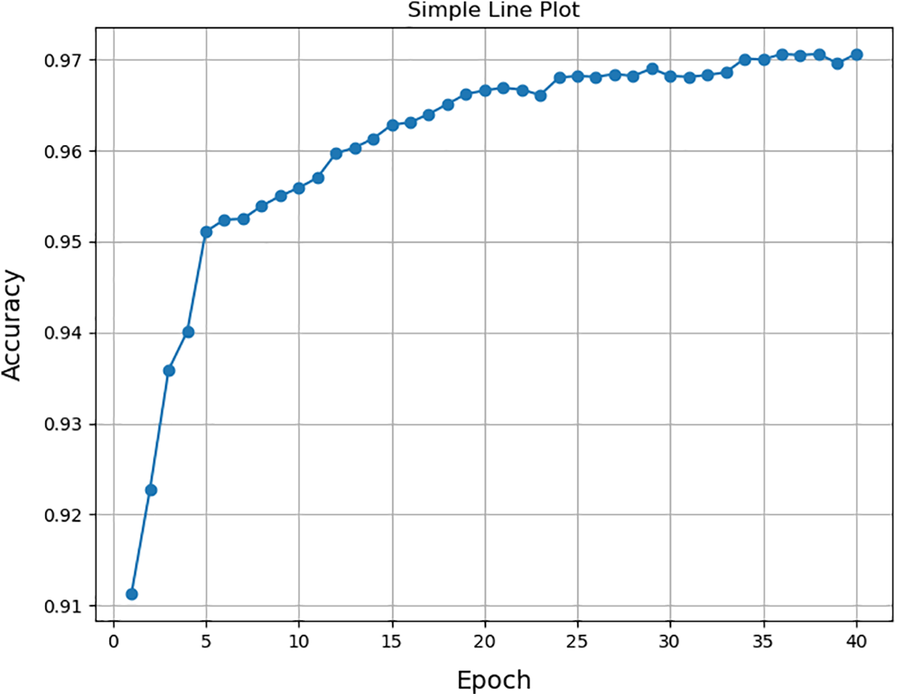
Figure 5: Model training line graph

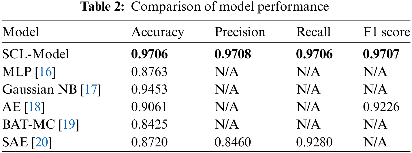
Table 2 displays performance comparisons between the SCL model and other models. When compared to other deep learning-based techniques already in use, these performance comparisons demonstrate how promising the experimental results of the SCL model are. Therefore, it is thought that one of the finest options for resolving the intrusion detection issue is our suggested approach.

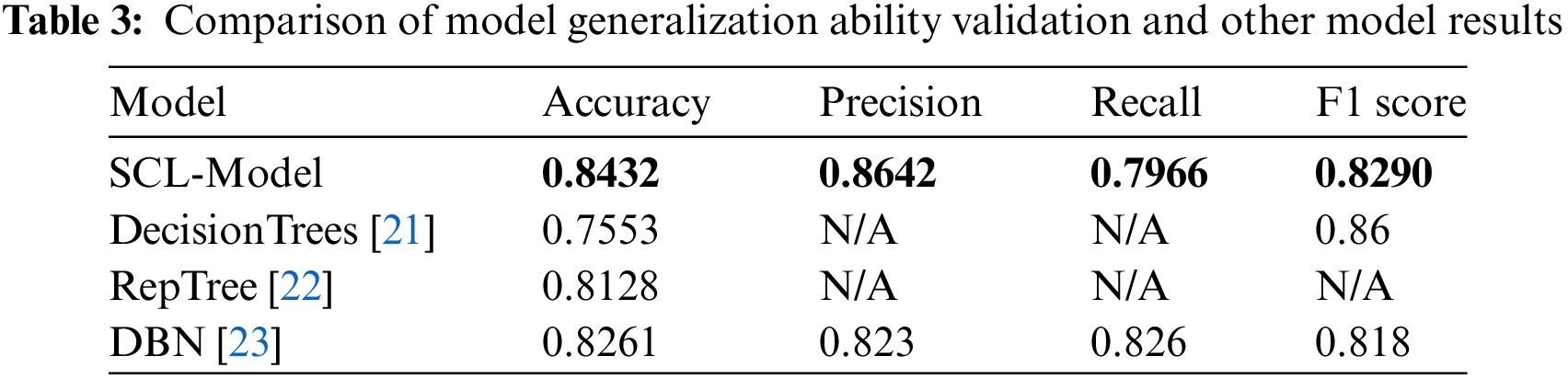
To verify the generalization performance of the model the UNSW-NB15 dataset is used to conduct experiments on the generalization ability of the model. The results of the multi-categorization experiments are shown in Table 3 in comparison with other models.

The optimal parameter settings for the model experiments in this paper are as follows: The model spiral convolution kernel is set to 64, the model learning rate is set to 0.001, the model batch size is set to 256, the first layer of LSTM is set to 64, and the second layer of LSTM is set to 128. In the ROC curve, the abscissa represents the false positive rate and the ordinate represents the true positive rate. In the figure, the larger the area surrounded by the curve and the closer the area is to 1, the better the performance of the model. The ROC plot is shown in Fig. 6.

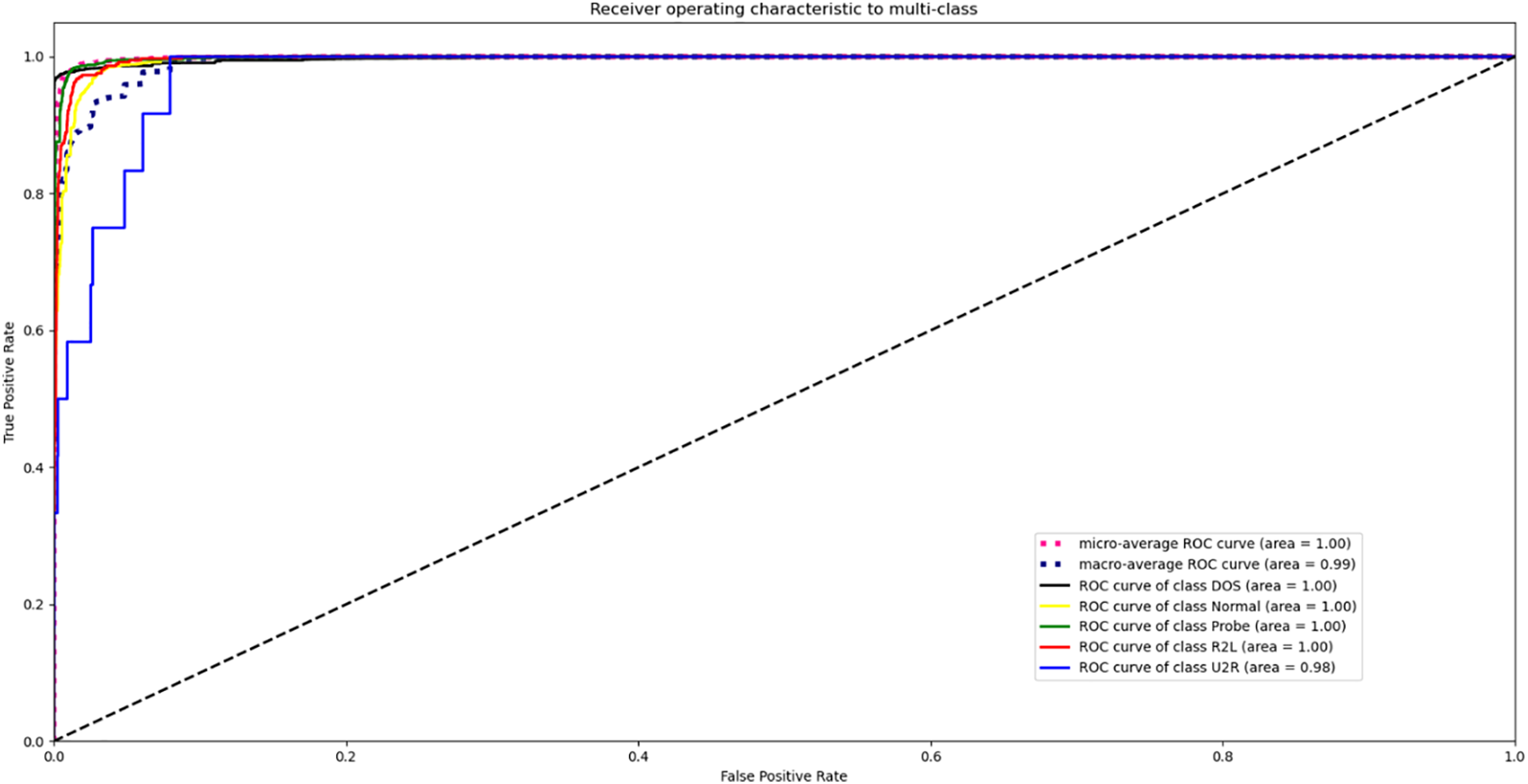
Figure 6: ROC plot of the optimal parameters of the model

Comparison of the training speed of the model in this paper with the training speed time of other deep learning models, using the time spent on a single round of epoch of the model in this paper as a unit time 1.0 as a benchmark comparison, as shown in Table 4.

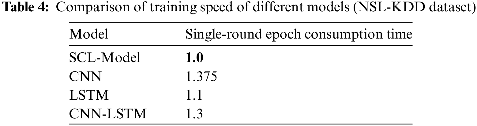
From the results, it can be seen that the model in this paper is greatly accelerated in training speed compared to the traditional CNN model, LSTM model, CNN-LSTM, and other models, and the memory occupation in training is also slightly decreased compared to other models.

3.2.2 Result Optimization

In today’s deep learning field attention mechanisms are widely used in all kinds of models and most of them have achieved good performance improvement. The attention mechanism is a technique that mimics the human attention mechanism in machine learning models. It allows the model to learn to combine different parts of the input data to produce more efficient results. The basic principle of the attention mechanism is to decompose the input data into multiple parts and then assign a weight to each part. These weights represent the importance of each section. These weights are then applied to the input data to generate a new input that contains all the important information.

To further improve the model performance, this paper introduces the multi-head attention [24] mechanism, and adds the multi-head attention mechanism between the spiral convolutional layer and the LSTM layer, to verify whether the attention mechanism can further optimize the model. The experimental results of multi-head attention with different numbers of heads are shown in Table 5.

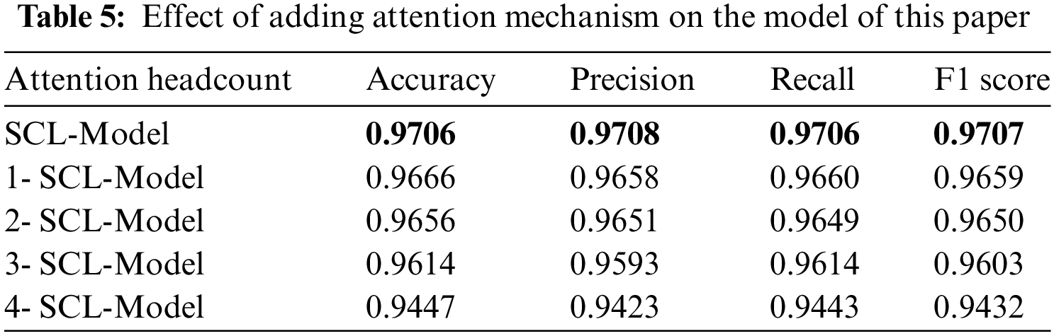
The performance of the experimental results is deplorable, the introduction of the attention mechanism did not optimize the model performance, and with the increase in the number of attention heads, the accuracy rate instead declined. And the single epoch training time of the model is significantly longer.

For this phenomenon, this paper believes that the reason is that the attention head in the neural network is actually a matrix form, which is a linear transformation of the input data, and the result obtained after the transformation is discrete rather than continuous, which may not be able to truly express the real target probability distribution. There are errors with the real target, and the more attention heads, the greater the accumulated errors in the calculation process, and ultimately lead to poor model performance.

However, the introduction of attention mechanism is still exploratory for deep learning intrusion detection models, there are very many kinds of attention mechanisms, such as Sparse Attention [25], CBAM Attention [26], FlashAttention [27], Coordinate Attention [28], etc., and all of these attention mechanisms have achieved good results in different model domains, and it remains one of the best ways to optimize the model in today’s deep learning domain.

4  Conclusion

In this paper, for the current intrusion detection model accuracy is not high, the training convergence time is long, the model training occupies a large amount of memory, and other issues, this paper proposes the integration of spiral convolution deep learning intrusion detection model-SCL model, the experimental results show that the model in this paper compared to the previous model has a fast convergence speed, the model training occupies a small amount of memory, the accuracy is high, and it has a good classification and detection performance. However, SCL-model still has its limitations. It has not been able to obtain excellent performance for high-dimensional data sets, and it has not been able to accurately detect a few class samples for data sets. In the future, consider using more complex network structures and data enhancement methods to solve these two types of problems.

Acknowledgement: The authors would like to thank the editors and reviewers for their valuable work, as well as the supervisor for their valuable support during the research process.

Funding Statement: The current work was supported by the Gansu University of Political Science and Law Key Research Funding Project in 2018 (GZF2018XZDLW20) and Gansu Provincial Science and Technology Plan Project (Technology Innovation Guidance Plan) (20CX9ZA072).

Author Contributions: Study conception and design: Fei Wang, Zhen Dong; data collection: Zhen Dong; analysis and interpretation of results: Fei Wang, Zhen Dong; draft manuscript preparation: Zhen Dong. All authors reviewed the results and approved the final version of the manuscript.

Availability of Data and Materials: The data that support the findings of this study are available on request from the corresponding author, Z D, upon reasonable request.

Conflicts of Interest: The authors declare that they have no conflicts of interest to report regarding the present study.

References

1. J. I. A. Fan and L. Z. Kong, “Intrusion detection algorithm based on convolutional neural network,” Trans. Beijing Inst. Technol., vol. 37, no. 12, pp. 1271–1275, 2017. doi: 10.15918/j.tbit1001-0645.2017.12.011. [Google Scholar] [CrossRef]

2. Y. Chang, W. Li, and Z. Yang, “Network intrusion detection based on random forest and support vector machine,” in 2017 IEEE Int. Conf. Comput. Sci. Eng. (CSE) and IEEE Int. Conf. Embed. Ubiquitous Comput. (EUC), Guangzhou, China, 2017, pp. 635–638. doi: 10.1109/CSE-EUC.2017.118. [Google Scholar] [CrossRef]

3. J. Jiang, X. Jing, B. Lv, and M. Li, “A novel multi-classification intrusion detection model based on relevance vector machine,” in 2015 11th Int. Conf. Comput. Intell. Secur. (CIS), Shenzhen, China, 2015, pp. 303–307. doi: 10.1109/CIS.2015.81. [Google Scholar] [CrossRef]

4. A. Yulianto, S. Parman, and A. S. Novian, “Improving adaboost-based intrusion detection system (IDS) performance on CIC IDS, 2017 dataset,” J. Phys.: Conf. Ser., vol. 1192, pp. 2–14, 2019. doi: 10.1088/1742-6596/1192/1/012018. [Google Scholar] [CrossRef]

5. C. Yin, Y. Zhu, J. Fei, and X. He, “A deep learning approach for intrusion detection using recurrent neural networks,” IEEE Access, vol. 5, pp. 21954–21961, 2017. doi: 10.1109/ACCESS.2017.2762418. [Google Scholar] [CrossRef]

6. S. C. Wang and S. P. Chen, “An improved model of anomalous traffic intrusion detection based on the residual network,” in Small Microcomput. Syst., 2021. doi: 10.20009/j.cnki.21-1106/TP.2022-0287. [Google Scholar] [CrossRef]

7. R. Panigrahi et al., “A consolidated decision tree-based intrusion detection system for binary and multiclass imbalanced datasets,” Mathematics, vol. 9, no. 7, pp. 751, 2020. doi: 10.3390/math9070751. [Google Scholar] [CrossRef]

8. S. M. Kasongo and Y. Sun, “Performance analysis of intrusion detection systems using a feature selection method on the UNSW-NB15 dataset,” J. Big Data, vol. 7, no. 1, pp. 1–20, 2020. doi: 10.1186/s40537-020-00379-6. [Google Scholar] [CrossRef]

9. R. Takahashi, T. Matsubara, and K. Uehara, “Data augmentation using random image cropping and patching for deep CNNs,” IEEE Trans. Circuits Syst. Video Technol., vol. 30, no. 9, pp. 2917–2931, 2019. doi: 10.1109/TCSVT.2019.2935128. [Google Scholar] [CrossRef]

10. M. Abdel-Nasser and K. Mahmoud, “Accurate photovoltaic power forecasting models using deep LSTM-RNN,” Neural Comput. & Appl., vol. 31, no. 7, pp. 2727–2740, 2019. doi: 10.1007/s00521-017-3225-z. [Google Scholar] [CrossRef]

11. G. Bouritsas, S. Bokhnyak, S. Ploumpis, M. Bronstein, and S. Zafeiriou, “Neural 3D morphable models: Spiral convolutional networks for 3D shape representation learning and generation,” in Proc. IEEE/CVF Int. Conf. Comput. Vis., Seoul, Korea, Oct. 27–Nov. 02, 2019, pp. 7213–7222. [Google Scholar]

12. J. Dai et al., “Deformable convolutional networks,” in 2017 IEEE Int. Conf. Comput. Vis. (ICCV), Venice, Italy, Oct. 22–29, 2017, pp. 764–773. [Google Scholar]

13. C. Chen, K. Li, S. G. Teo, X. Zou, K. Li and Z. Zeng, “Citywide traffic flow prediction based on multiple gated spatio-temporal convolutional neural networks,” ACM Trans. Knowl. Discov. Data, vol. 14, no. 4, pp. 1–23, 2020. doi: 10.1145/3385414. [Google Scholar] [CrossRef]

14. M. Tavallaee, E. Bagheri, W. Lu, and A. A. Ghorbani, “A detailed analysis of the KDD CUP 99 data set,” in 2009 IEEE Symp. Comput. Intell. Secur. Defense Appl., Ottawa, Canada, Jul. 8–10, 2009. doi: 10.1109/CISDA.2009.5356528. [Google Scholar] [CrossRef]

15. N. Moustafa and J. Slay, “UNSW-NB15: A comprehensive data set for network intrusion detection systems (UNSW-NB15 network data set),” in 2015 Military Commun. Inform. Syst. Conf. (MilCIS), Canberra, Australia, Nov. 10–12, 2015. [Google Scholar]

16. A. Sarkar, H. S. Sharma, and M. M. Singh, “A supervised machine learning-based solution for efficient network intrusion detection using ensemble learning based on hyperparameter optimization,” Int. J. Inf. Tecnol., vol. 15, no. 1, pp. 423–434, 2023. doi: 10.1007/s41870-022-01115-4. [Google Scholar] [CrossRef]

17. K. Bong and J. Kim, “Analysis of intrusion detection performance by smoothing factor of Gaussian NB model using modified NSL-KDD dataset,” in 2022 13th Int. Conf. Inform. Commun. Technol. Converg. (ICTC), Jeju Island, Korea, Oct. 19–21, 2022. [Google Scholar]

18. W. Xu, J. Jang-Jaccard, A. Singh, Y. Wei, and F. Sabrina, “Improving performance of autoencoder-based network anomaly detection on NSL-KDD dataset,” IEEE Access, vol. 9, pp. 140136–140146, 2021. doi: 10.1109/ACCESS.2021.3116612. [Google Scholar] [CrossRef]

19. T. Su, H. Sun, J. Zhu, S. Wang, and Y. Li, “BAT: Deep learning methods on network intrusion detection using NSL-KDD dataset,” IEEE Access, vol. 8, pp. 29575–29585, 2020. doi: 10.1109/ACCESS.2020.2972627. [Google Scholar] [CrossRef]

20. S. Gurung, M. K. Ghose, and A. Subedi, “Deep learning approach on network intrusion detection system using NSL-KDD dataset,” Int. J. Comput. Netw. Inf. Secur., vol. 11, no. 3, pp. 8–14, 2019. doi: 10.5815/ijcnis.2019.03.02. [Google Scholar] [CrossRef]

21. S. Meftah, T. Rachidi, and N. Assem, “Network based intrusion detection using the UNSW-NB15 dataset,” Int. J. Comput. Digit. Syst., vol. 8, no. 5, pp. 478–487, 2019. doi: 10.12785/ijcds/080505. [Google Scholar] [CrossRef]

22. M. BBelouch, S. El Hadaj, and M. Idhammad, “A two-stage classifier approach using reptree algorithm for network intrusion detection,” Int. J. Adv. Comput. Sci. Appl., vol. 8, no. 6, pp. 1–12, 2017. doi: 10.14569/issn.2156-5570. [Google Scholar] [CrossRef]

23. R. Shrestha, “A mapreduce-based deep belief network for intrusion detection,” Doctoral dissertation, Pulchowk Campus, 2017. [Google Scholar]

24. H. Zheng, J. Fu, T. Mei, and J. Luo, “Learning multi-attention convolutional neural network for fine-grained image recognition,” in Proc. IEEE Int. Conf. Comput. Vis., Venice, Italy, Oct. 22–29, 2017. [Google Scholar]

25. Y. Tay, D. Bahri, L. Yang, D. Metzler, and D. C. Juan, “Sparse sinkhorn attention,” in Int. Conf. Mach. Learn., Vienna, Austria, Jul. 12–18, 2020. [Google Scholar]

26. S. Woo, J. Park, J. Y. Lee, and I. S. Kweon, “CBAM: Convolutional block attention module,” in Proc. Eur. Conf. Comput. Vis. (ECCV), Munich, Germany, Sep. 8–14, 2018. [Google Scholar]

27. T. Dao, D. Fu, S. Ermon, A. Rudra, and C. Ré, “Flashattention: Fast and memory-efficient exact attention with io-awareness,” Adv. Neural Inf. Process. Syst., vol. 35, pp. 16344–16364, 2022. [Google Scholar]

28. Q. Hou, D. Zhou, and J. Feng, “Coordinate attention for efficient mobile network design,” in Proc. IEEE/CVF Conf. Comput. Vis. Pattern Recognit., Nashville, TN, USA, Jun. 20–25, 2021. [Google Scholar]