An Intelligent Framework for Resilience Recovery of FANETs with Spatio-Temporal Aggregation and Multi-Head Attention Mechanism

1  Introduction

With its high mobility, low cost, and strong flexibility, unmanned aerial vehicle (UAV) swarm has been widely used in various applications, such as surveillance [1], agriculture [2], rescue [3], etc. In these applications, large numbers of UAVs cooperate with others as a UAV swarm relying on communicating with one another, thus the connectivity of the communication network is a vital necessity for a UAV swarm. However, the harsh working environment and complicated mission requirements make it difficult to ensure the connectivity of the networks. As a kind of flying Ad hoc network (FANET), the occurrence of communication links between UAVs depends on the communication radius and location distribution [4]. Although expanding the communication radius of each drone seems intuitive and effective, however, it is not practical due to the energy constraint and the fading effect [5]. At the same time, a certain amount of redundant drones can not ensure resilient connectivity when more drones are damaged. Thus, changing location deployment has become a common strategy to keep the network resilient after destruction.

However, there are still some challenges to quickly rebuilding network connectivity by redeploying locations. First, when drones are destroyed, it is difficult to model the network structure consisting of changing nodes and edges under continuous destruction [6]. The second challenge is how to further reduce self-recovery time with real-time communication and storage limits, which is closely related to network resilience. At last, quick network connectivity recovery and adequate coverage have contradicting focuses. It is seemingly straightforward to rebuild the connectivity by drones moving closer to each other. However, to ensure the network coverage performance each drone should cover enough non-overlapping area to avoid duplicate effort. Thus, how to balance the network coverage and network connectivity needs to be carefully considered.

To tackle the challenges above, we propose a graph attention network (GAT)-based mechanism to recover both coverage and connectivity for a resilient swarm network against random destruction in this paper. The main contributions of our work are summarized as follows:

• We build a system recovery model for a swarm network from the perspective of engineering resilience. Our model considers both the coverage and the connectivity when serious damage happens.

• We propose a temporal aggregation graph generating method to provide a persistent connected graph structure for computing the combination of the drones’ location feature vectors. Our model is based on the historical and current location information of both destroyed drones and remaining drones, which can still update the new location features on all nodes even if the node is isolated from other nodes in the current network.

• We incorporate structural information from the temporal aggregation graph into GAT. Simulation results show that the proposed methods can recover coverage and connectivity. At the same time, the results show that our methods reduce recovery time.

The remainder of the paper is organized as follows: Section 2 reviews the related work. Section 3 describes the system model, the temporal aggregation graph generating method, and the graph self-attention mechanism with the aggregation graph for feature vector updating. Section 4 presents simulation results and analysis of the proposed algorithm and Section 5 concludes the work.

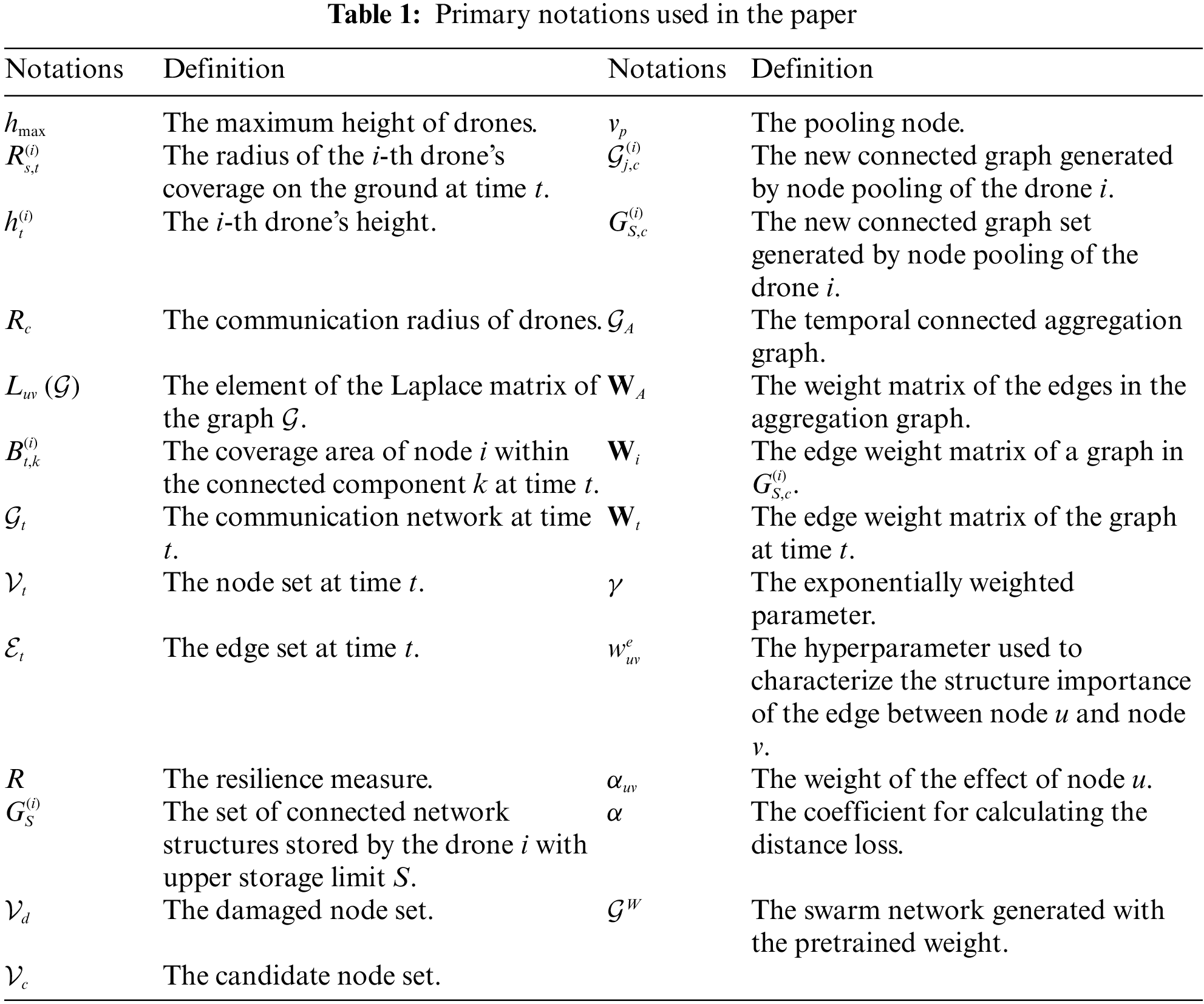
Most of the notations applied in this paper are standard. To ease readability, all the primary notations of the paper are listed in Table 1.

2  Related Works

Due to complicated mission requirements, the network is required to be self-adaptive to destructive events in the harsh working environment. The attribute measuring this dynamic process is usually called resilience. Resilience commonly measures the whole process of a system from interference, damage, and recovery. Currently, the resilience of swarm networks has received increasing attention [7–9]. However, the above methods only proposed metrics for evaluation but offered little specific guidance for keeping the swarm network resilient. Despite the lack of resilience-based mechanisms, some works are aiming at recovering the coverage and connectivity of swarm networks through deployment techniques.

Some studies proposed theoretical results of network coverage and connectivity by using geometric models to find analytical solutions under certain conditions [10]. For instance, Mozaffar et al. [11] utilized circle packing theory to determine the optimal three-dimensional location that maximizes the total coverage area of the swarm. Bai et al. [12] proposed an optimal deployment pattern that achieves full coverage and 2-connectivity when the communication radius equals the perception radius of each drone. However, the strict assumptions for these analytical models make it challenging to apply for the recovery of a highly dynamic swarm network [13].

Several studies attempted to recover the network based on iterative adjustment of drones’ locations. For instance, Sharma et al. [14] introduced a scheme to recover coverage and connectivity by recursively relocating mobile nodes and enabling backup nodes. Chen et al. [15] proposed a potential field-based network approach depending upon perceiving network damage, which can recover the network connectivity in flight paths. Qi et al. [16] presented a network topology construction method based on connected dominating sets, which iteratively adjusts transmission power and position to achieve desired fault tolerance levels. However, due to multiple iterations, these works involve extensive communication and redirection during the recovery, which potentially hinders rapid recovery after massive destruction events happen.

Several studies have employed machine learning algorithms, such as graph neural networks (GNN) [17,18], deep learning techniques, and other approaches [19,20], to address the problem. For instance, Mou et al. [18] proposed a graph convolutional neural network (GCN)-based algorithm for UAV trajectory planning to rebuild the communication connectivity of the network. However, this approach relies on a lot of storage space for meta parameters to adapt to changes in the number of network nodes. Zhang et al. [20] introduced a reinforcement learning method based on an artificial potential field for a robust network design. Nevertheless, machine learning algorithms demand massive computational resources and may have poor scalability across different system models.

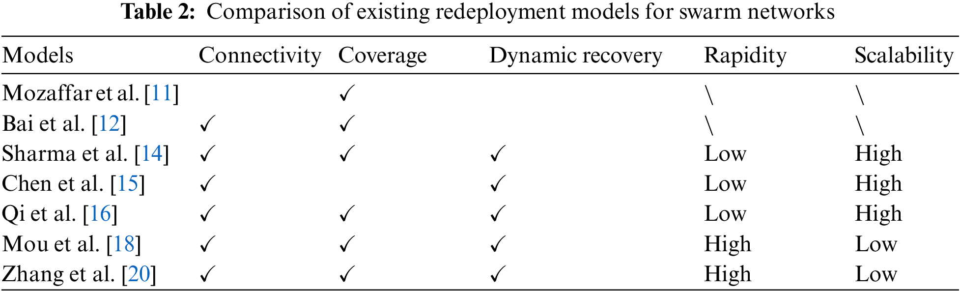
As shown in Table 2, the existing models through deployment techniques cannot meet all the requirements of resilient recovery.

3  Proposed Framework

3.1 The Resilience Optimization Model

We consider a square geographical area with a diameter of L, as shown in Fig. 1, where N UAVs are deployed as a swarm to fulfill the mission in this area. In this model, we assume that the drones are homogeneous, i.e., each drone has the same transmit power and field angle. To model the coverage and connectivity of a network, we provide the following definition.

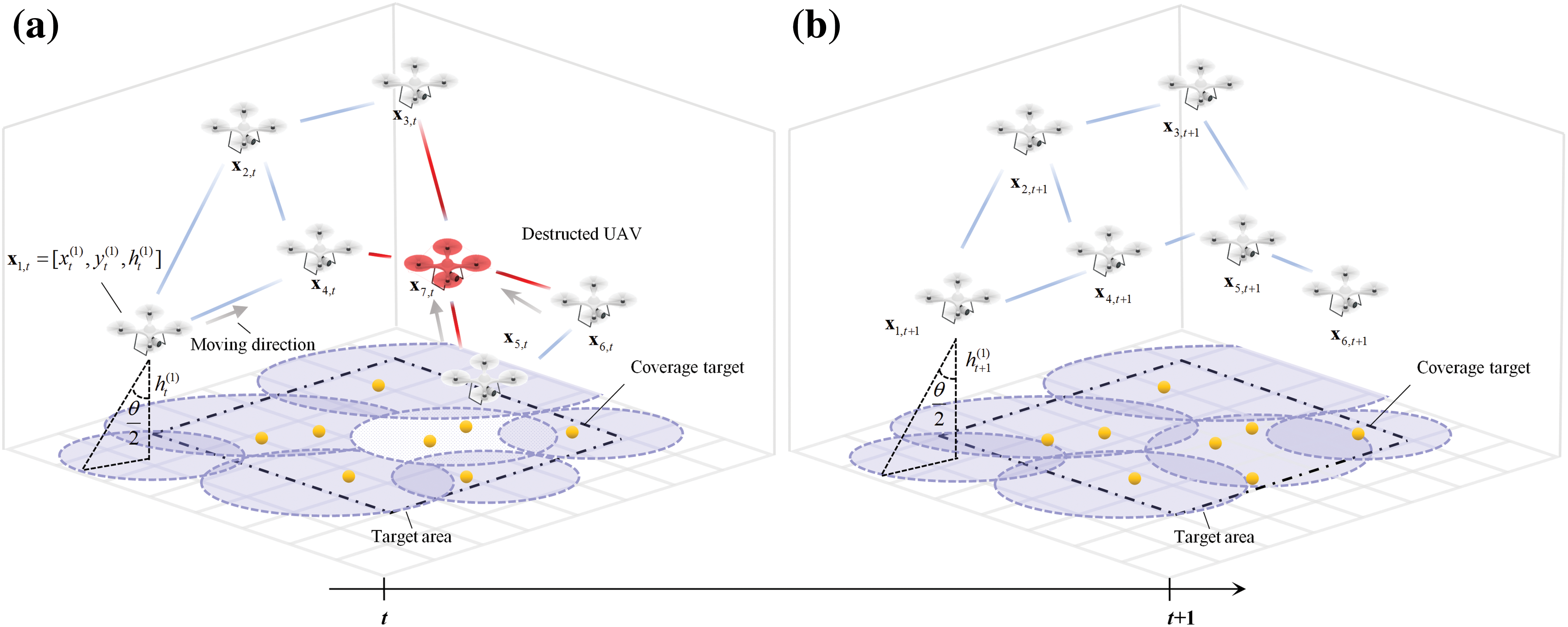
Figure 1: The recovery process for the coverage and connectivity of a FANET by redeploying locations. (a) The network is being destroyed. We assume the initial deployment forms a connected communication network. Destruct a UAV randomly at time t and thus destroy the connected network. Then the remaining UAVs react against the destruction and try to restore the by redeploying their locations. (b) The network after recovery by redeploying locations

Definition 1 (Covering and Connected Network): A covering and connected network denotes a network composed of N UAVs located in a three-dimensional location set, which can cover the entire geographical area while ensuring network connectivity.

The above definition has generality since it can describe various air-to-ground coverage missions, including wireless communication, monitoring, lighting, or other services for ground targets. As shown in Fig. 1, Although the coverage radius will increase with the height of a UAV, increasing the height will also lead to further distance between the UAV and the target, which may lower the service level of certain missions. Thus, we assume the service level threshold is ε, the maximum height hmax can be defined as

hmax=max{h|Ξ(h,ζ,θ)≥ε},(1)

where Ξ can be any well-defined service level measure, ζ can be initial energy or information provided by the drone for the mission, θ is the drone’s coverage field angle to the ground. Then, the radius of the i-th drone’s coverage on the ground at time t can be calculated by

Rs,t(i)=ht(i)tan⁡θ2,ht(i)≤hmax,(2)

where ht(i)is the i-th drone’s height to the ground at time t. Here, we consider the network to be homogeneous, thus all drones share the same field angle θ and the maximum height hmax.

In this paper, the FANET between UAVs at time t is modeled as a communication network 𝒢t={𝒱t,ℰt} consisting of a node set 𝒱t and an edge set ℰt, with the position features {xv,t∈R3,∀v∈𝒱t} of the drone v. Considering the air-to-air communication links with no ground obstacle, we assume the signal power threshold that can be received is P0, the communication radius Rc can be calculated as

Rc=max{r|10ηlog10⁡(4πrfcc)+pξ(r)≤P+G1+G2−P0},(3)

where r is the distance between drones, fc is the carrier frequency, η>0 is the path loss exponent, pξ(r) is the small-scale fading effect, G1 and G2 are the constant antenna gains of the receiving and transmitting and P is the drone’s transmit power.

According to the fading effect, communication links only exist between nodes within a certain distance. Specifically, the communication range is defined as Rc, the necessary and sufficient condition for an edge euv,t∈ℰt is the distance d(u,v)≤Rc between two nodes in three-dimensional space [21]. For a FANET, the definition of a connected network is as follows.

Definition 2 (Connected Network): In a coverage area, if any two drones in the FANET can always transmit information to each other through the routing, that is, given a network 𝒢t, if any two nodes can find a path between them, it is said that the network 𝒢t is connected.

Based on spectral graph theory, in a network with only one component, there is only one eigenvector with eigenvalue zero, the vector 1 (or multiples of it). All other eigenvectors must have non-zero eigenvalues. Thus, to check whether the network is connected, we calculate the eigenvalues of the Laplace matrix of the network. Define the adjacency matrix of network 𝒢 as A(𝒢), each element Luv(𝒢) of the Laplace matrix L(𝒢) of the graph can be calculated as follows:

Luv(𝒢)=δuv∑vAuv(𝒢)−Auv(𝒢),(4)

where δuv is Kronecker delta function, when u=v, δuv=1, otherwise δuv=0. It is known that for an undirected graph 𝒢 with non-negative edge weight, the algebraic multiplicity m0 of the zero eigenvalues of the Laplace matrix L(𝒢) is equal to the number of connected components C(𝒢) of the network. In graph theory, the connected component (or only the component) of an undirected graph is defined as a subgraph in which any two vertices are connected through any path. Thus when m0=C(𝒢)=1, there is only one connected component in a connected graph, i.e., the network is connected [22].

When serious destruction happens, the connected network may be divided into a set of connected components. However, the neighbors of the destroyed drones can sense the destruction and update their neighbor sets. Then the drones in the same connected network share real-time location information and the existing situation of all drones in the network. Based on the location information, the remaining drones attempted to recover the network by adjusting their location.

The goal of our work is to provide a mechanism for keeping the network covering and connected resiliently. Denote the coverage area of node i within the connected component k as Bt,k(i)⊂RL×L can be written as a set of point x as follows:

Bt,k(i)={x|d(i,x)≤Rs,t(i)}.(5)

Then the network performance of coverage and connectivity can be defined as the average coverage of each connected component as follows:

B(𝒢t)=1M∑k=1M|∪i=1|𝒱tk|Bt,k(i)|/L2,(6)

where M is the number of connected components and |𝒱tk| is the number of nodes within the k-th connected component. Here, for each connected component, we consider the ratio of the total non-repeated coverage area of all nodes to the target area as the coverage performance. Denote the acceptable performance level as 1, then when a failure occurs, resilience can be measured as [23]

R=∫t0t0+T∗Q(t)T∗,(7)

Rmin=(T∗−ΔBT)/T∗=1−ΔBT/T∗,(8)

where Q(t) is the performance measure, ΔB is the percentage of the maximum performance loss after destruction, T is the time required for full recovery, and T∗ is the time interval to determine performance loss.

As shown in Fig. 2, when Q(t)≥(1−ΔB), R≥Rmin=1−ΔBT/T∗. If we always aim to fully recover the performance to the acceptable level, the performance loss ΔB and the time length T∗ are both constants after a certain destruction happens. With the fixed ΔB and T∗, the resilience only depends on recovery time T. Thus, maximizing resilience is equivalent to minimizing the recovery time T. Then, the resilience goal of the recovery problem for a covering and connected network can be formulated as

P1:max{x^1,x^2,⋯,x^n}minR=max{x^1,x^2,⋯,x^n}1−ΔBT/2T∗=min{x^1,x^2,⋯,x^n}T,(9)

T≤maxi∈𝒱t‖x^i,t−xi,t‖2,(10)

when the flying velocity vf is fixed, and the recovery time T of the swarm is determined by the maximum displacement in the deployment plan. Thus we can formalize the problem as follows:

P1:min{x^1,x^2,⋯,x^n}maxi∈𝒱t‖x^i,t−xi,t‖2,s.t.B(𝒢^t)=1,C(𝒢^t)=1,hi,t≤hmax,Q(t)≥(1−ΔB).(11)

where {x^1,x^2,⋯,x^n} is the planned location set and 𝒢^t is the formed network with the planned location under communication range Rc.

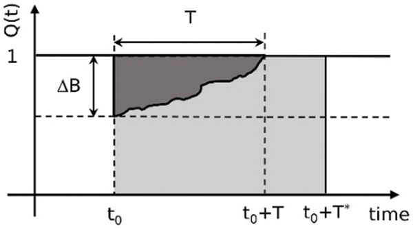
Figure 2: An interpretation of the resilience loss

In the next parts, we will describe the specific procedures of the optimization algorithm. The objective is to maximize the resilience measure defined in formula (11). We describe the two primary parts of our algorithm: Spatial-temporal connected graph generation and the multi-head graph neural network. The whole framework of the algorithm is summarized in Fig. 3.

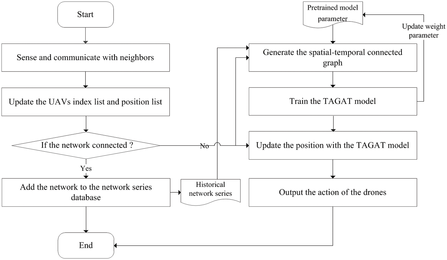
Figure 3: The research flow diagram of proposed framework

3.2 Spatial-Temporal Connected Graph Generation

Noticing that the graph neural network is good at representing graph data features, we developed an idea using a graph neural network to learn the mapping from the initial locations of drones to optimized locations. However, if the network 𝒢t at time step t has isolated nodes or connected components, it is difficult to update the position features of the isolated nodes on the graph neural network structure according to it. To ensure the features can be updated on all the nodes, we propose a connected graph generation method.

We denote the set of connected network structures during running stored by the drone i as GS(i)={𝒢1(i),𝒢2(i),⋯,𝒢S(i)}, where S is the storage limit. With the upper limit, only the latest connected graph series will be retained by updating the sequence as a queue. When the network 𝒢t of the swarm is not connected, we try to aggregate the connected networks in GS(i) and the network 𝒢t to generate a connected graph as the basis for the GNN model.

Due to the decrease in the number of nodes after each disruption, the number of connected graph nodes at different time steps in GS(i) varies. Meanwhile, the node set of any connected network contains the destroyed nodes, which should not be aggregated to the network 𝒢t after the destruction [24]. To address this issue, we propose a node pooling method that removes damaged nodes from GS(i)={𝒢1(i),𝒢2(i),⋯,𝒢S(i)} while preserving edge connectivity within the remaining node set.

The steps of this method are as follows: As shown in Fig. 4, we perform the pooling operation on the graph in the set GS(i) sequentially.

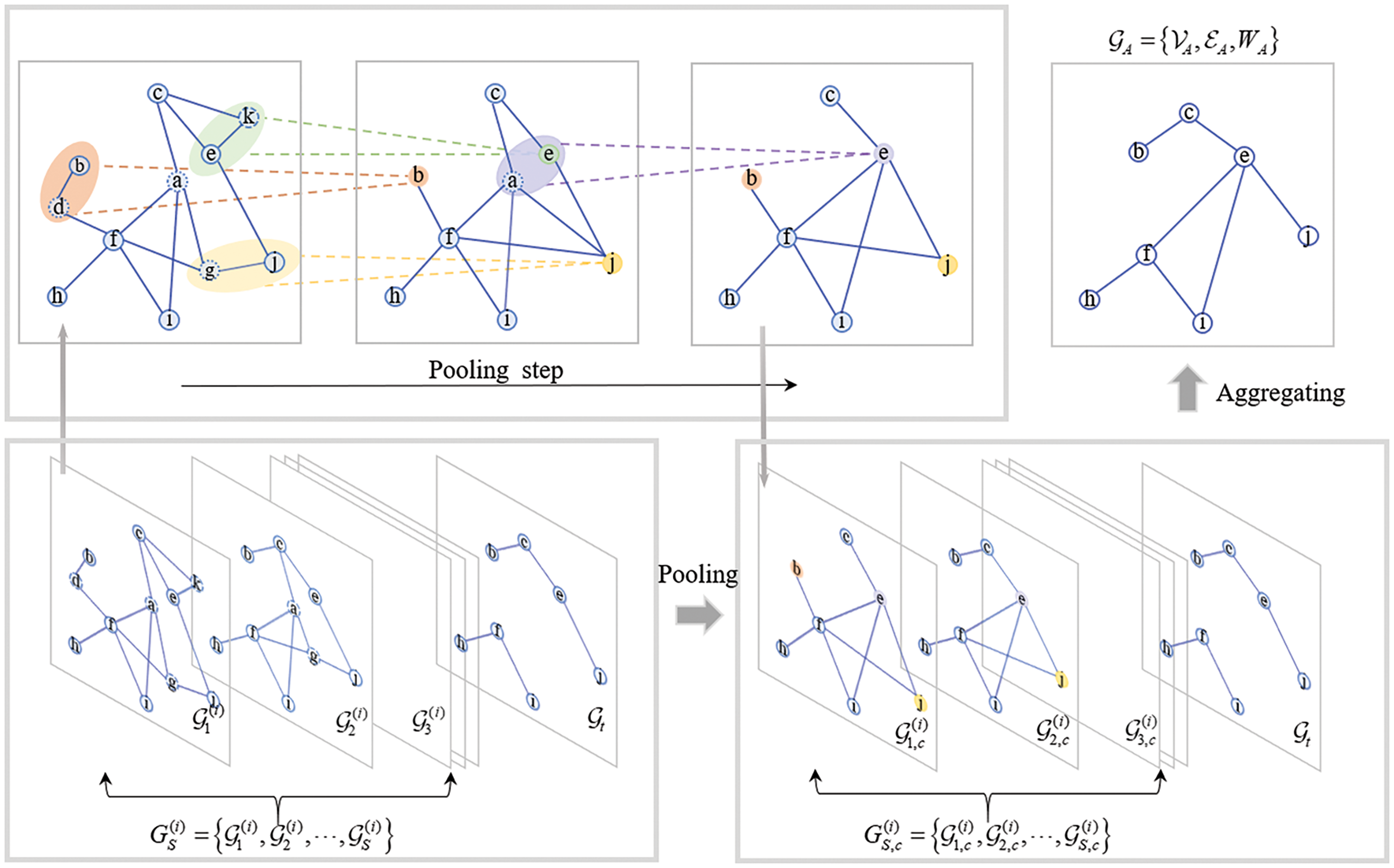
Figure 4: The generation process of temporal aggregation connected network. For example, the node set 𝒱t of the network at time t equals the node set 𝒱A of the network after aggregation, i.e., 𝒱A=𝒱t. Node pooling is performed on each graph in the graph set GS(i). For an instance of 𝒢1(i)∈GS(i), where the pooling nodes are b, e, and j, we merge the connections on d, a, k, and g with the corresponding pooling nodes to form a new connected graph 𝒢1,c(i). Finally, we aggregate the graphs in GS(i) into an aggregate graph 𝒢A according to formula (1)

Specifically, for the j-th graph 𝒢j(i)={𝒱j(i),ℰj(i)}, select node v from the damaged node set 𝒱d={v|v∈𝒱j(i),v∉𝒱t} in sequence and search for the pooling node of the damaged node v in the candidate node set 𝒱c={v|v∈(𝒱j(i)−𝒱d)}. The selection rule is to select the node in 𝒱c with the smallest distance to node v as the pooling node vp. Specifically, the pooling node vp can be determined as

vp=arg⁡minΔ(vc,v),vc∈𝒱c,(12)

where Δ(⋅) can be any well-defined distance measure, we use the Euclidean distance in this paper. Then, the edges on the destroyed node v are retained on the pooling node to generate a new edge set ℰj,c(i), i.e., the pooling node plays the same role as the destroyed node for the network. Finally, delete the nodes in the damaged node set 𝒱d from the node set 𝒱j(i)to generate a new point set 𝒱j,c(i), and delete the corresponding edge {euv|euv∈ℰj,c(i),∀u,v∈𝒱d} on the damaged node from the edge set ℰj,c(i) to obtain a new graph 𝒢j,c(i)={𝒱j,c(i),ℰj,c(i)}, which can be written as

𝒢j,c(i)={𝒱j,c(i),ℰj,c(i)},𝒱j,c(i)=𝒱j(i)−𝒱d(i),ℰj,c(i)=ℰj(i)−{euv|euv∈ℰj,c(i),∀u∈𝒱d}.(13)

By preserving all edges on remaining nodes during deletion, connectivity within newly formed graphs is ensured. Denote the new connected graph set generated by node pooling as GS,c(i)={𝒢1,c(i),𝒢2,c(i),⋯,𝒢S,c(i)}. Then combines the graphs in GS,c(i) with the network 𝒢t to form a temporal connected aggregation graph 𝒢A={𝒱A,ℰA,WA}, which can be written as

𝒢A={𝒱A,ℰA,WA},𝒱A=𝒱t,ℰA=⋃i=1Sℰj,c(i),WA(i,j)={1,eij∈ℰA0,eij∉ℰA.(14)

We assume the impact of a historical graph in GS,c(i)={𝒢1,c(i),𝒢2,c(i),⋯,𝒢S,c(i)} diminishes over time. Hence, exponentially weighted average [25] is employed to process the graph time series. Denote the weight matrix of the edges in the aggregation graph 𝒢A as WA and assume the weights of all edges of any historical graph and 𝒢t are both 1, then

WA=γWS+γ(1−γ)WS−1+⋯+γS−1(1−γ)W1+(1−γ)Wt,(15)

where Wi,i∈{1,2,⋯,S} denotes the edge weight matrix of a graph in GS,c(i), Wt denotes the edge weight matrix of 𝒢t, γ denotes the exponentially weighted parameter. The spatial-temporal connected graph generation can be described below.

Step 1: We calculate the Euclidean distance from the destroyed node to other nodes in the network, then update the nearest node. We record and determine central nodes for the spatial aggregation based on the minimum Euclidean distance between nodes.

Step 2: We transfer the edges on the damaged node to the corresponding aggregation node. It should be noted that when operating on the whole adjacency matrix to avoid the potential interference of operations on the subsequent nodes. Finally, delete the edges on the damaged nodes as a whole.

Step 3: For each spatial-temporal network, we repeat steps 1 to 2 and record the connected network structure formed for each spatial-temporal network until there is no spatial-temporal network in the temporal graph set.

Step 4: We aggregate the connected spatial-temporal network according to the formula (15).

Based on the above mechanism, we can generate a spatial-temporal connected graph according to Algorithm 1.

3.3 The Multi-Head Graph Network with Structure Importance Hyperparameter for Target Location Generation

To generate the target location for the recovery of the swarm, We propose the temporal aggregation graph attention network (TAGAT) to map the location after destruction to the new location for quick recovery. GCN or Graphsage was employed by some existing methods [26]. However, both GCN and Graphsage are based on the assumption that the effect of each dimension of each neighboring node’s features on the central node features is homogeneous, for instance, the effect of the distance in each direction on the Euclidean distance between nodes is the same in three-dimensional space for connectivity recovery. However, this assumption may not be suitable for coverage recovery. When considering coverage performance, the effect of height features and horizontal position features on the radius of ground horizontal projection is different, so it is necessary to consider using attention mechanisms to learn the difference between these features. The self-attention mechanism allows models to adaptively select key information based on task requirements when processing data, thereby focusing on important features and ignoring relatively unimportant ones. Therefore, using attention mechanisms can enhance the modeling ability of models for complex equipment system state changes. For example, Transformer models and their variants based on attention mechanisms have been widely used in fault diagnosis of mechanical systems [27,28]. Both Transformer and GAT utilize self-attention mechanisms to capture the correlation between inputs, while GAT is more suitable for graph-structured data. However, GAT lacks direct utilization of graph structure information of data, which makes GATs prone to underfitting in learning tasks related to structural features [29,30]. Thus, it is necessary to consider combining the temporal aggregation graph with GAT to improve the learning ability of the network.

We provide the definition of the graph attention operator. The input is graph data 𝒢={𝒱,ℰ,X}, where X∈R|𝒱|×D is the feature matrix of the nodes and D=3 is the dimensionality of the feature. Our goal is to output new feature vector representations Z∈R|𝒱|×3 of nodes.

The self-attention mechanism is calculated point by point, assuming the central node is v, the edge weights from neighboring node u to node v are calculated as follows:

euv=σ(wuve[Wxu‖Wxv])∀(u,v)∈ℰ,(16)

where W is a weight transformation applied to each node used to learn the weights between different features, wuve∈We is a hyperparameter used to characterize the structure importance of the edge between node u and node v, and the activation function σ selected is the LeakyReLU function. Here, the normalized Laplace matrix Lijrw is used to characterize the structural relationship between node v and neighboring node u [31], and the calculation formula is as follows:

We=−Lrw=D−1WA−IN,(17)

Lrw(i,j)={1 if i=j−WA(i,j)D(i,i) else .(18)

When i≠j, ∑k≠i|𝒱|wike=1, so the requirements of weight normalization are satisfied. Then the softmax function is used for nonlinear transformation, the weight of the effect of node u is

αuv=exp⁡(euv)∑k∈𝒩vexp⁡(ekv).(19)

Then, using a multi-head attention mechanism with K independent heads for calculating features, the new feature vector of the central node v can be obtained by averaging the weighted sum of the feature vectors of itself and neighboring nodes.

zv=1K∑k=1Kσ(∑u∈𝒩vαuv(k)W(k)xu),(20)

where the activation function σ is the LeakyReLU function. We use n-layer GAT layer stacking to increase learning ability as shown in Fig. 5, where the training parameter of the i-th layer is Wi={Wi(1),Wi(2),⋯,Wi(k)}. According to formula (8), the loss function with the weight of the multi-layer GAT network is calculated as

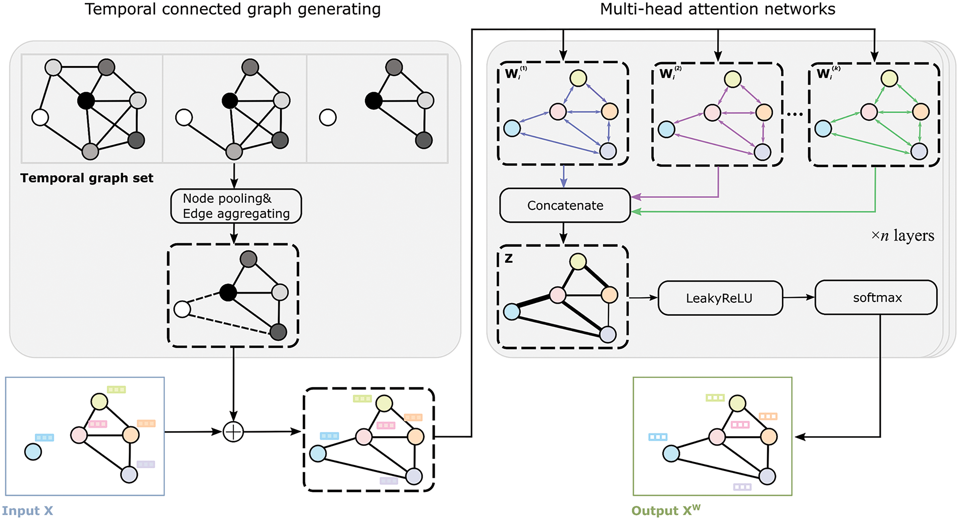
Figure 5: The structure of the temporal aggregation graph attention network. With the spatial-temporal connected graph as the backbones, TAGAT is composed of n multi-head attention layers. The k-th layer receives a topology matrix from the last layer and outputs a new topology matrix

Loss(W1,W2,⋯,Wn,X)=λB(1−B(𝒢W))⏟guarantee the coverage constraints+λC(C(𝒢W)−1)⏟guarantee the connectivity constraints+αmaxi∈𝒱t‖xiW−xi‖2⏟distance loss(21)

where λB and λC are the Lagrange multipliers are set as positive constants, xiW are the output matrix, and 𝒢W are the swarm network generated with the location xiW and the communication radius Rc. We define the coefficient α for calculating the distance loss as

α={1Br(𝒢W) if B(𝒢W)=11 else ,(22)

Br(𝒢W)=1M∑k=1M∑i=1|𝒱tk||Bt,k(i)|/L2,(23)

where M is the number of connected components, |𝒱tk| is the number of nodes within the k-th connected component. Here we calculate the total coverage area Br(𝒢W) as the performance redundancy level to characteristic the satisfaction of regional coverage requirements, which differs from the first term in (19) [32]. Through coefficient α, we tend to choose output locations with higher performance redundancy levels.

We use randomly generated pairs of the connected and non-connected graph to pretrain the network, then use pretraining parameters to accelerate the training speed of the algorithm in on-line execution as Fig. 6 shows. Specifically, a connected graph is randomly generated and a certain number of nodes are destroyed, if the generated graph is not connected, the damaged node number is recorded. The above connected graph and the non-connected graph are input into the network for training. Since the weights need to be retrained only when the number of network layers and dimension of features vary, and the weights Wi∈Rk×D can be applied to the networks with various numbers of nodes. Thus compared to GCN, TAGAT needs fewer parameters that need to be precalculated and stored.

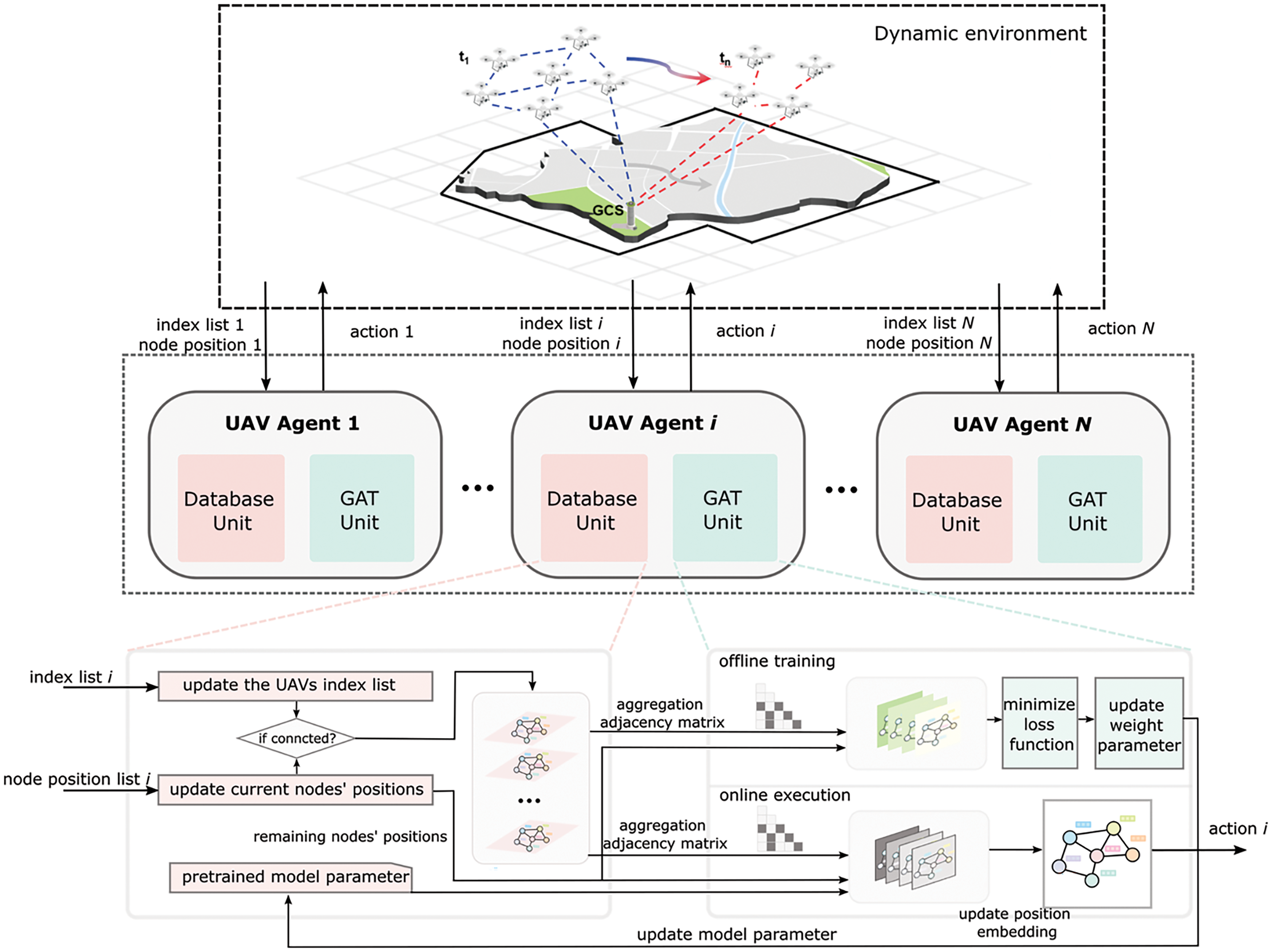
Figure 6: The structure of the temporal aggregation graph attention network. We highlight the interaction between the database unit and the GAT unit. The GAT consists of two parts: Offline training and online execution. With the pretrained parameter, the model can output the action efficiently. At the same time, the collected network data can be used in offline training, which updates the weight parameter to keep the model scalability with the few hyperparameters

4  Simulation Results

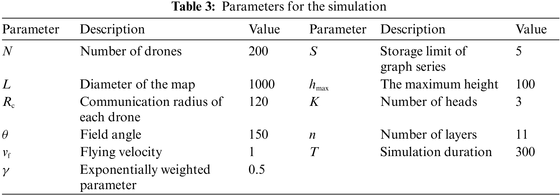
In the simulation, the initial swarm consists of 200 drones, with drones distributed in 1000 × 1000 × 100 patches space, thus the size of the target ground area to cover is 1000 × 1000 patches, as shown in Fig. 7. Due to the large number of drones, there is some redundancy in the network’s coverage of the ground area. However, under destruction, the coverage will be split with the components of the network. We apply standard parameter values as shown in Table 3 unless otherwise specified. In addition, all the results of simulations are averages obtained over 30 simulations.

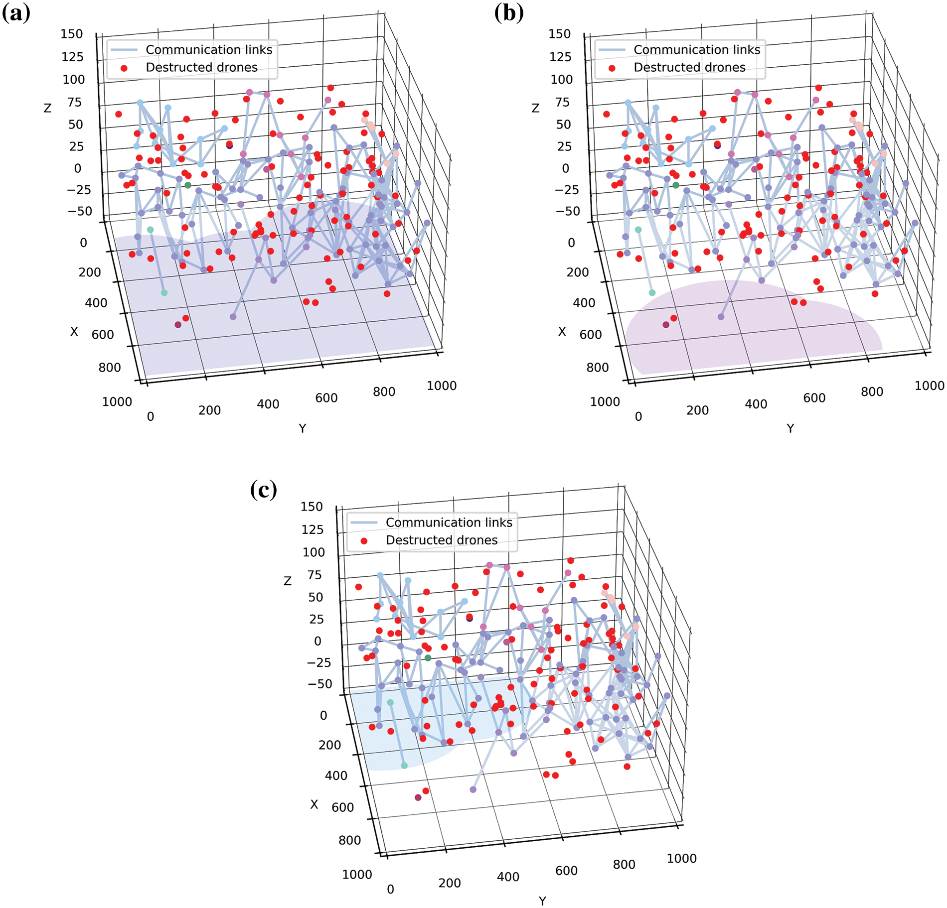
Figure 7: The coverage area of the initial swarm network after a certain destruction. (a) The coverage area of the maximal component of the network; (b) The coverage area of the second largest component of the network; (c) The coverage area of the third largest component of the network. The red dot represents the destructed drones

To study the performance of our method, we simulate the process of network connectivity recovery under single and continuous destructions, and compared the performance with SIDR [15], CM-MGCM [18], and CEN [18]. To conduct the experiments, the AMD Ryzen 7 5800H processor with Radeon Graphics is exploited. For connectivity verification, our main concern is to keep the entire network connected. Thus, we use the connected time step ratio as the evaluation measure for connectivity recovery. For coverage recovery verification, the resilience can be represented by the average network coverage performance R in a certain time slot based on (6) and (7), which can be represented as follows:

R=1Ts∑t0t0+Ts1M∑k=1M|∪i=1|𝒱tk|Bt,k(i)|/L2,(24)

where Ts is the time slot length, t0 is the beginning time, M is the number of connected components, and |𝒱tk| is the number of nodes within the k-th connected component.

Fig. 8 shows the different trajectories and coverage areas of the drones during a certain recovery process with TAGAT and CEN. It can be seen that the flight trajectory with TAGAT is not only simply moving toward the center of the group but also can achieve coverage recovery.

Figure 8: The recovery process of drones after a certain destruction. (a) Trajectories when drones fly to the target locations with TAGAT; (b) Trajectories when drones fly to the center of their positions directly, i.e., with the CEN; (c) Coverage area when drones fly to the target locations with the TAGAT; (d) Coverage area when flying to the target locations with CEN

4.1 Effect of the Proposed Framework on Network Connectivity Recovery

As shown in Fig. 9, we randomly destroy several nodes in the network from 15 to 135. In Figs. 9a–9c, we show the number of network clusters changes when the number of destructed drones is 15, 60, and 105, respectively. Figs. 9a–9c show the number of network clusters that changes with time under different numbers of destructed drones. When the number of damages is equal to 15, the performance of the TAGAT is similar to that of the CR-MGCM. Although the CR-MGCM has the best performance in the above cases, with the number of destructed drones increasing, the performance of the CR-MGCM obviously decreases. In contrast, when the number of damages is greater than 15, the TAGAT shows significantly better performance than the existing algorithms.

Figure 9: The results and comparisons between connected time step ratios with different algorithms. (a) The number of network clusters changes with time when the number of destructed drones is 15; (b) The number of network clusters changes with time when the number of destructed drones is 75; (c) The number of network clusters changes with time when the number of destructed drones is 135; (d) The connected time step ratio under different number of destructed drones with different algorithms

In Fig. 9d, we calculate the ratio of time T required for full recovery to the total time interval T*, and here set the T* = 300. Fig. 9d specifies the average of the connected time step ratio under different numbers of destructed drones with different algorithms. When the number of destructed drones varies from 15 to 135, the average results of the TAGAT are greater than those of the other three algorithms, i.e., the TAGAT algorithm can recover network connectivity faster. As shown in Fig. 9d, the connected time step ratio of TAGAT when the number of damages is greater than 15 is the highest, and the average result is improved by 17.92% compared with CR-MGCM.

As shown in Fig. 10, we simulate multiple destructions using a fixed case to ensure the same effect on the network, with a total time duration set to 150. In Fig. 10a, the destructions happen at times t = 10, t = 30, t = 100, and the number of destructions was 50, 10, and 10, respectively. It can be seen that after each destruction, the TAGAT can quickly recover network connectivity. Although with the CR-MGCM and the CEN, the network was not segmented after the third destruction, the recovery time of the above two algorithms was still too long after the first and second destruction. Thus, in terms of total connected time, the TAGAT maintains the network connected for the longest time. In Fig. 10b, the average and median connected time step ratios are higher than other algorithms regardless of the length of the time slot. Furthermore, with more destructions happening, the more TAGAT outperforms other algorithms.

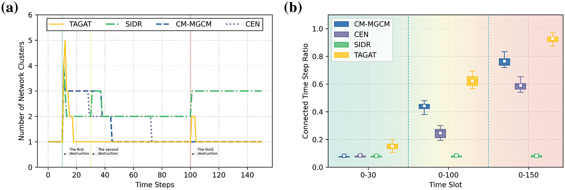
Figure 10: The results of connectivity with different algorithms under a certain case of three destructions. (a) The number of network clusters vs. time steps under a certain case of three destructions; (b) The distribution of the connected time step ratio with different algorithms in different time slots

4.2 Effect of the Proposed Framework on Network Coverage Recovery

To validate the effectiveness of the proposed method in coverage recovery, we also simulate the process of network connectivity recovery under single and continuous destructions and calculate the network resilience with different algorithms. As shown in Figs. 11a–11c, with the same experiment settings, the distribution of the network resilience under different numbers of destructed drones with different algorithms is similar to the results on connectivity. When the number of damages is more than 15, the coverage performance of the TAGAT is better than that of the CR-MGCM. With the number of destructed drones increasing, the gap between the coverage performances of TAGAT and CR-MGCM obviously increases. In Fig. 11d, the network resilience of TAGAT when the number of damages is greater than 15 is also the highest, and the average result is improved by 16.96% compared with CR-MGCM.

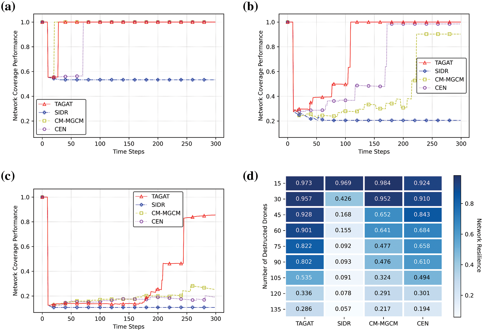
Figure 11: The results and comparisons between network resilience with different algorithms. (a) The network coverage performance changes with time when the number of destructed drones is 15; (b) The network coverage performance changes with time when the number of destructed drones is 75; (c) The network coverage performance changes with time when the number of destructed drones is 135; (d) The network resilience under different numbers of destructed drones with different algorithms

Fig. 12 presents the changes in coverage performance during the process of recovering network coverage. In Fig. 12a, it can be seen that the TAGAT, the CM-MGCM, and the CEN can all recover network coverage, but the SIDR is difficult to achieve. The TAGAT can recover network coverage faster compared to the CM-MGCM and the CEN, thereby achieving resilient network coverage. In Fig. 12b, the average and median resilience of the network with the TAGAT are stronger than other algorithms. With the length of time slot increases, TAGAT has better performance than other algorithms.

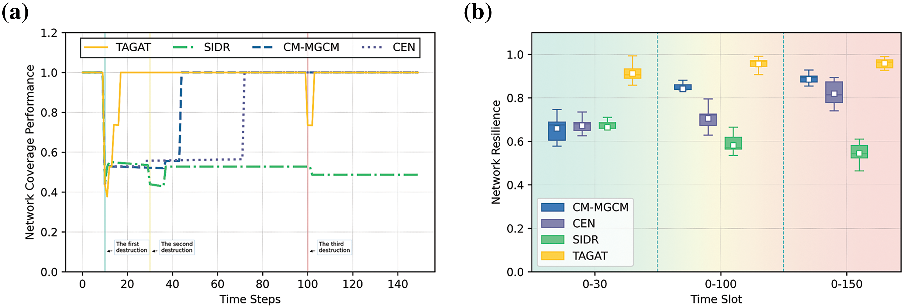
Figure 12: The results of coverage with different algorithms under a certain case of three destructions. (a) The network coverage performance vs. time steps under a certain case of three destructions; (b) The distribution of network resilience with different algorithms in different time slots

4.3 Ablation Study

Furthermore, to explicitly illustrate the contributions of the above improvements in performance enhancement, we perform the ablation study by creating different TAGAT variants, replacing one model component each time while keeping the rest unchanged, i.e., No-LossCoefficient, No-SructureImportance, and No-TemporalAggregationGraph.

In Fig. 13, the ablation study on network connectivity and network coverage is shown. We note that TAGAT is superior to all TAGAT variants without the above improvements, for both the network connectivity and network coverage, which shows that the above improvements help improve the ability to recover connectivity and coverage. The results indicate that all our improvement points help to improve the performances after various numbers of destructions, among which the temporal aggregation graph contributes the most, and the loss coefficient contributes the least, as the results demonstrate the worst ability to recover connectivity and coverage when TAGAT without the temporal aggregation graph unit.

Figure 13: The results of the ablation study. (a) Ablation results in the network connectivity; (b) Ablation results in the network coverage

5  Conclusions

In this paper, we studied the connectivity and coverage recovery problem of FANET with changing nodes and edges under destructions. Specifically, we proposed a recovery model considering both the coverage and the connectivity based on engineering resilience. Then, we incorporated a temporal aggregation graph generating method into GAT. Simulation results showed that the proposed algorithms can facilitate rapid recovery of the connectivity and coverage more effectively compared to the existing algorithms. In addition, by the ablation study, we quantify the contributions of each different improvement, indicating the temporal aggregation graph contributes the most to the performance of the rapid recovery.

In this study, the network we focused on is homogeneous, i.e., each drone plays the same role and shares the same power limit in the network. However, the scenarios of heterogeneous units jointly executing various missions began to appear in reality recently. In the future, we may extend our work to the heterogeneous FANET.

Acknowledgement: The authors would like to thank Jie Li and Chuhan Zhou for their assistances during writing.

Funding Statement: This research was funded by the National Natural Science Foundation of China (NNSFC) (Grant Nos. 72001213 and 72301292), the National Social Science Fund of China (Grant No. 19BGL297), and the Basic Research Program of Natural Science in Shaanxi Province (Grant No. 2021JQ-369).

Author Contributions: The authors confirm contribution to the paper as follows: Conceptualization, Zhijun Guo and Yun Sun; methodology, Ying Wang; software, Zhijun Guo and Chaoqi Fu; validation, Ying Wang and Jilong Zhong; formal analysis, Zhijun Guo and Yun Sun; writing—original draft preparation, Zhijun Guo; writing—review and editing, Jilong Zhong and Yun Sun. All authors have read and agreed to the published version of the manuscript.

Availability of Data and Materials: Due to the nature of this research, participants of this study did not agree for their data to be shared publicly, so supporting data is not available.

Conflicts of Interest: The authors declare that they have no known competing financial interests or personal relationships that could have appeared to influence the work reported in this paper.

References

1. H. Wang, H. Zhao, J. Zhang, D. Ma, J. Li and J. Wei, “Survey on unmanned aerial vehicle networks: A cyber physical system perspective,” IEEE Commun. Surv. Tutorials, vol. 22, no. 2, pp. 1027–1070, 2020. doi: 10.1109/COMST.2019.2962207. [Google Scholar] [CrossRef]

2. L. Gupta, R. Jain, and G. Vaszkun, “Survey of important issues in UAV communication networks,” IEEE Commun. Surv. Tutorials, vol. 18, no. 2, pp. 1123–1152, 2016. doi: 10.1109/COMST.2015.2495297. [Google Scholar] [CrossRef]

3. S. Hayat, E. Yanmaz, and R. Muzaffar, “Survey on unmanned aerial vehicle networks for civil applications: A communications viewpoint,” IEEE Commun. Surv. Tutorials, vol. 18, no. 4, pp. 2624–2661, 2016. doi: 10.1109/COMST.2016.2560343. [Google Scholar] [CrossRef]

4. A. Chriki, H. Touati, H. Snoussi, and F. Kamoun, “FANET: Communication, mobility models and security issues,” Comput. Netw., vol. 12, no. 9, pp. 163, 2019. doi: 10.1016/j.comnet.2019.106877. [Google Scholar] [CrossRef]

5. A. I. Hentati and L. C. Fourati, “Comprehensive survey of UAVs communication networks,” Comput. Stand. Interf., vol. 3, no. 3, pp. 72, 2020. doi: 10.1016/j.csi.2020.103451. [Google Scholar] [CrossRef]

6. P. Holme and J. Saramäki, “Temporal networks,” Phy. Rep., vol. 519, no. 3, pp. 97–125, 2012. doi: 10.1016/j.physrep.2012.03.001. [Google Scholar] [CrossRef]

7. S. Scellato, I. Leontiadis, C. Mascolo, P. Basu, and M. Zafer, “Evaluating temporal robustness of mobile networks,” IEEE Trans. Mob. Comput., vol. 12, no. 1, pp. 105–117, 2013. doi: 10.1109/TMC.2011.248. [Google Scholar] [CrossRef]

8. G. Bai, Y. Li, Y. Fang, Y. A. Zhang, and J. Tao, “Network approach for resilience evaluation of a UAV swarm by considering communication limits,” Reliab. Eng. Syst. Safety, vol. 11, no. 4, pp. 193, 2020. doi: 10.1016/j.ress.2019.106602. [Google Scholar] [CrossRef]

9. K. Liu, J. Zhong, G. Bai, and Y. Yang, “A complex networks approach for reliability evaluation of swarm systems under malicious attacks,” IEEE Access, vol. 8, pp. 81209–81219, 2020. doi: 10.1109/ACCESS.2020.2991211. [Google Scholar] [CrossRef]

10. A. Pananjady, V. K. Bagaria, and R. Vaze, “Optimally approximating the coverage lifetime of wireless sensor networks,” IEEE/ACM Trans. Netw., vol. 25, no. 1, pp. 98–111, 2017. doi: 10.1109/TNET.2016.2574563. [Google Scholar] [CrossRef]

11. M. Mozaffari, W. Saad, M. Bennis, and M. Debbah, “Efficient deployment of multiple unmanned aerial vehicles for optimal wireless coverage,” IEEE Commun. Lett., vol. 20, no. 8, pp. 1647–1650, 2016. doi: 10.1109/LCOMM.2016.2578312. [Google Scholar] [CrossRef]

12. X. Bai, Z. Yun, D. Xuan, W. Jia, and W. Zhao, “Pattern mutation in wireless sensor deployment,” presented at the IEEE INFOCOM 2010, San Diego, CA, USA, 2010, pp. 1–9. [Google Scholar]

13. M. Li, Z. Li, and A. V. Vasilakos, “A survey on topology control in wireless sensor networks: Taxonomy comparative study, and open issues,” in Proc. IEEE, vol. 101, pp. 2538–2557, 2013. [Google Scholar]

14. K. P. Sharma and T. P. Sharma, “ZBFR: Zone based failure recovery in WSNs by utilizing mobility and coverage overlapping,” Wirel. Netw., vol. 23, no. 7, pp. 2263–2280, 2016. doi: 10.1007/s11276-016-1291-2. [Google Scholar] [CrossRef]

15. M. Chen, H. Wang, C. Y. Chang, and X. Wei, “SIDR: A swarm intelligence-based damage-resilient mechanism for UAV swarm networks,” IEEE Access, vol. 8, pp. 77089–77105, 2020. doi: 10.1109/ACCESS.2020.2989614. [Google Scholar] [CrossRef]

16. X. Qi, P. Yuan, Q. Zhang, and Z. Yang, “CDS-based topology control in FANETs via power and position optimization,” IEEE Wirel. Commun. Lett., vol. 9, no. 12, pp. 2015–2019, 2020. doi: 10.1109/LWC.2020.3009666. [Google Scholar] [CrossRef]

17. J. Guo and C. Yang, “Learning power allocation for multi-cell-multi-user systems with heterogeneous graph neural networks,” IEEE Trans. Wirel. Commun., vol. 21, no. 2, pp. 884–897, 2022. doi: 10.1109/TWC.2021.3100133. [Google Scholar] [CrossRef]

18. Z. Mou, F. Gao, J. Liu, and Q. Wu, “Resilient UAV swarm communications with graph convolutional neural network,” IEEE J. Selected Areas Commun., vol. 40, pp. 393–411, 2022. [Google Scholar]

19. Z. Mou, Y. Zhang, F. Gao, H. Wang, T. Zhang and Z. Han, “Deep reinforcement learning based three-dimensional area coverage with UAV swarm,” IEEE J. Sel. Areas Commun., vol. 39, no. 10, pp. 3160–3176, 2021. doi: 10.1109/JSAC.2021.3088718. [Google Scholar] [CrossRef]

20. C. Zhang, W. Yao, Y. Zuo, H. Wang, and C. Zhang, “Robust multiple unmanned aerial vehicle network design in a dense obstacle environment,” Drones, vol. 7, no. 8, pp. 508–526, 2023. doi: 10.3390/drones7080506. [Google Scholar] [CrossRef]

21. J. Lyu and R. Zhang, “Network-connected UAV: 3-D system modeling and coverage performance analysis,” IEEE Internet Things J., vol. 6, no. 4, pp. 7048–7060, 2019. doi: 10.1109/JIOT.2019.2913887. [Google Scholar] [CrossRef]

22. F. Chung, “The laplacian and eigenvalues,” in Spectral Graph Theory (CBMS Regional Conference Series in Mathematics), 1st ed. Providence, Rhode Island, USA, 1996, vol. 1, pp. 2–6. [Google Scholar]

23. S. Hosseini, K. Barker, and J. E. Ramirez-Marquez, “A review of definitions and measures of system resilience,” Reliab. Eng. Syst. Safety, vol. 145, no. 12, pp. 47–61, 2016. doi: 10.1016/j.ress.2015.08.006. [Google Scholar] [CrossRef]

24. C. Cangea, P. Veličković, N. Jovanović, T. Kipf, and P. Liò, “Towards sparse hierarchical graph classifiers,” arXiv:1811.01287, 2018. [Google Scholar]

25. S. Ruder, “An overview of gradient descent optimization algorithms,” arXiv:1609.04747, 2016. [Google Scholar]

26. W. L. Hamilton, R. Ying, and J. Leskovec, “Inductive representation learning on large graphs,” in Proc. 31st Int. Conf. Neur. Inf. Process. Syst., Long Beach, California, USA, 2017, pp. 1025–1035. [Google Scholar]

27. Y. Xiao, H. Shao, M. Feng, T. Han, J. Wan and B. Liu, “Towards trustworthy rotating machinery fault diagnosis via attention uncertainty in transformer,” J. Manuf. Syst., vol. 70, no. 9, pp. 186–201, 2023. doi: 10.1016/j.jmsy.2023.07.012. [Google Scholar] [CrossRef]

28. S. Yan, H. Shao, J. Wang, X. Zheng, and B. Liu, “LiConvFormer: A lightweight fault diagnosis framework using separable multiscale convolution and broadcast self-attention,” Expert. Syst. App., vol. 237, no. 1, pp. 1213–1238, 2024. doi: 10.1016/j.eswa.2023.121338. [Google Scholar] [CrossRef]

29. Z. Liu and J. Zhou, “Graph attention networks, Introduction to graph neural networks,” Synth. Lect. Artif. Intell. Mach. Learn., vol. 14, pp. 1–127, 2020. [Google Scholar]

30. S. Brody, U. Alon, and E. Yahav, “How attentive are graph attention networks?,” arXiv:2105.14491, 2021. [Google Scholar]

31. A. Barabási, “Network robustness,” in Network Science, 1st ed. UK: Cambridge University Press, 2016, pp. 5–8. [Google Scholar]

32. D. D. Woods, “Four concepts for resilience and the implications for the future of resilience engineering,” Reliab. Eng. Syst. Safety, vol. 141, no. 1, pp. 5–9, 2015. doi: 10.1016/j.ress.2015.03.018. [Google Scholar] [CrossRef]