
 Submit a Paper
 Propose a Special lssue
 Open Access
ARTICLE

A Heuristic Radiomics Feature Selection Method Based on Frequency Iteration and Multi-Supervised Training Mode
1 School of Computer, Hunan University of Technology, Zhuzhou, 412007, China
2 Hunan Key Laboratory of Intelligent Information Perception and Processing Technology, Zhuzhou, 412007, China
* Corresponding Author: Yanhui Zhu. Email:
(This article belongs to the Special Issue: Recent Advances in Ensemble Framework of Meta-heuristics and Machine Learning: Methods and Applications)
Computers, Materials & Continua 2024, 79(2), 2277-2293. https://doi.org/10.32604/cmc.2024.047989
Received 24 November 2023; Accepted 14 March 2024; Issue published 15 May 2024
 View Full Text
 Download PDF
Abstract
Radiomics is a non-invasive method for extracting quantitative and higher-dimensional features from medical images for diagnosis. It has received great attention due to its huge application prospects in recent years. We can know that the number of features selected by the existing radiomics feature selection methods is basically about ten. In this paper, a heuristic feature selection method based on frequency iteration and multiple supervised training mode is proposed. Based on the combination between features, it decomposes all features layer by layer to select the optimal features for each layer, then fuses the optimal features to form a local optimal group layer by layer and iterates to the global optimal combination finally. Compared with the current method with the best prediction performance in the three data sets, this method proposed in this paper can reduce the number of features from about ten to about three without losing classification accuracy and even significantly improving classification accuracy. The proposed method has better interpretability and generalization ability, which gives it great potential in the feature selection of radiomics.Keywords
As a novel, economical and convenient non-invasive technology [1], radiomics aims to extract quantitative and higher dimensional data from digital biomedical images to promote the comprehensive exploration of medical image information and changes in information [2]. The operations of radiomics are intuitive and have good interpretability [3]. In addition, it is closely linked with artificial intelligence, and has great potential to achieve standardization and automation to greatly improve the efficiency of diagnosis [4]. So, it has received much attention in the field of medical diagnosis in recent years [5].
The radiomics pipeline of modelling with manually defined features and deep learning. For Modelling with manually defined features, it includes the main steps: Data acquisition and preprocessing, tumor segmentation, feature extraction and selection, and modeling. For deep learning, it is an end-to-end method without separate steps of feature extraction, feature selection and modelling. Trained models from both two methods should be validated with a new dataset and then could be applied. The standard radiomics process is shown in Fig. 1.

Figure 1: The standard radiomics process. Abbreviations: AUC, area under the receiver operating characteristic curve; C-index, concordance index; DFS, disease-free survival; PFS, progression-free survival; OS, overall survival. Reprinted with permission from Liu et al. [6]
Radiomics features typically comprise a small number of components that are easily understood by people, such as tumor dimensions, shape, and margin characteristics. However, they also encompass a multitude of components that are not readily understandable to individuals, including enhancement texture, quantifications of kinetic curves, and enhancement-variance kinetics [7]. Despite their complexity, all these components reflect certain characteristics of the image. However, the total amount of these features is huge, which is also a common problem in the application of artificial intelligence in the medical field, namely low computational efficiency and performance degradation caused by high-dimensional data [8]. Therefore, it is necessary to streamline the data, generally using two methods: Feature reduction and feature selection [9].
Feature dimensionality reduction is a method of removing noise and redundant features by projecting the original high-dimensional data onto a low-dimensional subspace [10]. However, features mapped to subspaces can lose their original position information, resulting in the loss of many physical meanings, which limits their application in many fields, such as gene and protein analysis [11], because a crucial factor in the clinical application of artificial intelligence is the interpretability of the model [12]. Feature selection is an effort to select feature subsets from high-dimensional data to improve data density, reduce noise features, and alleviate overfitting, high computational consumption, and low-performance issues in practice [13]. Therefore, feature selection and dimensionality reduction are crucial for data processing, and feature selection does not alter the features themselves, making it more interpretable than feature dimensionality reduction [14]. For this reason, feature selection methods are generally used in radiomics [15].
However, currently in the field of radiomics, there are some common problems with existing feature selection methods. Firstly, most of the selected features are 5 or more, and secondly, the selected features cannot achieve satisfactory results on models with good solvability, such as on decision trees. This study aims to solve this problem.
This paper proposes a new heuristic hybrid method based on the wrapping method and embedding method. It takes the wrapping method as the core to ensure accuracy, uses an embedding method for primary selection to reduce the search space, and is guided by heuristic ideas inspired by chemical reactions between substances to accelerate convergence. This method was validated in radiomics datasets from three different fields.
The remaining parts of this study were conducted in the following manner: Section 2 gives the related work on the feature selection methods. Section 3 involves the dataset and its partitioning used in this study. A detailed explanation of the algorithm proposed in this article is provided in Section 4. Section 5 provides a detailed introduction to the experimental design of this method. Section 6 provides the experimental results and an analysis of the experimental results. Section 7 contains discussions, while Section 8 contains conclusions and future work.
According to evaluation criteria, existing feature selection methods can be divided into four categories: 1) Wrapping method; 2) Filtration method; 3) Embedding method; and 4) Hybrid method [16]; The wrapping method uses the role of features in the classification model (F-M) as a selection factor, continuously selecting feature subsets from the initial feature set, evaluating the subsets based on the performance of the model, until the best subset is selected, such as recursive feature elimination (RFE) [17] and genetic algorithm (GA) [18]. The filtering method usually uses certain statistical measures (such as t-test [19] and mutual information [20]). Embedded methods mainly use the interdependence relationship (F-F) between features as a selection factor and feature selection as part of the training process, such as Least absolute shrinkage and selection operator (LASSO) [21] and Boruta [22]. Each single method has its own significant advantages and disadvantages [23]. For example, filtering methods usually operate faster than wrapping methods. However, compared to wrapping methods, the main problem of filtering methods is that they only consider individual features and ignore the combination characteristics between features, so they often cannot achieve higher classification accuracy [24]. The wrapping rule has problems with slow training speed and easy overfitting on small samples [25]. Embedded methods also have the disadvantage of not being suitable for high-dimensional data and having poor universality [26].
Hybrid methods combine multiple methods, which can significantly reduce the disadvantages of each single method while maintaining its advantages [27,28]. For example, a hybrid method is composed of the filtering method and wrapping method, in which the filtering method first removes irrelevant features, and the wrapping method selects important features from a candidate subset. Combining multiple basic methods can help one better adapt to different tasks, playing a certain complementary role in advantages [29].
In addition, there is an important heuristic idea that is inspired by various natural phenomena, aiming to apply the principles behind certain natural phenomena to feature selection methods. The application of this idea has achieved great success in recent years [30,31]. According to their sources of inspiration, some of them are inspired by biological phenomena such as natural evolution. In contrast, others imitate the social behavior of animals in cattle and sheep herds [32–34] or imitate some physical laws in nature [35], as well as inspired by human invention activities [36].
This study is influenced by the characteristics of chemical reactions in the field of chemistry, treating a group of features as a single chemical substance. If the characteristics of different groups are combined to improve accuracy, they are considered to have undergone a binding reaction. The overall view is that the higher the score of the combination and the fewer elements, the easier it is to react and bind more tightly. Adopting this principle can, to some extent, avoid the occurrence of extreme situations where only strong features are combined with each other.
3 Dataset Introduction and Partitioning
To verify the universality of the proposed radiomics feature selection method in different radiomics tasks, this study collected open-access datasets from three different fields of radiomics. Table 1 lists the detailed information of each dataset, including the corresponding dataset, the category and number of patients, and the number of features. Each dataset used in this study was approved by the respective institutional ethics review committee, and the data collection process complied with relevant guidelines and regulations. In addition, this experiment only focuses on selecting the most important feature among the radiomics features extracted by the patient, so the data directly used is the radiomics feature data that has already been extracted from the imaging data.
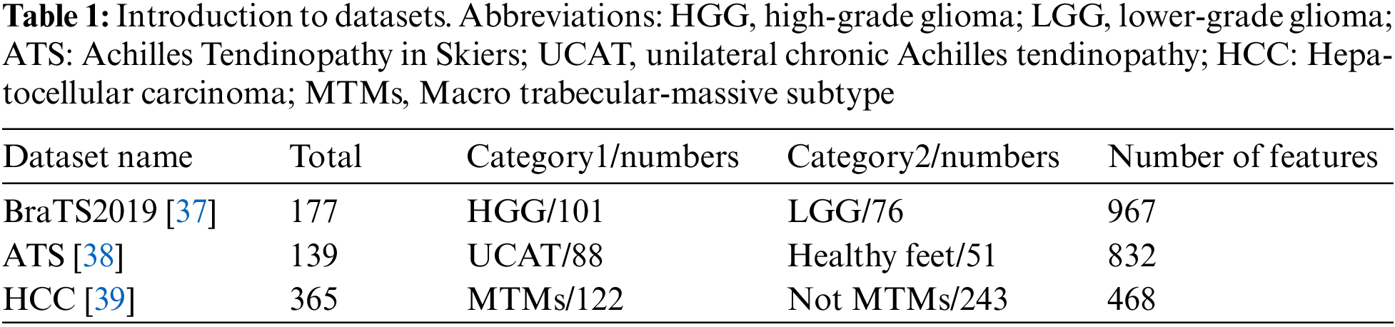
The specific representation of radiomics feature data is represented by numerical values, and each feature is represented by a numerical value. The calculation of these feature values can be obtained through a series of manually set statistical quantification indicators or through deep learning. These data look like a table filled with numbers, where rows represent the samples and columns represent the radiomics characteristics of the samples.
Divide each dataset into three types according to the size of the training set: Small, medium, and large, namely Data_A. Data_B. Data_C. This way, we can compare and determine which method is more effective when the sample size is small. In addition, in order to make the comparison of their generalization ability more reliable, we divided the test set into two parts. Because two test sets may have one high and one low, and only one test set would not reflect such a difference, dividing the test set into two parts greatly avoids this problem. If the sample size is too small, there is no need for further division. Table 2 provides a detailed description of the partitioning results.

4.1 Multiple Supervised Training Mode
To improve the generalization ability of the selected features in this method, this paper proposes a multi-supervised training mode. Divide the training data into several subsets and train each subset separately while other subsets participate in evaluating performance. The trained model uses the lowest score of the other subsets participating in the evaluation as the score of that subset, and ultimately uses the lowest score of all subsets as the final score. Fig. 2 shows the process of multi-supervised training mode. Algorithm 1 provides a detailed description of its implementation.

Figure 2: The process of multi-supervised training mode

4.2 Feature Selection Method Based on Frequency Iteration
This paper proposes a heuristic feature selection method based on frequency iteration to make the best use of the advantages of the wrapping method and the embedded method while avoiding their disadvantages as much as possible to achieve a good balance. First, the embedded method is used to conduct a preliminary selection of features to reduce the search space quickly. LASSO is the best way to match. On the one hand, LASSO can flexibly control the number of pre-selected features, and the features selected by LASSO have good noncollinearity [40].
The basic operation of the heuristic feature selection method based on frequency iteration is decomposition and refusion. The total feature combination is divided into a series of small feature combinations, and then the local optimal combination is generated from the small feature combinations. These local optimal combinations are fused, and then the operation is repeated until the specified number of features are iterated. The decomposition method can change the exponential increase in search complexity caused by the linear increase in the number of features to a linear increase [41], greatly reducing the complexity of the wrapping method. For each segment, the refusion can largely offset the data isolation effect forced by data segmentation.
The generation of local optimal combinations adopts the idea of dichotomy, which always follows the principle of pairwise combination. If the accuracy of the combination improves, a new combination is generated. Otherwise, the one with the highest accuracy is selected from the old combination.
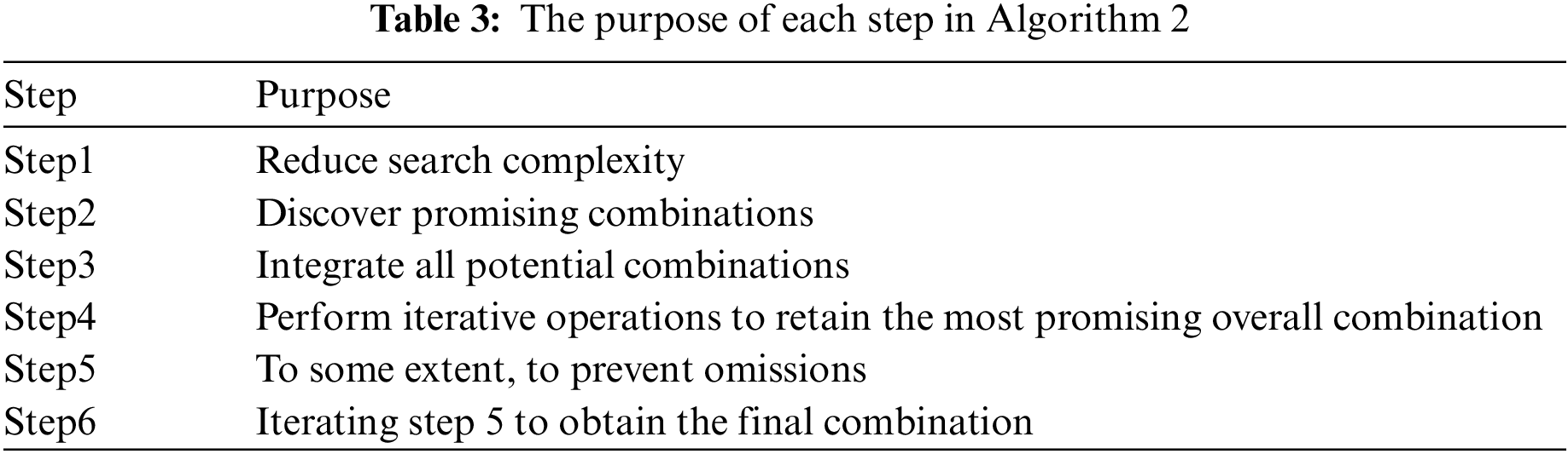
This method can largely take into account weak (but important) predictive factors highly correlated with strong predictive factors [42] rather than tending towards combinations between strong features, as such combinations may actually have poorer results, and sometimes the combination between weak features or strong and weak features may have better results [43]. This method largely avoids extremism, greatly increasing the probability of various potential good combinations meeting. Algorithm 2 summarizes the basic process of this scheme. Fig. 3 shows an example of the overall process of this method. Table 3 summarizes the objectives that each step of Algorithm 2 aims to achieve.

Figure 3: An example of the overall process of this method

4.3 Algorithm Complexity Analysis
4.3.1 Time Complexity Analysis
In Algorithm 1, two loops are nested, and each loop performs a traversal with a time complexity of
In Algorithm 2, the main consideration is the time complexity of iteratively executing steps 1, 2, and 3, which are related to the number of features S contained in the shard and the initial number of features
4.3.2 Spatial Complexity Analysis
Algorithm 1 uses two lists, both of which have a spatial complexity of
Algorithm 2 requires a pairwise combination of elements in each shard, and the amount of data stored in each shard is
5.1 Selection of Basic Classifiers
When using the wrap method for feature selection, it is necessary to specify a basic classifier. In the feature selection of radiomics, the classification accuracy and speed of support vector machine (SVM) in binary classification problems are excellent, and the comprehensive performance is better than other classifiers. Therefore, in this experiment, SVM is used as the basic classifier when using the wrapping method for feature selection.
In order to compare the effects of the features selected by different methods, two basic classifiers, SVM and decision tree (DT), are used, respectively. Because SVM can best reflect the highest accuracy of the selected features, and tree-based classifier has the best interpretability [44]. We can intuitively understand the accuracy (ACC), interpretability, and generalization potential of the selected features through these two basic classifiers to test the effect of the features selected by different methods. The hyperparameters of the two basic classifiers are automatically determined by grid search, and both are subject to fivefold cross-validation.
5.2 Comparison Methods, Parameter Settings, and Evaluation Criteria
Regarding the most advanced feature selection methods in radiomics, Demircioğlu evaluated 29 feature selection algorithms and ten classifiers on ten publicly available radiomics datasets in a study on radiomics feature selection methods in July 2022 [15]. His research shows that different feature selection methods vary greatly in training time, stability, and similarity, but no method consistently outperforms another in predictive performance. However, overall, LASSO performs the best in analyzing predictive performance among all feature selection methods. Therefore, if compared comprehensively, it can be said that LASSO is the best method among radiomics feature selection methods. In the experiment of validating the algorithm, our method was compared with LASSO.
For the parameters of this method, N in Algorithm 1 is set to 5, and size and Q in Algorithm 2 are both set to 6. For LASSO parameters, penalty items λ determine the sparsity of the selected feature, and the effect of different sparsity is different in different tasks. To maximize the effect of LASSO, compare the effect of sparse and dense states, respectively, and select the best one λ, then select the best five and the best ten features respectively for comparison. The specific evaluation indicators and standards are shown in Table 4.

6 Experimental Results and Analysis
According to the data division in Table 2, the experiment compares the performance of our method and LASSO on three datasets. The visualization of the experimental results is shown in Figs. 4–6. The calculated p values in each experiment are shown in Table 5. The red line in the figure represents our method, the blue line represents the performance of LASSO finally selecting the five best features, the black line represents the performance of LASSO finally selecting the ten best features, and the solid line represents the performance of SVM for prediction, The dotted line indicates that the DT is used for prediction. The name of the horizontal axis represents whether it is a training or testing set, and the number represents the number of samples in the training or testing set. In the bar chart, yellow represents our method, green represents LASSO’s final selection of the best 5 features, and purple represents LASSO’s final selection of the best 10 features. The number inside the column is the name code of the feature, which refers to the column of features in the sample. The number above the column represents the final number of selected features.

Figure 4: Performance of the algorithm on the BraTS2019 dataset
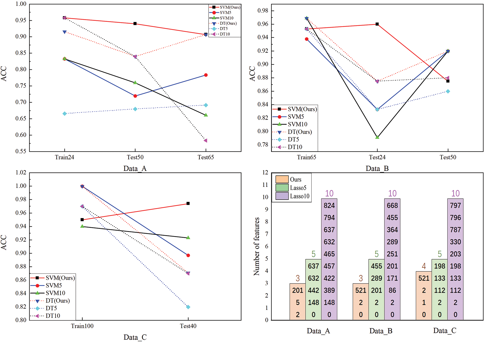
Figure 5: Performance of the algorithm on the ATS dataset


Figure 6: Performance of the algorithm on the HCC dataset

In terms of accuracy, under the same classifier, our method performs significantly better than LASSO in the experiments represented in Figs. 4 and 5, while performing similarly to LASSO in the experiments represented in Fig. 6. From the number of features selected in the final feature combination of our method, it can be seen that our method outperforms LASSO significantly in the experiments represented by Figs. 4 and 6, while slightly better than LASSO in the experiments represented by Fig. 5. From the perspective of classifiers, whether choosing SVM or DT, our method outperforms LASSO significantly in the experiments represented in Figs. 4 and 5, and performs equally on both classifiers. However, LASSO’s performance on DT is far inferior to SVM, indicating that our method has better interpretability. From the fluctuations in the results of different methods in datasets with different distributions, it can be seen that our method has smaller fluctuations, better stability, and better generalization ability. From Table 5, it can be seen from the analysis of the overall representative p values of the selected feature combinations in each experiment that, except for the experiment represented in Fig. 6, our method’s final selected feature combination has a significantly stronger overall association strength for classification than LASSO, with a very high confidence level.
Through the analysis of the experiment, it can be known that the main advantage of our method is that it can reduce the number of ultimately selected features, and reducing the number of features can reduce computational costs, memory requirements, and model complexity to improve computational efficiency, especially in large-scale datasets and resource-constrained environments. In addition, a decrease in the number of features means a reduction in noisy and redundant data, which can effectively improve the model’s generalization ability. At the same time, selecting fewer features can make the model easier to understand and interpret, enhance insight into the relationship between features and models, and improve the interpretability of the model.
Although reducing the number of features greatly helps with the interpretability of the model, the most helpful aspect is that the selected features can also perform well on the DT. DT has good interpretability because its model structure is intuitive and has strong visualization ability, which can clearly display the importance of features and decision rules, enabling people to understand the model’s decision-making process intuitively. In addition, DT can also determine the relative importance of each feature through feature importance assessment, further providing the ability to interpret the model.
As for the improvement of the model’s generalization ability, in addition to reducing the number of ultimately selected features, the most crucial factor is the use of a multi-supervised training mode, which eliminates combinations with insufficient generalization ability through multiple supervision, ultimately ensuring the model’s generalization ability.
A major difficulty in applying AI in the medical field is the interpretability of AI decision-making. Although many deep learning methods have made great progress in accuracy, at this stage, deep learning still lacks interpretability in many problems, which greatly hinders the clinical application of AI technology [45]. A fundamental reason for the poor interpretability of artificial intelligence is that its decision-making parameters are huge, and it is difficult for people to find an intuitive and explanatory basis from such huge parameters [46]. Reducing the dimension of data is undoubtedly of great help to solvability. This method can greatly reduce the number of features on which decisions are based and is conducive to the characteristic engineering and statistical modeling of radiomics [47], which will greatly help the application of radiomics in practical medical treatment.
Another major challenge in applying artificial intelligence in the medical field is the scarcity of data resources. Deep learning is currently the mainstream artificial intelligence method, which requires feeding a large amount of high-quality data to achieve good accuracy [48]. This significantly limits the application of artificial intelligence in the medical application field. Even some machine learning methods that do not require much sample size, such as Lasso’s methods, may have insufficient generalization ability when the sample size is small [40]. The features extracted by the method in this article have strong generalization ability, and even in a relatively small sample set, representative and strong generalization ability feature combinations can be extracted.
Because this is a heuristic algorithm, it is inevitably sensitive to the initial values of some parameters, such as the size of each shard, which leads to different initial values and different results. There are two solutions to this situation to obtain good and stable results. Firstly, a small-scale grid search can be performed for the value of S. Additionally, multiple tests can be conducted for the same value of S to select the optimal result.
In addition, because the process of this method is segmented and converges layer by layer, there may also be a so-called “nesting effect”, as the selected or deleted features cannot be deleted or selected in the later stage [49]. So, a certain segment, may contain features that make another segment more effective, but being deleted in that segment makes it impossible to meet other segments. Although all missing elements will be gradually investigated in the end, this can only add to the icing on the cake. In addition, because this method is essentially a heuristic search method, it inevitably has the problem of running longer than other methods.
In order to overcome the problem of the large number of features ultimately selected by existing radiomics feature selection methods, which is not conducive to the interpretability and generalization ability of the model, this paper comprehensively considers the advantages and disadvantages of various basic methods. To achieve a better balance between computational complexity and classification accuracy, a heuristic feature selection method based on frequency iteration and multiple supervised training modes is proposed. It takes the wrapping method as the core to ensure accuracy, the embedding method for initial selection to reduce the search space, and the heuristic idea as the guidance to accelerate convergence. Based on the combination effect between features, all features are decomposed layer by layer, and each layer is optimized segment by segment, and then the selected features are fused to form a local optimal group layer by layer, and finally iterate to approach the global optimal combination. In addition, to improve the generalization ability, a multiple supervision mode is proposed. The core is cross-training and cross-evaluation, with a small amount of training and many evaluations to ensure the model’s powerful generalization ability.
By comparing three different types of radiomics datasets, it was found that this method has great potential in radiomics feature extraction, effectively reducing the number of ultimately selected features. The selected features also have good performance in the decision tree, have good generalization ability and interpretability, and can be used as a method for radiomics feature extraction, our research contributions are summarized as follows:
(I) The exponential growth of the search complexity caused by the linear growth of the number of features in the wrapping method is transformed into linear growth through the divide-and-conquer idea.
(II) The heuristic idea inspired by chemical reactions, combined with the packaging method as the core of the local selection and refusion strategy, not only fully considers the possibility of different combinations during the iteration process, but also avoids the extreme tendency of only combining strong features with each other.
(III) The model’s generalization ability is greatly improved by using multiple supervised training mode.
(IV) By combining the wrapping and embedding methods, they avoid two extremes in accuracy and speed, thus achieving a good balance.
Although our method may not always perform well on all datasets, it does show great potential in reducing the number of selected features and improving the interpretability and generalization ability of the model. This can have a positive impact on the clinical application of radiomics.
In the future, we will conduct targeted performance optimization based on the limitations of this method. One possible direction is that because each segment of the method generates many combinations, these combinations may discover some rules through statistical analysis. If statistical learning methods such as the Bayesian theorem can be utilized to a certain extent to dynamically estimate the potential for different features or feature combinations to produce good results with other combinations, it will greatly reduce the probability of missing potential good combinations, thereby greatly improving the performance of the algorithm.
Acknowledgement: The authors would like to thank the anonymous reviewers and the editor for their valuable suggestions, which greatly contributed to the improved quality of this article.
Funding Statement: This work is supported by Major Project for New Generation of AI Grant No. 2018AAA0100400), and the Scientific Research Fund of Hunan Provincial Education Department, China (Grant Nos. 21A0350, 21C0439, 22A0408, 22A0414, 2022JJ30231, 22B0559), and the National Natural Science Foundation of Hunan Province, China (Grant No. 2022JJ50051).
Author Contributions: The authors confirm their contribution to the paper as follows: Study conception and design: Z. Zeng, A. Tang, Y. Zhu; data collection: A. Tang, Y. Zhu, S. Yi; analysis and interpretation of results: Z. Zeng, A. Tang, X. Yuan; draft manuscript preparation: A. Tang, S. Yi, X. Yuan. All authors reviewed the results and approved the final version of the manuscript.
Availability of Data and Materials: The data for this study is derived from open-source datasets. The BraTS2019 related dataset is accessible at https://www.med.upenn.edu/cbica/brats-2019/. The ATS dataset can be found on GitHub at the link https://GitHub.com/JZK00/Ultrasound-Image-Based-Radiomics. The link to the HCC dataset is https://GitHub.com/Zachary2017/HCC-Radiomics2022.
Conflicts of Interest: The authors declare that they have no conflicts of interest to report regarding the present study.
References
1. E. P. Huang et al., “Criteria for the translation of radiomics into clinically useful tests,” Nat. Rev. Clin. Oncol., vol. 20, no. 2, pp. 69–82, 2023. doi: 10.1038/s41571-022-00707-0. [Google Scholar] [PubMed] [CrossRef]
2. J. Guiot et al., “A review in radiomics: Making personalized medicine a reality via routine imaging,” Med. Res. Rev., vol. 42, no. 1, pp. 426–440, 2022. doi: 10.1002/med.21846. [Google Scholar] [PubMed] [CrossRef]
3. L. Dercle et al., “Artifificial intelligence and radiomics: Fundamentals, applications, and challenges in immunotherapy,” J. Immunother. Cancer, vol. 10, no. 9, pp. e005292, 2022. [Google Scholar] [PubMed]
4. C. J. Haug and J. M. Drazen, “Artifificial intelligence and machine learning in clinical medicine,” New Engl. J. Med., vol. 388, no. 13, pp. 1201–1208, 2023. doi: 10.1056/NEJMra2302038. [Google Scholar] [PubMed] [CrossRef]
5. K. Bera, N. Braman, A. Gupta, V. Velcheti, and A. Madabhushi, “Predicting cancer outcomes with radiomics and artifificial intelligence in radiology,” Nat. Rev. Clin. Oncol., vol. 19, no. 2, pp. 132–146, 2022. doi: 10.1038/s41571-021-00560-7. [Google Scholar] [PubMed] [CrossRef]
6. Z. Liu et al., “The applications of radiomics in precision diagnosis and treatment of oncology: Opportunities and challenges,” Theranostics, vol. 9, no. 5, pp. 1303–1322, 2019. doi: 10.7150/thno.30309. [Google Scholar] [PubMed] [CrossRef]
7. M. R. Tomaszewski and R. J. Gillies, “The biological meaning of radiomic features,” Radiology, vol. 298, no. 3, pp. 505–516, 2021. doi: 10.1148/radiol.2021202553. [Google Scholar] [PubMed] [CrossRef]
8. F. Nie, Z. Wang, R. Wang, and X. Li, “Submanifold-preserving discriminant analysis with an auto optimized graph,” IEEE Trans. Cybern., vol. 50, no. 8, pp. 3682–3695, 2019. doi: 10.1109/TCYB.2019.2910751. [Google Scholar] [PubMed] [CrossRef]
9. V. Berisha et al., “Digital medicine and the curse of dimensionality,” npj Digit. Med., vol. 4, no. 153, pp. 44, 2021. doi: 10.1038/s41746-021-00521-5. [Google Scholar] [PubMed] [CrossRef]
10. M. T. Islam and L. Xing, “A data-driven dimensionality reduction algorithm for the exploration of patterns in biomedical data,” Nat. Biomed. Eng., vol. 5, no. 6, pp. 624–635, 2021. doi: 10.1038/s41551-020-00635-3. [Google Scholar] [PubMed] [CrossRef]
11. X. Sun, Y. Liu, and L. An, “Ensemble dimensionality reduction and feature gene extraction for single-cell rna-seq data,” Nat. Commun., vol. 11, no. 1, pp. 5853, 2020. doi: 10.1038/s41467-020-19465-7. [Google Scholar] [PubMed] [CrossRef]
12. C. Combi et al., “A manifesto on explainability for artifificial intelligence in medicine,” Artif. Intell. Med., vol. 133, no. 4, pp. 102423, 2022. doi: 10.1016/j.artmed.2022.102423. [Google Scholar] [PubMed] [CrossRef]
13. Z. Wang, X. Xiao, and S. Rajasekaran, “Novel and effificient randomized algorithms for feature selection,” Big Data Min. Anal., vol. 3, no. 3, pp. 208–224, 2020. doi: 10.26599/BDMA.2020.9020005. [Google Scholar] [CrossRef]
14. V. Bolón-Canedo, N. Sánchez-Maroño, and A. Alonso-Betanzos, “Feature selection for high-dimensional data,” Prog. Artif. Intell., vol. 5, no. 2, pp. 65–75, 2016. doi: 10.1007/s13748-015-0080-y. [Google Scholar] [CrossRef]
15. A. Demircioğlu, “Benchmarking feature selection methods in radiomics,” Investig. Radiol., vol. 57, no. 7, pp. 433–443, 2022. doi: 10.1097/RLI.0000000000000855. [Google Scholar] [PubMed] [CrossRef]
16. X. Li, Y. Wang, and R. Ruiz, “A survey on sparse learning models for feature selection,” IEEE Trans. Cybern., vol. 52, no. 3, pp. 1642–1660, 2020. [Google Scholar]
17. I. Guyon, J. Weston, S. Barnhill, and V. Vapnik, “Gene selection for cancer classifification using support vector machines,” Mach. Learn., vol. 46, pp. 389–422, 2002. doi: 10.1023/A:1012487302797. [Google Scholar] [CrossRef]
18. S. Marjit, T. Bhattacharyya, B. Chatterjee, and R. Sarkar, “Simulated annealing aided genetic algorithm for gene selection from microarray data,” Comput. Biol. Med., vol. 158, pp. 106854, 2023. doi: 10.1016/j.compbiomed.2023.106854. [Google Scholar] [PubMed] [CrossRef]
19. K. K. Yuen, “The two-sample trimmed t for unequal population variances,” Biometrika, vol. 61, no. 1, pp. 165–170, 1974. doi: 10.1093/biomet/61.1.165. [Google Scholar] [CrossRef]
20. A. Kraskov, H. Stögbauer, and P. Grassberger, “Estimating mutual information,” Phys. Rev. E, vol. 69, no. 6, pp. 066138, 2004. doi: 10.1103/PhysRevE.69.066138. [Google Scholar] [PubMed] [CrossRef]
21. R. Tibshirani, “Regression shrinkage and selection via the lasso,” J. R. Stat. Soc., B: Stat. Methodol., vol. 58, no. 1, pp. 267–288, 1996. [Google Scholar]
22. B. Kent and C. Rossa, “Electric impedance spectroscopy feature extraction for tissue classifification with electrode embedded surgical needles through a modifified forward stepwise method,” Comput. Biol. Med., vol. 135, no. 1, pp. 104522, 2021. doi: 10.1016/j.compbiomed.2021.104522. [Google Scholar] [PubMed] [CrossRef]
23. B. Venkatesh and J. Anuradha, “A review of feature selection and its methods,” Cybern. Inf. Technol., vol. 19, no. 1, pp. 3–26, 2019. doi: 10.2478/cait-2019-0001. [Google Scholar] [CrossRef]
24. P. Wang, B. Xue, J. Liang, and M. Zhang, “Multiobjective differential evolution for feature selection in classifification,” IEEE Trans. Cybern., vol. 53, no. 7, pp. 4579–4593, 2021. doi: 10.1109/TCYB.2021.3128540. [Google Scholar] [PubMed] [CrossRef]
25. D. S. Khafaga et al., “Novel optimized feature selection using metaheuristics applied to physical benchmark datasets,” Comput. Mater. Contin., vol. 74, no. 2, pp. 4027–4041, 2023. doi: 10.32604/cmc.2023.033039. [Google Scholar] [CrossRef]
26. M. Farsi, “Filter-based feature selection and machine-learning classification of cancer data,” Intell. Autom. Soft Comput., vol. 28, no. 1, pp. 83–92, 2021. doi: 10.32604/iasc.2021.015460. [Google Scholar] [CrossRef]
27. S. D. Filters, “Filters, wrappers and a boosting-based hybrid for feature selection,” in Proc. Eighteenth Int. Conf. Mach. Learn., 2001, vol. 1, pp. 74–81. [Google Scholar]
28. L. Li, M. Wang, X. Jiang, and Y. Lin, “Universal multi-factor feature selection method for radiomics-based brain tumor classifification,” Comput. Biol. Med., vol. 164, no. 8, pp. 107122, 2023. doi: 10.1016/j.compbiomed.2023.107122. [Google Scholar] [PubMed] [CrossRef]
29. K. A. ElDahshan, A. A. AlHabshy, and L. T. Mohammed, “Filter and embedded feature selection methods to meet big data visualization challenges,” Comput. Mater. Contin., vol. 74, no. 1, pp. 817–839, 2023. doi: 10.32604/cmc.2023.032287. [Google Scholar] [CrossRef]
30. G. Hu, Y. Guo, G. Wei, and L. Abualigah, “Genghis Khan shark optimizer: A novel nature-inspired algorithm for engineering optimization,” Adv. Eng. Inform., vol. 58, no. 8, pp. 102210, 2022. doi: 10.1016/j.aei.2023.102210. [Google Scholar] [CrossRef]
31. G. Hu, Y. Zheng, L. Abualigah, and A. G. Hussien, “DETDO: An adaptive hybrid dandelion optimizer for engineering optimization,” Adv. Eng. Inform., vol. 57, no. 4, pp. 102004, 2023. doi: 10.1016/j.aei.2023.102004. [Google Scholar] [CrossRef]
32. A. E. Ezugwu, J. O. Agushaka, L. Abualigah, S. Mirjalili, and A. H. Gandomi, “Prairie dog optimization algorithm,” Neural Comput. Appl., vol. 34, no. 22, pp. 20017–20065, 2022. doi: 10.1007/s00521-022-07530-9. [Google Scholar] [CrossRef]
33. J. O. Agushaka, A. E. Ezugwu, and L. Abualigah, “Dwarf mongoose optimization algorithm,” Comput. Methods Appl. Mech. Eng., vol. 394, pp. 114570, 2022. [Google Scholar]
34. J. O. Agushaka, A. E. Ezugwu, and L. Abualigah, “Gazelle optimization algorithm: A novel nature-inspired metaheuristic optimizer,” Neural Comput. Appl., vol. 35, no. 5, pp. 4099–4131, 2023. doi: 10.1007/s00521-022-07854-6. [Google Scholar] [CrossRef]
35. M. Zare et al., “A global best-guided firefly algorithm for engineering problems,” J. Bionic Eng., vol. 20, no. 5, pp. 1–30, 2023. doi: 10.1007/s42235-023-00386-2. [Google Scholar] [CrossRef]
36. L. Abualigah, S. Ekinci, D. Izci, and R. A. Zitar, “Modified elite opposition-based artificial hummingbird algorithm for designing FOPID controlled cruise control system,” Intell. Autom. Soft Comput., vol. 38, no. 2, pp. 169–183, 2023. doi: 10.32604/iasc.2023.040291. [Google Scholar] [CrossRef]
37. Z. Liu et al., “Canet: Context aware network for brain glioma segmentation,” IEEE Trans. Med. Imaging, vol. 40, no. 7, pp. 1763–1777, 2021. doi: 10.1109/TMI.2021.3065918. [Google Scholar] [PubMed] [CrossRef]
38. L. Wang et al., “Musculoskeletal ultrasound image-based radiomics for the diagnosis of achilles tendinopathy in skiers,” J. Ultrasound Med., vol. 42, no. 2, pp. 363–371, 2023. doi: 10.1002/jum.16059. [Google Scholar] [PubMed] [CrossRef]
39. Z. Feng et al., “CT radiomics to predict macrotrabecular-massive subtype and immune status in hepatocellular carcinoma,” Radiology, vol. 307, no. 1, 2022. doi: 10.1148/radiol.221291. [Google Scholar] [PubMed] [CrossRef]
40. R. D. Riley et al., “Penalization and shrinkage methods produced unreliable clinical prediction models especially when sample size was small,” J. Clin. Epidemiol., vol. 132, pp. 88–96, 2021. doi: 10.1016/j.jclinepi.2020.12.005. [Google Scholar] [PubMed] [CrossRef]
41. P. Wang, B. Xue, M. Zhang, and J. Liang, “A griddominance based multi-objective algorithm for feature selection in classifification,” in 2021 IEEE Cong. Evolu. Comput. (CEC), Kraków, Poland, 2021, pp. 2053–2060. [Google Scholar]
42. J. Liang et al., “VSOLassoBag: A variable-selection oriented LASSO bagging algorithm for biomarker discovery in omic-based translational research,” J. Genet. Genom., vol. 50, no. 3, pp. 151–162, 2023. doi: 10.1016/j.jgg.2022.12.005. [Google Scholar] [PubMed] [CrossRef]
43. B. Tran, B. Xue, and M. Zhang, “Variable-length particle swarm optimization for feature selection on high-dimensional classifification,” IEEE Trans. Evol. Comput., vol. 23, no. 3, pp. 473–487, 2018. doi: 10.1109/TEVC.2018.2869405. [Google Scholar] [CrossRef]
44. M. Gimeno, K. S. de. Real, and A. Rubio, “Precision oncology: A review to assess interpretability in several explainable methods. Brief,” Brief. Bioinform., vol. 24, no. 4, pp. bbad200, 2023. doi: 10.1093/bib/bbad200. [Google Scholar] [PubMed] [CrossRef]
45. C. Liu, Z. Chen, S. Kuo, and T. Lin, “Does AI explainability affect physicians’ intention to use AI,” Int. J. Med. Inform., vol. 168, no. 4, pp. 104884, 2022. doi: 10.1016/j.ijmedinf.2022.104884. [Google Scholar] [PubMed] [CrossRef]
46. S. Nazir, D. M. Dickson, and M. U. Akram, “Survey of explainable artifificial intelligence techniques for biomedical imaging with deep neural networks,” Comput. Biol. Med., vol. 156, no. 11, pp. 106668, 2023. doi: 10.1016/j.compbiomed.2023.106668. [Google Scholar] [PubMed] [CrossRef]
47. Y. Zhang et al., “Artifificial intelligence-driven radiomics study in cancer: The role of feature engineering and modeling,” Mil. Med. Res., vol. 10, no. 1, pp. 22, 2023. [Google Scholar] [PubMed]
48. J. Zhou, W. Cao, L. Wang, Z. Pan, and Y. Fu, “Application of artifificial intelligence in the diagnosis and prognostic prediction of ovarian cancer,” Comput. Biol. Med., vol. 146, pp. 105608, 2022. doi: 10.1016/j.compbiomed.2022.105608. [Google Scholar] [PubMed] [CrossRef]
49. J. Ma, H. Zhang, and T. W. Chow, “Multilabel classifification with label-specifific features and classififiers: A coarse and fifine-tuned framework,” IEEE Trans. Cybern., vol. 51, no. 2, pp. 1028–1042, 2019. doi: 10.1109/TCYB.2019.2932439. [Google Scholar] [PubMed] [CrossRef]
Cite This Article
 Copyright © 2024 The Author(s). Published by Tech Science Press.
This work is licensed under a Creative Commons Attribution 4.0 International License , which permits unrestricted use, distribution, and reproduction in any medium, provided the original work is properly cited.
 Downloads
 Citation Tools