Density Clustering Algorithm Based on KD-Tree and Voting Rules

1  Introduction

Clustering is an approach of identifying inherent groups or clusters in high-dimensional data based on certain similarity metrics [1]. As an important data mining method [2,3], cluster analysis aims to reveal the potential properties and patterns hidden in seemingly disordered and unknown data [4,5]. It provides support for data analysis and decision-making and has been extensively utilized in areas such as machine learning, medicine [6–9], pattern recognition [10], image segmentation [11], and natural language processing [12]. With the emergence of big data, people’s interest in automated clustering algorithms has increased, to identify, process, and partition data.

Traditional clustering analysis techniques can be divided into three main categories: hierarchical, partitioning, and density-based clustering methods [13]. In hierarchical clustering algorithms, data is partitioned into multiple levels, and clusters are formed iteratively from bottom-up or top-down to create a hierarchical tree-like structure. The top-down approach is known as divisive clustering, and DIANA [14] is a representative of such methods. While the bottom-up approach is called agglomerative clustering, with representative algorithms lik as K-means [15]. Partitioning methods are suitable for clustering problems with large-scale data, e BIRCH [16] and CURE [17]. Partitioning clustering algorithms typically involve methods such as the squared error criterion [18]. Data is organized into a nested sequence of groups without any hierarchical structure, such as it is difficult to create a tree-like structure on such datasets. The approach of partitioning clustering typically begins with an initial division of the dataset and iteratively assigns data points to clusters to optimize a criterion function or minimize squared error. Density-based clustering algorithms, such as DBSCAN [19], utilize the concept of density to identify clusters of varying shapes and sizes, each with different densities. However, DBSCAN demands the specification of two parameters: the neighborhood radius (eps) and the minimum number of points (MinPts). The configuration of these two parameters largely determines the effectiveness of the algorithm, but finding the optimal parameter values often poses a challenge. Simultaneously, DBSCAN may encounter difficulties when dealing with datasets with uneven density distributions, as it applies the same density threshold to all clusters and cannot automatically identify the number of clusters.

In addition, the Density Peaks Clustering [20] (DPC) algorithm, proposed in 2014 in Science, is a density-based clustering method that utilizes density peaks to identify cluster centers. The authors of the algorithm argue that cluster centers have two distinctive characteristics: they have the highest local density and are located far away from points with higher densities. Based on these characteristics, the algorithm constructs a decision graph and quickly selects density peaks as cluster centers. Due to its minimal parameter needs and non-iterative characteristics, the DPC algorithm can efficiently identify any number of cluster centers from large datasets. However, the DPC algorithm may not perform well on datasets with significant density variations or multiple high-density centers. In such cases, the clustering effectiveness of DPC may be compromised. In recent years, scholars have proposed several improved algorithms based on DPC. FKNN-DPC [21] harnesses the principle of K-nearest neighbors to compute local density, thereby obviating the need to set a truncation distance (dc). Furthermore, by employing a breadth-first search strategy to locate the nearest neighbors of each cluster center and applying fuzzy weight K-nearest neighbors to enhance the allocation strategy of residual points, the algorithm facilitates the automatic selection of cluster centers. SNN-DPC [22], based on shared nearest neighbor similarity, formulates a novel local density (ρ) and distance (δ), effectively overcoming the limitations of DPC in clustering complex data structures. DPCSA [23] proposed a density peak clustering algorithm grounded in weighted local density sequences and nearest neighbor assignments, successfully addressing some limitations of the DPC algorithm, such as the need for pre-set truncation distances and the potential for error propagation due to cluster labels by introducing weighted local density sequences and a two-stage assignment strategy. In DPC-KNN [24], the concept of K-nearest neighbors is used for distance calculation and point allocation. However, these aforementioned algorithms all grapple with a common issue which is the need for manual intervention in the selection of cluster centers. ADPC-KNN [25] uses K-nearest neighbors to determine the truncation distance and also proposes an approach for the automated determination of cluster centers. Nevertheless, it performs poorly on datasets with different density distributions. In 2021, Yao et al. [26] introduced the NNN-DPC algorithm, which uses a novel local density estimation technique, grounded in the definition of natural nearest neighbors to describe the data distribution. It is more capable of precisely determining the number of clusters in datasets with significant density differences between clusters. However, its performance is suboptimal when handling manifold data with complex shapes. In 2023, Shi et al. proposed the DPC-CM [27] algorithm, which solved the problem of large density differences between numerous density peaks and cluster centers. The algorithm employs a threshold to determine the boundaries of the potential centroid region and utilizes shared nearest-neighbor information to eliminate multiple density peak points within the same cluster. In the same year, Liang et al. proposed Grid-DPC [28], which is based on spatial grid walking and avoids the problem of multiple iterations and optimization of the center. It prevents falling into local optima by establishing initial cluster centers using the grid walking methodology. The algorithm employs grid density rather than the density definition used in traditional methods, reducing the time cost of finding neighbors and achieving good results on large-scale datasets.

To avoid calculating the similarity matrix and reduce the time consumption of calculating data point density, we use KD-Tree to partition the entire dataset. Inspired by the voting rule, we can automatically discover high-density cluster center points using the voting rule. Integrating the concept of K-nearest neighbors, we can automatically assign data points to the high-density center of their K-nearest neighbors. Finally, we propose the Density Clustering Algorithm based on KD-Tree and Voting Rules (KDVR) algorithm. This unique algorithm can self-identify cluster centers without the need for manually setting cluster numbers and delivers exceptional clustering results with relatively low time complexity.

The primary contributions of this paper can be summarized as follows:

(1) To improve the problems of traditional density clustering algorithms that require manually setting the truncation distance and takes a long time to calculate the similarity matrix, we adopted the KD-Tree technology to divide the entire dataset and calculated its Domain-adaptive density, thus avoiding the calculation of the similarity matrix and manual setting of the truncation distance, which improved the running efficiency of the algorithm.

(2) Drawing inspiration from the voting rule, we treat each data point as a voter, allowing it to automatically choose the point with the highest density among its K-nearest neighbors. At the same time, we introduce the concept of ‘Adhesive Points’ to merge adjacent and density-similar data clusters, thereby solving the problems of traditional density clustering algorithms that require manual selection of cluster centers and have poor processing effects on unevenly dense and complex-shaped datasets.

(3) We have elaborated on the principles and implementation process of the KDVR algorithm and confirmed the efficacy of the proposed algorithm through experiments. The outcomes of the experiments demonstrate that the algorithm can efficiently handle unevenly dense and complex-shaped datasets.

The rest of this paper is structured as follows: Part 2 will introduce the concepts of the DPC algorithm and relevant concepts and algorithms. Part 3 will detail the various components of the KDVR algorithm and their specific implementation methods. Part 4 will assess the performance of the proposed algorithm through experiments. Finally, Part 5 will summarize the achievements of this study, the challenges faced, and potential areas for future research.

2  Related Work

This section offers an in-depth exploration of the DPC algorithm. At the same time, we also provide some key definitions, such as domain adaptive density, the principle of KD-Tree, and the specific steps for building KD-Tree and performing nearest neighbor searches, to help readers better understand the algorithm proposed by us.

2.1 DPC Algorithm

DPC is an extremely efficient clustering algorithm that assumes density centers satisfy two characteristics: (1) they are encircled by data points with comparatively lower density; (2) they are distant from other data points with comparatively higher density.

The original DPC algorithm typically employs truncated and Gaussian kernels to calculate the density of data points, employing different computational techniques depending on the characteristics of the dataset. Suppose X is a collection of data points in a d-dimensional space. For any two points x and y in X, the measurement of the distance between two points is outlined in Eq. (1).

distxy=∑i=1d(xi−yi)2(1)

The density of data point x can be expressed using the truncated kernel as shown in Eq. (2).

ρi=∑i≠jX(dij−dc),X(x)={1x<00x≥0(2)

The density of data point x can be represented using the Gaussian kernel as shown in Eq. (3).

ρi=∑i≠jexp⁡[−(dijdc)2](3)

Here, dc represents the truncation distance. The article states that, the value of dc can be chosen so that the average number of neighbors is approximately 1% to 2% of the total number of points in the dataset. Another important variable is the relative distance δi, which represents the distance between sample point i and other points with higher density.

The relative distance for the sample point with the highest density is outlined in Eq. (4).

δi=maxi≠j(dij)(4)

The relative distance for other sample points is defined as shown in Eq. (5).

δi=minj:ρj>ρi(dij)(5)

In DPC, the sample point with the highest greatest is identified as the cluster center, and its relative distance value is set to the maximum value. The selection of other density peaks as cluster centers requires them to meet two criteria: a high local density (ρ) and a large relative distance (δ). The original DPC paper employs a decision graph to identify such cluster centers.

2.2 Limitations of the DPC Algorithm

Density peak clustering has been proven to be an efficient and intuitive algorithm capable of identifying datasets of diverse shapes. However, it still has certain limitations:

(1) In the DPC clustering algorithm, the strategy of selecting density centers is based on a decision graph and is determined manually. The criteria include the local density of data points within the dataset and their relative distance from other data points with higher density. However, when the dataset exhibits a wide range of densities, the influence of local density often outweighs that of relative distance, potentially leading to the misidentification of cluster centers and the loss of sparse clusters. For example, in the T4 dataset shown in Fig. 1, the DPC algorithm mistakenly selected the cluster center, resulting in an obvious error in the result.

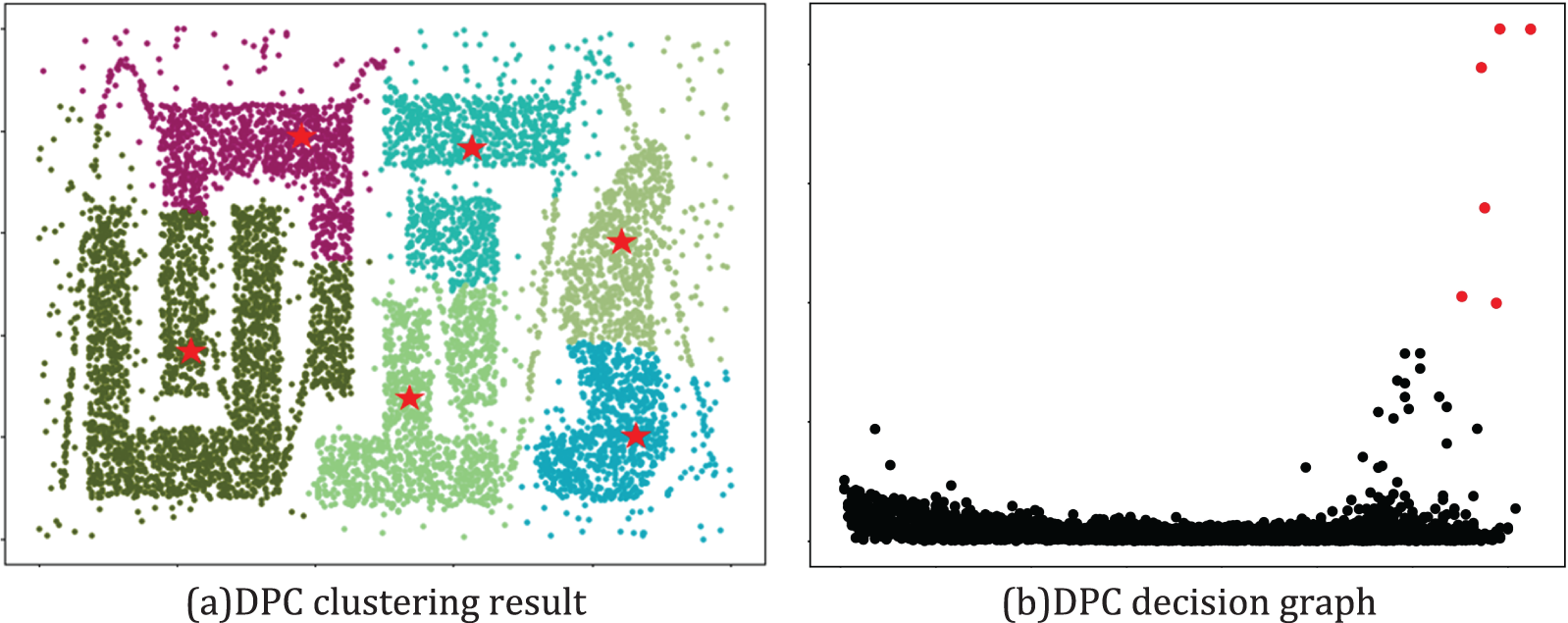
Figure 1: The decision graph and clustering results of DPC on the T4 dataset

(2) Once the cluster centers have been identified, the assignment strategy for other data points in the DPC clustering algorithm is relatively straightforward. The DPC algorithm assigns these data points to clusters that are denser than them. However, this assignment strategy fails to fully consider the impact of complex data environments. As shown in Fig. 1, when the DPC algorithm is applied to complex-shaped datasets, even if the cluster centers have been correctly selected, this assignment strategy can still lead to incorrect results.

2.3 Domain-Adaptive Density

To overcome the issue of suboptimal clustering results for data with vary density distributions (VDD), balanced distributions, and multiple-domain density maxima in DPC algorithms. Chen et al. [29] proposed a novel enhanced density clustering algorithm called Domain-Adaptive Density Clustering in 2021.

In the article, to overcome the problem of cluster loss in sparsity in VDD data for the DPC algorithm, a domain-adaptive density estimation technique known as KNN density is introduced. This method is utilized to identify density peaks in various density regions. By leveraging these density peaks, we can effectively identify the clustering centers in both dense and sparse regions, thereby effectively addressing the issue of sparse cluster loss. Assuming X is a collection of sample points in a d-dimensional space. To improve the algorithm’s performance on datasets with uneven density distributions and complex structures, we adopt KNN density to calculate the density of each sample point. The KNN density for any sample point i (where i ∈ X) is defined as shown in Eq. (6):

KDenti=1KDisti=K∑j∈KNNidij(6)

Definition 1: KNN Set. The KNN set of a sample point i, denoted as KNNi, satisfies the following conditions: (1) |KNNi|=K; (2) KNNi∈X/{x}; (3) ∀y∈KNNi,z∈xKNNi+{x},dxy≤dxz.

Here, K denotes the count of nearest neighbors for sample point i, and KNNi represents the set of K nearest neighbors of sample point i. If the average distance between sample point i and its K nearest neighbors is larger, then the KNN density of sample point i is higher.

2.4 The KD-Tree Nearest Neighbor Search Algorithm

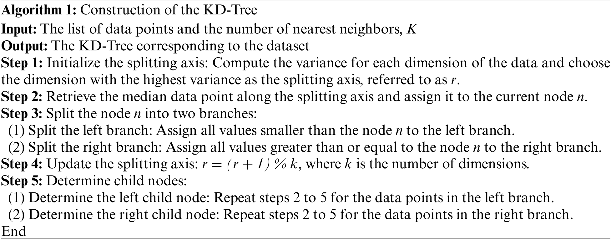
The KD-Tree [30], a spatial partitioning tree, is an effective data structure designed for efficient nearest neighbor search. Algorithm 1, to illustrate the construction process of the KD-Tree. It involves dividing the space based on the values of each dimension of the data points, thereby creating a multi-level binary tree structure. This facilitates the swift division of space into distinct regions, fostering convenience in searches and queries.

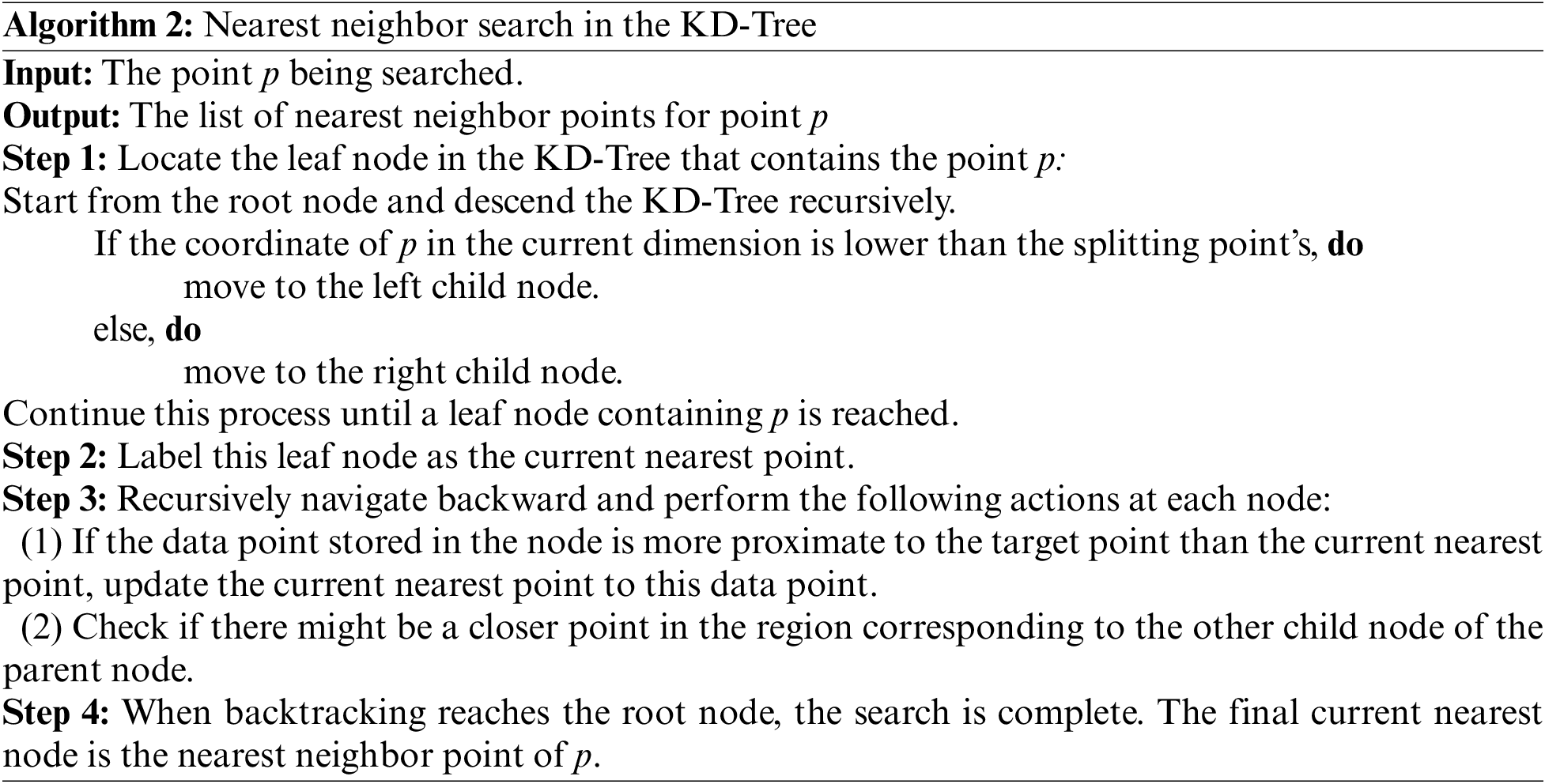
Algorithm 2 illustrates the nearest neighbor search process of the KD-Tree. It exhibits remarkable efficiency in handling substantial amounts of data.

In many clustering algorithms, a linear search is typically employed for neighbor search, which involves calculating the distance between each data point in the dataset and a reference data point in a sequential fashion. However, when dealing with large-scale datasets, this approach can become time-consuming and resource-intensive.

3  The Proposed Method

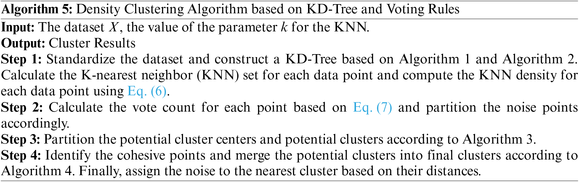
The algorithm can be categorized into four parts: (1) Constructing a KD-Tree; (2) Voting to select noise points and core points; (3) Identifying potential cluster centers; (4) Adhesive points identification and cluster merging.

3.1 Construct the KD-Tree

KNN has been proven to be an effective density estimation technique. However, for high-dimensional and large-scale datasets, the time complexity of obtaining the KNN set of a specific data point using traditional linear search methods exponentially grows with the size of the data. Therefore, this algorithm proposes the use of the KD-Tree nearest neighbor search method to obtain the KNN cluster of data points. The construction of the KD-Tree is outlined in Algorithm 1, and the nearest neighbor search process is described in Algorithm 2. Compared to the time complexity of O(N2) for linear search, the time complexity of using KD-Tree nearest neighbor search is O(NlogN).

Suppose we have a set of two-dimensional data points X = {A, B, C, D, E, F, G, H, I, J}. Firstly, we calculate the variance for each dimension of the data and select the x-axis as the splitting axis. Because point E is the median data point along the splitting axis, so KD-Tree is constructed by taking point E as the root node to partition the two-dimensional space, as shown in Fig. 2.

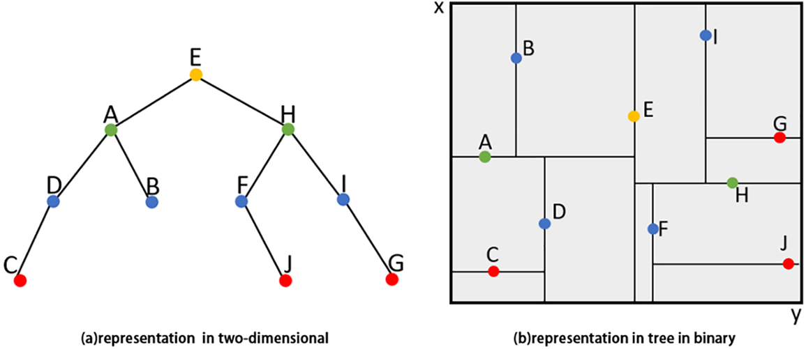
Figure 2: Example of constructing a KD-Tree for a two-dimensional dataset

3.2 Noise Point Identification

Definition 2: Mutual Nearest Neighbor (MNN), the KNN set of sample point i is denoted as KNNi, For any point j in KNNi, if it satisfies the condition: j∈KNNi∧i∈KNNj, then call point j as the MNN of point i, and the MNN set of sample point i is denoted as MNNi.

Just like shown in Fig. 3, The KNN set of point i and point j is depicted using arrows, it can be observed that point i is the KNN of point j, while simultaneously, point j is the KNN of point i, too. Thus, these two points are mutually designated as each other’s MNN.

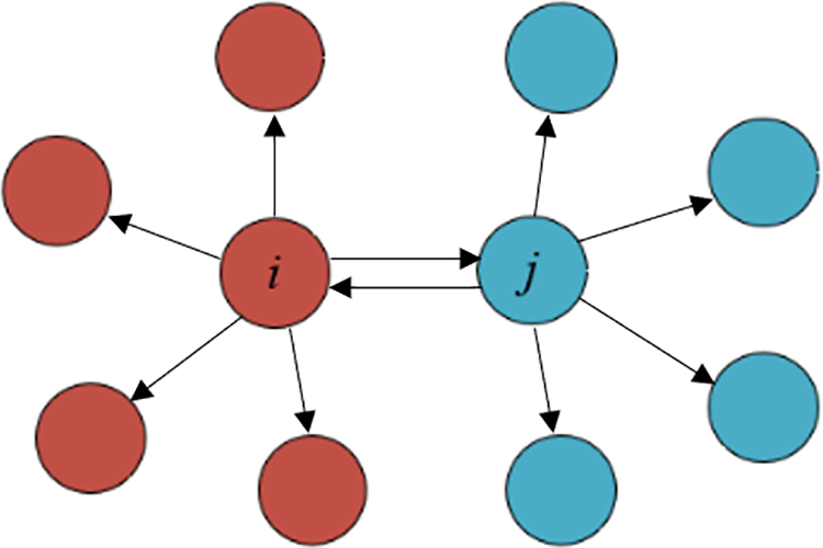
Figure 3: An illustration of the MNN among sample points

For the given point i (i ∈ X), the number of MNN for point i can be represented as |MNNi| the average number of MNN for each point in dataset X can be computed using Eq. (7).

|MNNAVG|=∑i∈X|MNNi||X|(7)

If |MNNi| meet the condition |MNNi| ≤ |MNNAVG|, then point i is classified as a noise. The purpose of this approach is to separate the low-density regions of the dataset into noises, thus preventing them from interfering with the final clustering results.

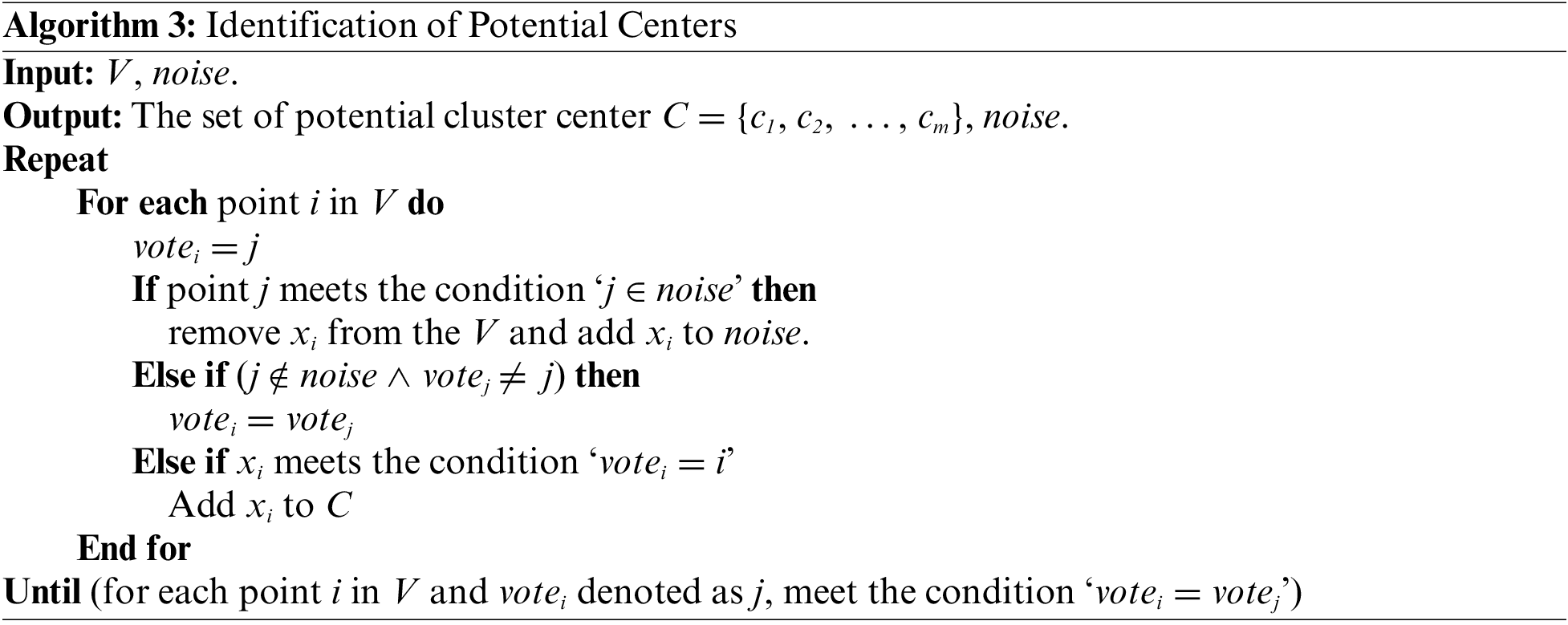
3.3 Potential Centers Identification

Definition 3: Voter, suppose X represents a set of data points in a d-dimensional space, where each point is considered a “Voter”. Each point casts one vote for the point in its KNN set with the highest KNN density. For any two points i and j (i, j ∈ X), if it satisfies votej = i, meaning point i is the KNN of point j with the highest KNN density, then point j is considered as a “voter” of point i. All the voters of point i are grouped as a potential cluster centered around point i.

Definition 4: Potential Cluster Centers, for a point z in the dataset X, if it satisfies votez = z, then point z is defined as a candidate cluster center. This means that point z is the point with the highest KNN density in its KNN set. We refer to these candidate cluster centers as potential cluster centers, as they represent the potential centroids of the underlying clusters.

As shown in Fig. 4, the yellow and blue samples represent two different clusters, while the black samples represent noise points. The arrows indicate the voting targets for each sample point. Points of the same color indicate that they belong to the same cluster. Among them, the two points represented by the pentagon and triangle are the centers of different clusters, denoted as x and y, respectively. It can be observed that votex = y and votey = y. Therefore, point y is a potential cluster center. At this stage, the clusters centered around point x should be assigned to the cluster where point y resides.

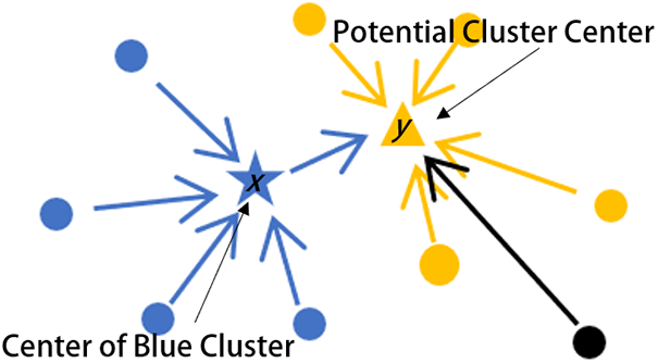
Figure 4: Identification of potential cluster centers

Let C = {c1, c2, …, cm} denote the number of potential centers, where m denotes the number of potential centers. Let V denote the set of samples obtained after removing the noise points from the dataset X. And the list of noise points is denoted as noise. The specific process for this stage can be shown in Algorithm 3.

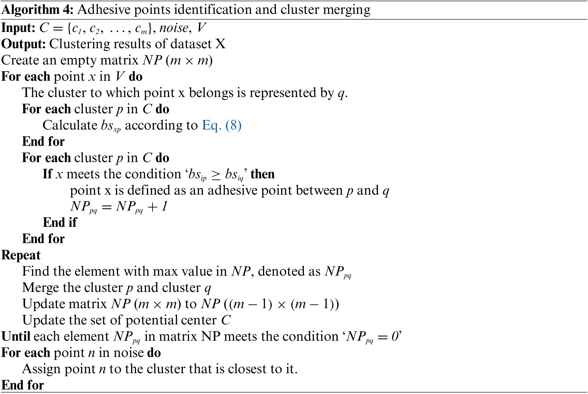
3.4 Adhesive Points Identification and Cluster Merging

To facilitate the amalgamation of clusters characterized by closely interconnected boundaries and similar densities, we propose the introduction of two novel concepts: the degree of cluster affiliation, denoted as bs, and the notion of cohesive points.

The degree of affiliation represents the extent to which a point belongs to its respective cluster. For any given point i (where i belongs to set X), let clusterp denote the cluster to which it belongs. The degree of affiliation, denoted as bsip, is defined for point i concerning clusterp as shown in Eq. (8).

bsip=∑j∈KNNiBj|KNN(xi)|,Bj={1,votej=p0,other(8)

Here, p represents the centroid of clusterp, which satisfies the condition that votep is equal to p.

Definition 5: Adhesive Points. Assuming we have two clusters, clusterp and clusterq, a point x belonging to either of these clusters is defined as a cohesive point if it complies with the following conditions. (1) x∈clusterp∪clusterq; (2) (x∈clusterq∧bsip≥bsiq)∨(x∈clusterp∧bsiq≥bsip).

Where bsim and bsin represent the degree of affiliation of point i to clusters m and n, respectively, a point i belonging to cluster m is identified as a cohesive point if its degree of affiliation bsin to the other cluster n is greater than or equal to bsim. If there exist adhesive points between two clusters, these two clusters will be merged into a single cluster. The specific merging strategy will be given in Algorithm 4.

Just as shown in Fig. 5 points p2, p3, p4, p5, p6, and p7 all belong to the K-nearest neighbor set of point p1. Cluster m is depicted in blue, while cluster n is depicted in red. Point p1 belongs to either cluster m or cluster n, and bsin = bsim. Hence p1 is classified as an adhesive point, depicted in yellow. This means that two clusters connected by an adhesive point are close neighbors and have similar local densities in that area, then we merge these two clusters. This process can help us quickly identify complex-shaped datasets.

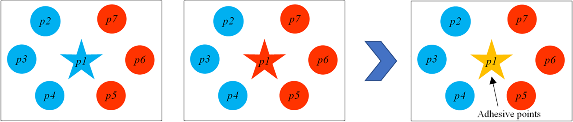
Figure 5: The process of identifying adhesive points

Let C = {c1, c2, …, cm} denote the set of potential centers. Let V denote the set of samples obtained after removing the noise points from the dataset X. The set of noise is denoted as noise, then the detailed process of this section is outlined in Algorithm 4.

3.5 Algorithm Description

Detailed steps of the density-based clustering algorithm based on KD-Tree and the voting rule are as follows:

Utilizing the Cth3 dataset as a demonstration, let us illustrate the clustering process of this algorithm. The Cth3 dataset consists of 1146 sample points, assuming there are 4 clusters in the correctly classified scenario. The procedure of the algorithm is outlined in Fig. 6 (with algorithm parameters ‘k’ = 28).

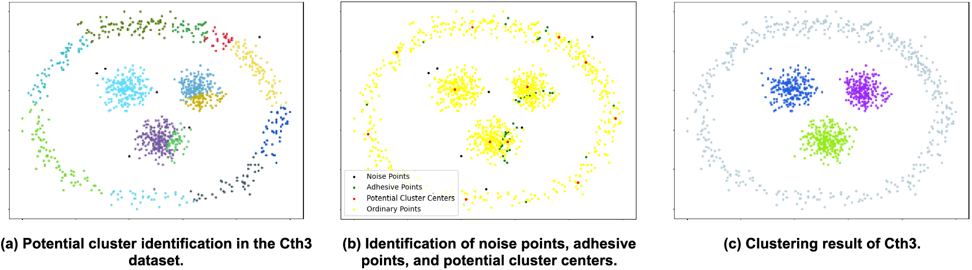
Figure 6: The clustering process of the Cth3 dataset

Just like shown in figures: Fig. 6a illustrates the results of identifying potential clusters after separating noise points and non-noise points. The black points represent noise points, while the colored clusters represent potential clusters. Fig. 6b displays the results after adhesive point identification. The black points represent noise points, the green points represent adhesive points, the yellow points represent non-noise points, and the red points represent potential cluster centers. Fig. 6c showcases the clustering results of the algorithm on the Cth3 dataset. It can be clearly seen that the algorithm accurately identifies the four clusters in the Cth3 dataset.

3.6 Time Complexity Analysis

The KDVR algorithm primarily consists of the construction and K-nearest neighbor search of the KD-Tree, identification of noise points and potential clusters, as well as the recognition of cohesive points and merging potential clusters. If the dataset contains n data points with d dimensions, the amount of nearest neighbors is set to k, and the count of potential cluster centers is denoted as c. The time complexity of the KD-Tree construction process is O(nlogn). The time complexity for identifying the K-nearest points to a certain data item by employing a KD-Tree is O(logn + k log k).

In the noise point identification process, each point casts a vote to the point with the maximum KNN density among its K-nearest neighbors, resulting in an O(n) time complexity. After the voting process, each data point is iterated to determine whether it is a noise point, resulting in a time complexity of O(n). In the potential cluster identification process, every data point is traversed, and in each iteration, it is checked whether the condition votevotei=votei is satisfied for point i, resulting in a time complexity of O(n). In the cohesive point recognition stage, each point’s K-nearest neighbors are traversed, and their cohesion to c clusters is computed, resulting in a time complexity of O(nkc). In the merging stage, the two clusters with the highest number of cohesive points are identified in a c × c matrix, and they are merged, requiring a time complexity of O(c2). Therefore, the time complexity of the KDVR algorithm can be summarized in Eq (9):

O(nlog⁡n)+O(log⁡n+klog⁡k)+3O(n)+O(nkc)+O(c2)=O(nlog⁡n+(n+kc+c2))(9)

It can be seen that the time complexity of this algorithm is largely influenced by the identification of cohesive points and the construction of the KD-Tree, which is O((n+1)logn)+O(nkc). Comparatively, the DPC and DBSCAN algorithms have the time complexity of O(n2), where c < k << n. When n is sufficiently large, this algorithm has a lower time complexity compared to both DPC and DBSCAN algorithms.

4  Experimental Results and Analysis

To confirm the efficiency of the KDVR algorithm, experiments were performed on 6 synthetic datasets [31,32] and 6 real-world datasets [33]. The results of the KDVR algorithm were compared with those of the following algorithms: DPC-KNN, DPC, DBSCAN, DPC-CM, and NNN-DPC algorithms. The experiment environment was a Windows 10 64-bit operating system, with an Intel(R) Core i5-8300H CPU and 8 GB of memory.

The implementation of the KDVR algorithm, DPC-KNN algorithm, DPC algorithm, DBSCAN algorithm, DPC-CM algorithm, and NNN-DPC algorithm was done using Python on the PyCharm 2019 platform. In the experiment, all datasets were preprocessed with min-max normalization. For the DPC-KNN algorithm, the number of clusters must be determined beforehand, and the parameter “dc” was chosen to achieve local optimal results. The values of “dc” were selected from {0.07, 0.14, 0.06, 0.11, 0.05, 0.03} for different datasets. Similarly, in the DPC algorithm, the parameter “dc” was chosen to achieve local optimal results, with values selected from {0.09, 0.15, 0.07, 0.13, 0.05, 0.04} for different datasets. For the DBSCAN algorithm, the parameters “ε” and “MinPts” were chosen to achieve local optimal results. The value of “ε” was selected from {0.16, 0.29, 0.08, 0.12, 0.13, 0.06}, and the value of “MinPts” was selected from {3, 5, 8, 4, 7, 12} for different datasets. In the KDVR algorithm, the parameters “k” and “p” were chosen to achieve local optimal results. The value of “k” was selected from {28, 20, 40, 50, 36, 60}. Measuring the advantage of a clustering algorithm using only one clustering metric is insufficient. Various clustering metrics can showcase various facets of clustering algorithms, enabling us to assess the proficiency of a clustering algorithm. Therefore, we adopted three metrics. These evaluation indicators include adjusted Rand index (ARI) [34], normalized mutual information (NMI) [35], and Accuracy (ACC).

ARI, or Adjusted Rand Index, measures the similarity between two clusters by considering different permutations of cluster labels. This metric is more accurate in reflecting the similarity between clustering results, and it also takes into account the measurement error caused by random probability, which increases the credibility of comparison results. The formula for calculating ARI is as follows:

AARI=RRI−E(RRI)maxRRI−E(RRI)(10)

where RRI represents RI, RRI = 2(TP + TN)/N(N-1), TP (True Positives) refers to the number of pairs that are both grouped into the same cluster and possess the same ground truth label, while TN (True Negatives) signifies the number of pairs that are assigned to different clusters but have the same ground truth label. The range of ARI is [−1, 1], with a value closer to 1 indicating a better clustering effect, while a negative value indicates that the labels are independently distributed, resulting in poor clustering performance.

NMI is the normalized version of MI, which measures the similarity between two clustering results to calculate the score. The formula for calculating NMI is as follows:

NNMI=−2×∑i=1n(S)∑j=1n(T)nijlb(N×nijni×nj)∑i=1n(S)nilb(niN)∑j=1n(T)njlb(njN)(11)

Here, n(S) and n(T) are the number of true clusters and the number of clusters obtained through clustering, respectively. nij is the number of samples that belong to cluster i in S and cluster j in T; ni is the number of samples within cluster i in S, and nj is the number of samples within cluster j in T. NMI measures the similarity between the true label set and the label set produced by clustering, with a range of [0,1]. A value closer to 1 indicates a more favorable clustering outcome.

ACC stands for clustering accuracy and is utilized to gauge the similarity between the clustering labels generated and the true labels provided by the data. The calculation formula is as follows:

ACC=∑i=1Nδ(si,ri)N,δ(x,y)={1,x=y0,x≠y(12)

where si and ri represent the clustering labels obtained for data xi and the true labels of data x respectively, and N stands for the total number of data points.

4.1 Results on Artificial Datasets

Comparison of the KDVR, DPC-KNN, DPC, DBSCAN, DPC-CM and NNN-DPC algorithm on 6 synthetic datasets with various characteristics. The selected synthetic datasets are presented in Table 1.

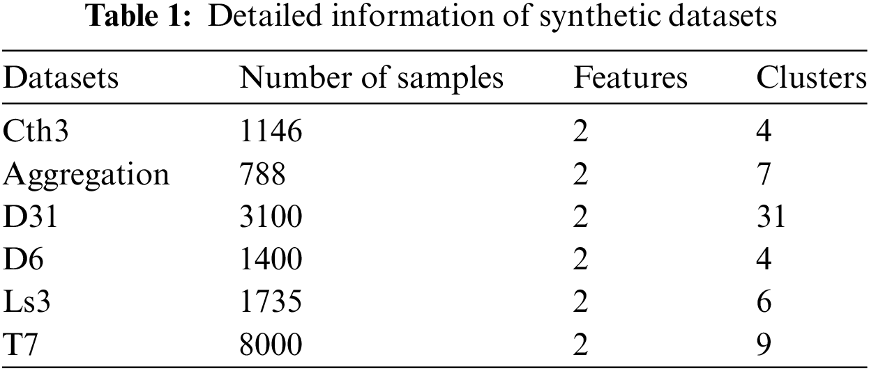
Fig. 7 visualizes the best clustering outcomes achieved by these algorithms on the aforementioned synthetic datasets mentioned above. The clustering outcomes of the DPC algorithm, as shown in (a), yield only acceptable clustering results on the Aggregation, D31, and D6 datasets. However, in the case of Cth3, the DPC algorithm erroneously allocates some points from the circular cluster to the central spherical cluster. It is evident that for complex-shaped clusters, such as Ls3 and T7, the DPC algorithm fails to achieve satisfactory clustering results. The clustering results of the DBSCAN algorithm, as shown in (b), DBSCAN can accurately identify clusters with complex shapes with fewer noisy points, such as Cth3, Aggregation, D6, and Ls3. However, for datasets with dense data points or excessive interference points, DBSCAN fails to produce good results. The clustering results of the DPC-KNN algorithm, as shown in (c), only achieve decent clustering results on the Aggregation and D6 datasets. In other clustering results, as a consequence of incorrect selection of initial cluster centers, erroneous clustering effects are observed. The clustering outcomes of the NNN-DPC algorithm, as shown in (d), achieve satisfactory clustering results on the Aggregation, D31, D6, and T7 datasets. However, it fails to effectively recognize the circular clusters situated externally to the spherical cluster in Cth3, as well as the clusters surrounding the spherical cluster in Ls3. The clustering results of the DPC-CM algorithm are displayed in (e), revealing that the algorithm performs well on spherical datasets and can effectively identify the spherical clusters in the shape-complex clusters. Compared to the DPC algorithm, it performs better on the D6 and T4 datasets. However, the algorithm still has certain limitations, identifying clusters with complex shapes on the periphery can be challenging. The clustering outcomes of the KDVR algorithm, as illustrated in (f), yield good clustering effects on all six datasets, this algorithm was able to accurately identify complex and dense clustering shapes. Although the performance on the Aggregation and D31 datasets was not the best.

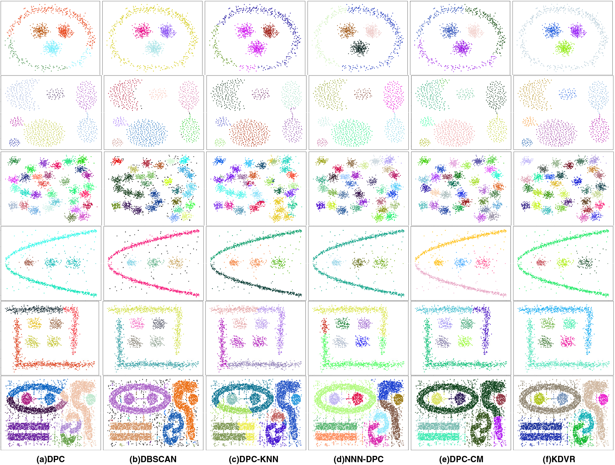
Figure 7: Clustering results on synthetic datasets

Table 2 presents the evaluation metrics of the KDVR, DBSCAN, DPC, DPC-KNN, DPC-CM, and NNN-DPC algorithms for clustering on the Cth3, Aggregation, R15, D31, D6, Ls3, and T7 datasets. Bold indicates the optimal clustering performance on each dataset.

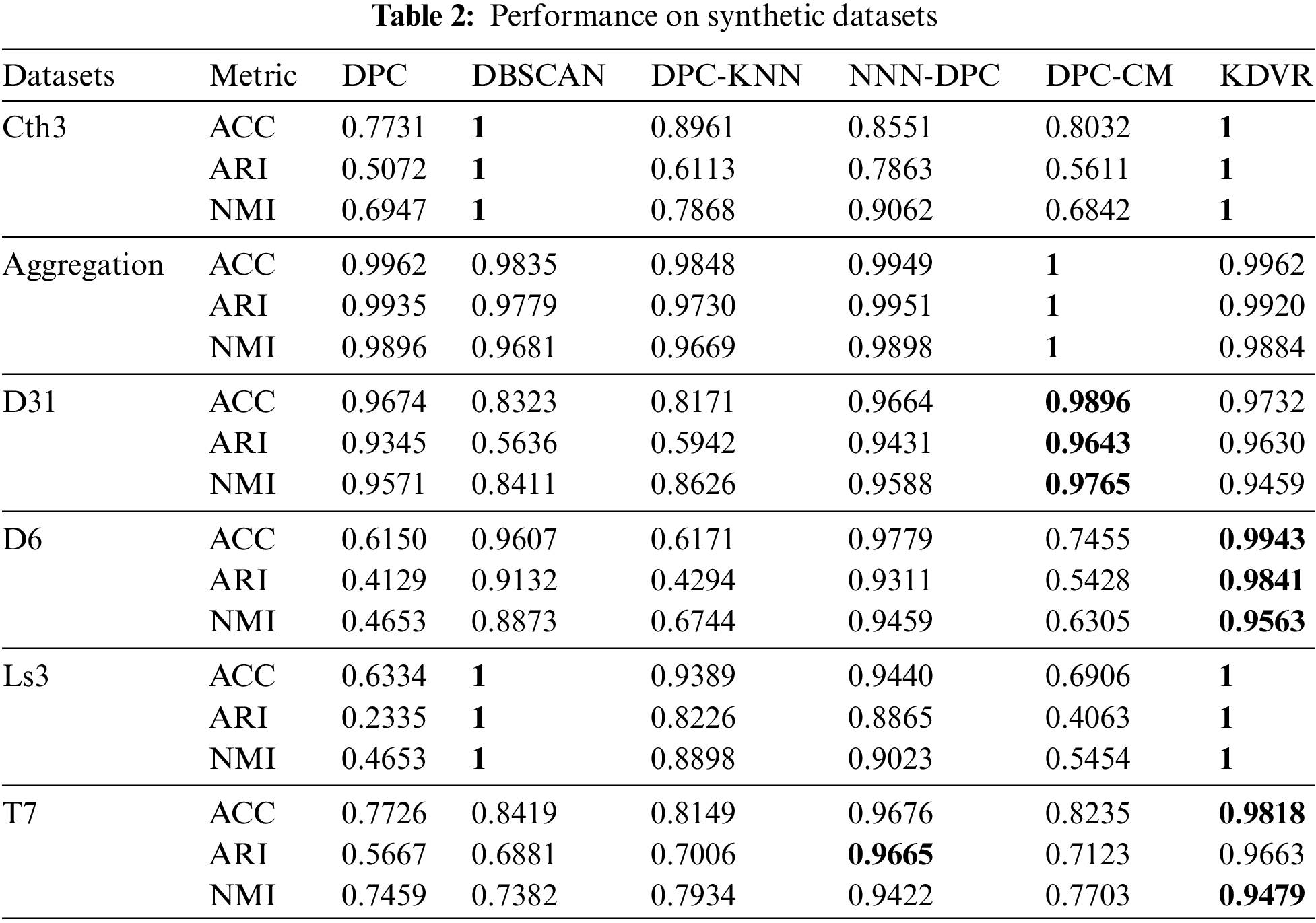
For complex shape data sets with multi-scale and cross-surrounding characteristics, the KDVR algorithm fully considers the impact of local density peaks on the clustering result, by improving the clustering center strategy, dividing the complex shape data set into multiple sub-clusters centered on the maximum points of local density. Then, the bonding point merges these sub-clusters to identify the clusters of complex shapes. Compared to other DPC improvement algorithms, the KDVR algorithm is more adept at handling such data sets. The experimental results on the cth3, D6, Ls3, and T7 data sets also confirm this. Although the clustering result of the KDVR algorithm is not optimal when processing data sets with uneven density, it is still close to the optimal level. This is because when the density variance is too significant, the decision result of the clustering center will be disturbed, leading to an inability to obtain the best clustering result. However, other algorithms cannot achieve good clustering results on both types of data sets simultaneously.

4.2 Result on UCI Datasets

To further contrast the clustering performance of the KDVR, DPC-KNN, DPC, DBSCAN, DPC-CM, and NNN-DPC algorithms on real-world datasets, ten diverse UCI datasets were selected for experimentation. These datasets vary in terms of their data size and dimensions, allowing for a better demonstration of the KDVR algorithm’s efficacy in handling high-dimensional data. Table 3 presents the information on these seven datasets.

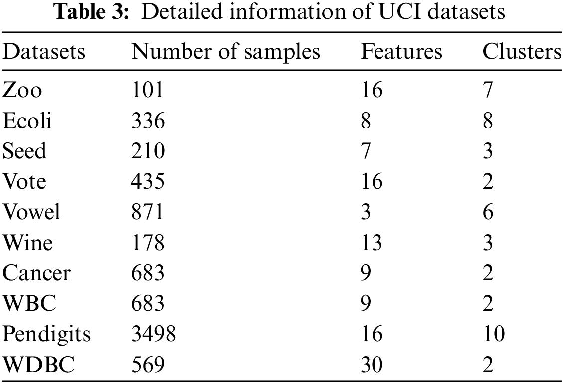
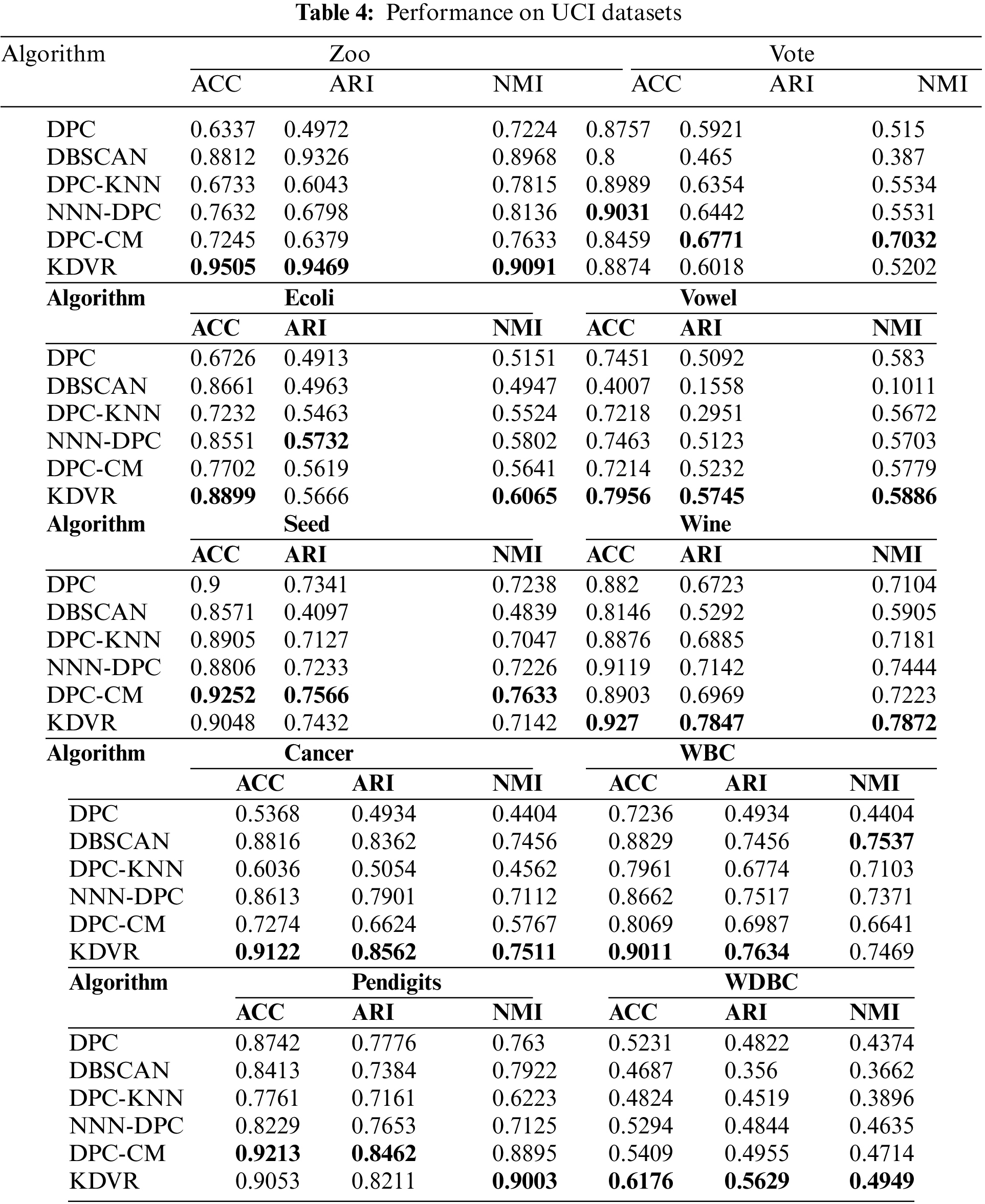
Table 4 showcases the evaluation metrics for clustering performed by the KDVR, DBSCAN, DPC, NNN-DPC, DPC-CM, and DPC-KNN algorithms on the UCI datasets. It can be observed that KDVR achieves better clustering results than the other algorithms on datasets such as Zoo, Vowel, Wine, Cancer, Pendigits, and WDBC. On the Ecoli, Seed, and WBC datasets, KDVR outperforms the other algorithms in terms of both evaluation metrics. While KDVR does not achieve the best results on the Vote dataset, it is very close to the optimal evaluation metric. Overall, KDVR demonstrates robustness and performance superiority over the other four algorithms in handling high-dimensional UCI datasets.

4.3 Parameter Sensitivity Experiment

The number of nearest neighbors, k, and the noise point control coefficient, p, are parameters that need to be controlled in KDVR. The value of k determines the size and shape of potential clusters, which in turn affects the number of clusters after merging. If the value of k is too large, points that do not belong to the potential cluster may be allocated to it. Conversely, if the value of k is too small, there will be an excessive number of potential clusters, which can impact the final merging of clusters. Typically, for dense datasets, a larger value of k is more appropriate, while for sparse datasets, a smaller value of k is preferable. The value of the noise point control coefficient, p, determines the number of data points classified as noise points in the dataset. It is important to choose an appropriate value based on the amount of noise present in the dataset.

Fig. 8 presents the impact of different values of k on three evaluation metrics in the T7 dataset. The optimal clustering results are achieved when the value of k is approximately within the range of (50, 85). This is because, within this range, the KDVR algorithm can accurately identify the correct number of clusters. Fig. 9 depicts the Running Time for various values of k on the T7 dataset. It can be observed that as the value of k increases, the algorithm’s running time gradually decreases. When 2 ≤ k ≤ 26, the algorithm’s running time reduction exhibits a significant gradient. Because the small value of k leads to identifying a substantial number of potential centers mistakenly, resulting in a higher time complexity. When 26 < k ≤ 74, the algorithm’s running time remains relatively stable. However, when k > 74, the gradient of the algorithm’s running time reduction starts to increase again. This is because, as k becomes sufficiently large, the algorithm tends to identify a considerable number of data points as a single potential cluster, resulting in a smaller number of potential clusters, which leads to erroneous clustering results.

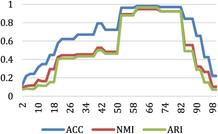
Figure 8: The values of evaluation metrics for various values of k on the T7 dataset

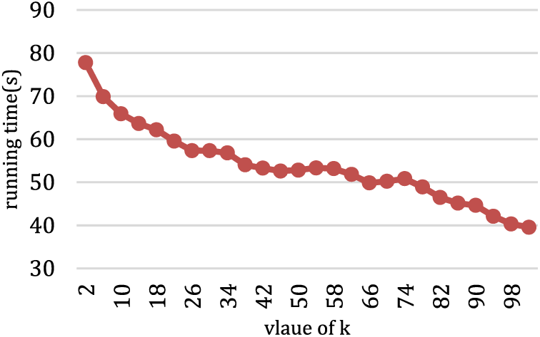
Figure 9: The running time for different values of k on the T7 dataset

5  Conclusion

This algorithm uses a KD-Tree to partition the entire dataset, and replaces the traditional density calculation method with the K-nearest neighbor density, thus avoiding the construction of similarity matrices and significantly reducing the computational cost. At the same time, the use of KNN density helps to identify clusters with uneven density. In addition, this algorithm introduces the concept of belonging degrees of sample points to each cluster and defines the concept of stickiness points between similar clusters on this basis. By using the concept of stickiness points, regions with similar densities are connected, merging potential clusters with high similarity, thereby effectively identifying clusters with complex morphologies and automatically determining the optimal number of clusters. Experiments have shown that this algorithm is not merely efficient but also possesses favorable clustering effects.

We noticed that the key to obtaining ideal clustering results in density-based clustering algorithms lies in correctly selecting the density clustering center. As long as there are enough data points in a region, the density-based clustering algorithm can recognize it as a cluster, which indicates that the cluster center must be the point with the densest concentration within its KNN, which is similar to the principle of voting election. This observation inspires us: to use a KD-Tree to partition the entire dataset, so that each data point can quickly find its KNN set, calculate the KNN density of each point, and then vote for the data point with the largest density among its KNN. In this way, we can find the point with the largest density in the local area, without having to calculate the similarity matrix, thereby improving the efficiency of the algorithm. At the same time, since the calculation of the KNN density only considers the distance of each point’s K-nearest neighbors, this facilitates the task of locating cluster center points within the local environment, rather than being affected by the density distribution of the entire dataset, making the algorithm able to identify sparse clusters in datasets with uneven density. In addition, through experiments, we also found that the K-nearest neighbors of points between dense and adjacent clusters have many points belong to other clusters, indicating that the density is similar and adjacent at the boundaries of the two clusters. Therefore, we merge such two clusters, ultimately enabling the algorithm to identify those clusters with complex shapes.

Although this algorithm improves efficiency to some extent, this mainly depends on the selection of an appropriate K value. If the K is too large, it may cause the entire dataset to be categorized into one cluster; if the K is too small, it may produce too many clusters, far from the actual number of clusters. So far, there is no clear conclusion about how to select an appropriate K value in experiments. In future experiments, we plan to optimize the K value selection strategy using decision trees. In summary, treating density clustering with KD-Tree and voting rules is an effective method. However, there are still some issues that need to be solved urgently, such as the K value selection strategy and how to more effectively judge the similarity between two clusters during cluster merging.

Acknowledgement: The authors of this article would like to thank all the members involved in this experiment, especially Mr. Hu, Mr. Ma, Mr. Liu, and Professor Wang, who contributed valuable insights and provided useful references and suggestions for the subsequent review of the experiment.

Funding Statement: This work was supported by National Natural Science Foundation of China Nos. 61962054 and 62372353.

Author Contributions: The authors confirm contribution to the paper as follows: study conception and design: Hui Du, Zhiyuan Hu; data collection: Zhiyuan Hu; analysis and interpretation of results: Hui Du, Zhiyuan Hu. Depeng Lu; draft manuscript preparation: Zhiyuan Hu. Depeng Lu. All authors reviewed the results and approved the final version of the manuscript.

Availability of Data and Materials: All the artificial datasets used in this article are sourced from: https://cs.uef.fi/sipu/datasets [34] and “K-means properties on six clustering benchmark datasets.” [35]; all the UCI Datasets used in this article are available from: https://archive.ics.uci.edu/ml.

Conflicts of Interest: The authors declare that they have no conflicts of interest to report regarding the present study.

References

1. M. G. H. Omran, A. P. Engelbrecht, and A. Salman, “An overview of clustering methods,” Intell. Data Anal., vol. 11, no. 6, pp. 583–605, 2007. doi: 10.3233/IDA-2007-11602. [Google Scholar] [CrossRef]

2. A. Dogan and D. Birant, “Machine learning and data mining in manufacturing,” Expert. Syst. Appl., vol. 166, pp. 114060, 2021. doi: 10.1016/j.eswa.2020.114060. [Google Scholar] [CrossRef]

3. J. Maia et al., “Evolving clustering algorithm based on mixture of typicalities for stream data mining,” Future Gener. Comp. Syst., vol. 106, pp. 672–684, 2020. doi: 10.1016/j.future.2020.01.017. [Google Scholar] [CrossRef]

4. Q. Zhang, C. Zhu, L. T. Yang, Z. Chen, L. Zhao and P. Li, “An incremental CFS algorithm for clustering large data in industrial internet of things,” IEEE Trans. Ind. Inform., vol. 13, no. 3, pp. 1193–1201, 2017. doi: 10.1109/TII.9424. [Google Scholar] [CrossRef]

5. A. Fahad et al., “A survey of clustering algorithms for big data: Taxonomy and empirical analysis,” IEEE Trans. Emerg. Topics Comput., vol. 2, no. 3, pp. 267–279, 2014. doi: 10.1109/TETC.2014.2330519. [Google Scholar] [CrossRef]

6. F. Hoppner, “Fuzzy cluster analysis: Methods for classification,” in Data Analysis and Image Recognition. USA: John Wiley, 1999. [Google Scholar]

7. P. Berkhin, A Survey of Clustering Data Mining Techniques, Grouping Multidimensional Data: Recent Advances in Clustering. Berlin, Heidelberg: Springer Berlin Heidelberg, pp. 25–71, 2006. [Google Scholar]

8. F. Cai, N. A. Le-Khac, and T. Kechadi, “Clustering approaches for financial data analysis: A survey,” ArXiv preprint ArXiv: 1609.08520, 2016. [Google Scholar]

9. D. Greene, A. Tsymbal, N. Bolshakova, and P. Cunningham, “Ensemble clustering in medical diagnostics,” in Proc. IEEE Symp. on Computer-Based Medical Systems, 2004, pp. 576–581. [Google Scholar]

10. M. Zaman and A. Hassan, “Improved statistical features-based control chart patterns recognition using ANFIS with fuzzy clustering,” Neural Comput. Appl., vol. 31, no. 10, pp. 5935–5949, 2019. doi: 10.1007/s00521-018-3388-2. [Google Scholar] [CrossRef]

11. J. Guan, S. Li, X. He, and J. Chen, “Peak-graph-based fast density peak clustering for image segmentation,” IEEE Signal Process Lett., vol. 28, pp. 897–901, 2021. doi: 10.1109/LSP.2021.3072794. [Google Scholar] [CrossRef]

12. F. Fang, L. Qiu, and S. Yuan, “Adaptive core fusion-based density peak clustering for complex data with arbitrary shapes and densities,” Pattern Recog., vol. 107, pp. 107452, 2020. doi: 10.1016/j.patcog.2020.107452. [Google Scholar] [CrossRef]

13. A. K. Jain, M. N. Murty, and P. J. Flynn, “Data clustering: A review,” ACM Comput. Surveys (CSUR), vol. 31, no. 3, pp. 264–323, 1999. doi: 10.1145/331499.331504. [Google Scholar] [CrossRef]

14. L. Kaufman and P. J. Rousseeuw, “Divisive analysis (program diana),” in Finding Groups in Data, 2008, pp. 253–279. [Google Scholar]

15. J. MacQueen, “Some methods for classification and analysis of multivariate observations,” in Proc. fifth Berkeley Symp. Math. Stat. Probab., 1967, vol. 1, no. 14, pp. 281–297. [Google Scholar]

16. Z. T. Birch, “An efficient data clustering method for very large databases,” in Proc. 1996 ACM SIGMOD Int. Conf. on Management of Data (SIGMOD’96), 1996, pp. 103–114. [Google Scholar]

17. S. Guha, R. Rastogi, and K. Shim, “Cure: An efficient clustering algorithm for large databases,” Inf. Syst., vol. 26, no. 1, pp. 35–58, 2001. doi: 10.1016/S0306-4379(01)00008-4. [Google Scholar] [CrossRef]

18. A. E. Ezugwu et al., “A comprehensive survey of clustering algorithms: State-of-the-art machine learning applications, taxonomy, challenges, and future research prospects,” Eng. Appl. Artif. Intell., vol. 110, pp. 104743, 2022. doi: 10.1016/j.engappai.2022.104743. [Google Scholar] [CrossRef]

19. M. Ester, H. P. Kriegel, J. Sander, and X. Xu, “A density-based algorithm for discovering clusters in large spatial databases with noise,” in Proc. KDD, vol. 96, no. 34, pp. 226–231, 1996. [Google Scholar]

20. A. Rodriguez and A. Laio, “Clustering by fast search and find of density peaks,” Science, vol. 344, no. 6191, pp. 1492–1496, 2014. doi: 10.1126/science.1242072. [Google Scholar] [CrossRef]

21. J. Xie, H. Gao, W. Xie, X. Liu, and P. W. Grant, “Robust clustering by detecting density peaks and assigning points based on fuzzy weighted K-nearest neighbors,” Inf. Sci., vol. 354, pp. 19–40, 2016. doi: 10.1016/j.ins.2016.03.011. [Google Scholar] [CrossRef]

22. R. Liu, H. Wang, and X. Yu, “Shared-nearest-neighbor-based clustering by fast search and find of density peaks,” Inf. Sci., vol. 450, pp. 200–226, 2018. doi: 10.1016/j.ins.2018.03.031. [Google Scholar] [CrossRef]

23. D. Yu, G. Liu, M. Guo, X. Liu, and S. Yao, “Density peaks clustering based on weighted local density sequence and nearest neighbor assignment,” IEEE Access, vol. 7, pp. 34301–34317, 2019. doi: 10.1109/Access.6287639. [Google Scholar] [CrossRef]

24. J. Jiang, Y. Chen, X. Meng, L. Wang, and K. Li, “A novel density peaks clustering algorithm based on k nearest neighbors for improving assignment process,” Phys. A Stat. Mech. Appl., vol. 523, pp. 702–713, 2019. doi: 10.1016/j.physa.2019.03.012. [Google Scholar] [CrossRef]

25. Y. H. Liu, Z. M. Ma, and F. Yu, “Adaptive density peak clustering based on K-nearest neighbors with aggregating strategy,” Knowl. Based Syst., vol. 133, pp. 208–220, 2017. doi: 10.1016/j.knosys.2017.07.010. [Google Scholar] [CrossRef]

26. Z. Yao, T. Fan, X. Li, and J. Zhao, “Density peaks clustering algorithm based on natural nearest neighbours and its application in network advertising recognition,” Int. J. Wireless Mobile Comput., vol. 18, no. 3, pp. 266–276, 2020. doi: 10.1504/IJWMC.2020.106775. [Google Scholar] [CrossRef]

27. Y. Shi and L. Bai, “Density peaks clustering based on candidate center and multi assignment policies,” IEEE Access, vol. 11, pp. 57158–57173, 2023. doi: 10.1109/ACCESS.2023.3283561. [Google Scholar] [CrossRef]

28. B. Liang, J. H. Cai, and H. F. Yang, “Grid-DPC: Improved density peaks clustering based on spatial grid walk,” Appl. Intell., vol. 53, no. 3, pp. 3221–3239, 2023. doi: 10.1007/s10489-022-03705-y. [Google Scholar] [CrossRef]

29. J. Chen and S. Y. Philip, “A domain adaptive density clustering algorithm for data with varying density distribution,” IEEE Trans. Knowl. Data Eng., vol. 33, no. 6, pp. 2310–2321, 2019. [Google Scholar]

30. J. L. Bentley, “Multidimensional binary search trees used for associative searching,” Commun. ACM, vol. 18, no. 9, pp. 509–517, 1975. doi: 10.1145/361002.361007. [Google Scholar] [CrossRef]

31. P. Fränti, “Clustering datasets,” Accessed: Dec. 27, 2023, 2017. [Online]. Available: https://cs.uef.fi/sipu/datasets [Google Scholar]

32. P. Fränti and S. Sieranoja, “K-means properties on six clustering benchmark datasets,” Appl. Intell., vol. 48, pp. 4743–4759, 2018. doi: 10.1007/s10489-018-1238-7. [Google Scholar] [CrossRef]

33. D. Dua and C. Graff, “UCI machine learning repository,” Accessed: Dec. 27, 2023, 2017. [Online]. Available: https://archive.ics.uci.edu/ml [Google Scholar]

34. N. X. Vinh, J. Epps, and J. Bailey, “Information theoretic measures for clusterings comparison: Is a correction for chance necessary?,” in Proc. 26th Annu. Int. Conf. on Machine Learning, 2009, pp. 1073–1080. [Google Scholar]

35. E. B. Fowlkes and C. L. Mallows, “A method for comparing two hierarchical clusterings,” J. Am. Stat. Assoc., vol. 78, no. 383, pp. 553–569, 1983. doi: 10.1080/01621459.1983.10478008. [Google Scholar] [CrossRef]