Time and Space Efficient Multi-Model Convolution Vision Transformer for Tomato Disease Detection from Leaf Images with Varied Backgrounds

1  Introduction

According to data collected from the Food and Agriculture Organization Corporate Statistical Database, the world produced 189.1 million metric tonnes of tomatoes on 5,167,087 hectares in 2021 [1]. Average production is reported as 36.6 metric tonnes/hectare (mT/ha) [2]. As per data revealed by Business Standard News, a decline of approximately 4% was observed from 2019 to 2022 in the production of tomatoes [3,4].

Being a rich source of iron, potassium, antioxidant lycopene, and vitamins A, C and K, tomatoes are useful in preventing cancer, maintaining blood pressure, regulating blood glucose levels, and heart health. Thus, the consumption of tomatoes reached approximately 234.5 million metric tons in the year 2023. As for the statistics, 80% of tomatoes are consumed fresh and 20% are consumed as purees, soups, tomato ketchup, pickles, juices, sauces, etc. [5]. Moreover, an increase of 3.3% in demand for tomatoes is estimated from 2024 to 2032 [6].

Thus, a decline in production and an increase in demand become a driving force to investigate the causes of tomato crop loss and minimize the loss. Based on the literature, disease-prone nature, climate change, decrease in soil fertility, and lack of water availability are the major causes of tomato crop loss [7]. The susceptibility of tomato crops to diseases such as early blight, late blight, gray leaf mold, etc., is one of the leading factors for its crop loss. In the past decade, the maximum crop loss was observed due to the viral disease ‘yellow leaf curl’ and the fungal disease ‘late blight’ [8,9].

Diseases in tomato crops can be marked in the form of lesions on leaves, stems, blooms, and fruits of plants. The unique visual symptoms of each disease can be used for its detection [10]. Manual disease detection relies on global features such as texture, shape, the color of disease spotsx, etc. [11]. These methods are time-consuming and require expertise in disease identification [12]. Also, these techniques fail to predict crop loss based on disease severity. In recent years, some researchers have applied Deep Learning (DL) models to accurately detect diseases using the datasets collected from laboratories or fields [13–16]. The DL models proposed by [7–12] gave the highest accuracy of 99.35% in disease detection if the training and testing datasets were part of the same dataset. The models proposed by Mohanty et al. [14] and Ferentinos [15] reported a training accuracy of more than 99% but the performance was reduced to 35% when tested on an unseen dataset [13]. Now, Barbedo [16] highlighted asome factors influencing the performance of DL models applied to detect plant leaf diseases. They claimed that the proposed approaches still lack developing a generic tool for assisting farmers in real life.

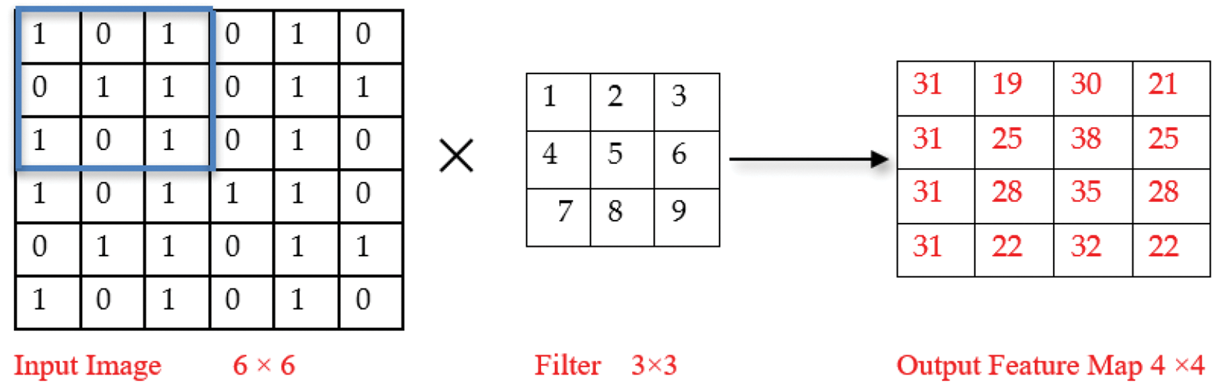
Further advancements in DL techniques and the success of transformer neural networks in Natural Language Processing (NLP) tasks inspired the researchers to extend their applicability in image classification. Thus, the authors in [17] introduced Vision Transformers (ViT) for plant disease detection. The model exhibits slightly lower recognition accuracy than similar sized Convolutional Neural Networks (CNNs) trained on the same datasets. This decrease in accuracy can be attributed to two main reasons. Firstly, transformers process images as patches, leading to the omission of important local features like edges and lines, resulting in a loss of fine-grained details that CNNs captures well. Secondly, the attention layer in transformers may not be as efficient as the convolutional layers in CNNs for extracting fine details in terms of local features. To improve the performance of ViT model, Wu et al. proposed a hybrid model that incorporates a convolutional layer within the transformer architecture and introduced convolution to the ViT model. They proposed a Convolutional vision Transformer (CvT) model [18]. In a CNN, the convolution is performed on the input data using a filter to produce a feature map [19]. We perform element-wise multiplication of the input matrix and the filter element followed by calculating sum of the results to extract a feature. For example, Input matrix: [101011101], and filter: [123456789] are used to calculate the convolved feature as demonstrated below. The numbers in the input matrix and the filter that are multiplied together are represented with the same color.

Convolved Feature=(1×1)+(0×2)+(1×3)+(0×4)+(1×5)+(1×6)+(1×7)+(0×8)+(1×9)(1×1)+(0×2)

Similarly, all other values of the feature map are calculated as shown in the output feature map below.

Convolution operation in the VGG16 model applies filters to extract hierarchical features, emphasizing spatial patterns. In VIT and CvT models, convolution is replaced by self-attention mechanisms, enabling global contextual understanding, and facilitating improved recognition of intricate disease-related details.

However, Deep learning (DL) and computer vision techniques have proven their potential in the automation of disease detection in tomato crops. Noisy background, identification of multiple diseases on the same plant or part of the plant, and varying symptoms of the same disease in different geographical regions create difficulty in disease identification [20]. Moreover, high computation costs, long training time, and the requirement of large storage space to deploy a DL model restrict their real-life implementation using handheld devices such as mobile phones, drones and IoT devices. Moreover, the size and quality of the dataset used for training the DL model highly affect its performance in disease detection [21]. This leaves room for improvement in existing models.

To address the above-mentioned challenges, we propose a tailored multi-model architecture ‘Swift-Lite-CvT’ for disease detection in tomato plants to assist farmers and plant pathologists. The architecture is an integration of customized VGG16, ViT, and CvT models.

The key contributions of this study are listed below:

•   Preparing the labelled dataset including 13 tomato disease classes with plain, as well as, complex backgrounds.

•   Developing a multimodal ‘Swift-Lite-CvT’ deep learning-based architecture for tomato disease detection.

•   Improving disease detection accuracy for datasets with complex backgrounds and multiple diseases on the same plant.

•   Reducing computation time and increasing the reliability of the DL-based architectures applied for tomato disease detection.

The remaining structure of the paper is as follows: Section 2 provides an overview of the related works. Section 3 presents the materials and methods including details about dataset preparation, and models employed for the experiment. Section 4 focuses on the experiments, Section 5 demonstrates the results obtained from trained models. Section 6 illustrates the discussion and provides a comprehensive analysis of the findings. The last section highlights the conclusions drawn and the future scope.

2  Related Works

In this section, we present the applied models, and the advantages and limitations observed in works available in literature. Thangaraj et al. [22] reviewed the challenges and limitations of the ML andDL models employed for tomato plant disease identification. Agarwal et al. [23] introduced a CNN model and evaluated its performance against established CNN models like VGG16, MobileNet, and InceptionV3. The proposed model achieved an accuracy of 91.20%, surpassing all the above-mentioned models. Similarly, Ahmad et al. [24] collected a real field dataset comprising 317 images and applied augmentation techniques to increase the dataset size. Finally, they prepared an augmented dataset comprising 15,216 images. They applied VGG-16, VGG-19, ResNet, and Inception V3 models on the collected as well as augmented datasets. Inception V3 achieved the highest accuracy of 99.60%, and 93.70% on the augmented and collected dataset, respectively. Norria et al. [25] proposed an automated system for tomato diseases classification using ResNet50 CNN model. This system classifies the tomato leaf dataset into healthy, septoria leaf and late blight classes. The system reported an average accuracy of 92.08%. Next, Chowdhury et al. [26] used a plant village dataset for their studies. They applied ResNet18, MobilenetV2, InceptionV3, and DenseNet201 for binary classification, 6-class classification and 10-class classification. InceptionV3 outperformed and achieved an accuracy of 99.2% for binary classification. The DenseNet201 model attained 97.99% and 98.05% accuracy for 6-class and 10-class classification, respectively. This study has the potential for the early identification and automated diagnosis of diseases in tomato crops. Furthermore, by integrating a feedback system, this framework can offer valuable insights, treatments, preventive strategies, and disease control techniques, ultimately resulting in enhanced crop yields. In line with the previous works, Gonzalez-Huitron et al. [27] developed a GUI interface for the detection of disease in tomato leaves. For the experiments, they implemented lightweight CNN architectures on Raspberry Pi 4 microcomputer. Hassan et al. [28] developed an efficient DL model for disease detection in tomato leaves. They compared four DL models namely InceptionV3, InceptionResNetV2, MobileNetV2 and Efficient-NetB0 on the plant village dataset. EfficientNetB0, and MobileNet attained 99.56%, and 97.02% accuracy, respectively. However, MobileNet reports lower accuracy than EfficientNetB0, but its smaller number of parameters and lightweight architecture promote its real-life application using mobile devices. The model fails to handle noisy dataset, and complex background. Thus, leaves a scope for further research.

In all the above-discussed research works, a large training dataset is required. To address this issue, the authors in [29] applied a hybrid model developed using a Conditional Generative Adversarial Network (C-GAN) and a DL model. The model can generate synthetic images similar to real images and increase the dataset size. The authors applied DenseNet121 model for 5-class, 7-class and 10-class classification on the generated dataset and reported accuracy of 99.51%, 98.56% and 97.11%, respectively. Zhou et al. [30] used AI challenger dataset for tomato leaf disease detection using restructured residual dense network (RDN). This approach reduces the number of parameters, so it is an efficient model with less computation and attained an accuracy of 95%. Now, Paymode et al. [31] focused on disease detection in grapes and tomato crops. They collected real field datasets from Nashik, and Maharashtra, India for grape crops and used publicly available plant village dataset for tomato crops. They applied VGG16 model and achieved an accuracy of 95.71% for disease classification in tomatoes and 98.40% for grapes. The study deals with challenges in both collecting and preparing a genuine dataset, as well as the limited number of epochs used for training the data. Consequently, deploying this model on handheld devices with limited storage could pose challenges.

Similarly, Vadivel et al. [32] also applied VGG16 CNN model and gained a high accuracy of 99.5% on the plant village dataset. This study faces a challenge when tested on real-life datasets. Similarly, Tarek et al. [33] evaluated several DL models like Alex Net, ResNet50, InceptionV3, MobileNetV1, MobileNetV2 and MobileNetV3 on plant village datasets for tomato disease detection. MobileNetV3 model outperformed all the above-mentioned models and attained an accuracy of 99.81%. Moreover, the size of the model is reduced to 34 MB. Wang et al. [34] observed that existing classifiers face issues in recognizing diseases with similar symptoms, more than one disease on the same plant, and small disease lesions. Therefore, they collected the dataset from the three districts of Beijing, China and applied a combination of CNN models and transformer architecture for tomato disease detection. The model reported an accuracy of 96.30% on the real dataset. The authors in [35] used four publicly available datasets namely plant village [36], ibean [37], AI challenger [38] and PlantDoc [39] for plant disease detection. They applied Inception convolutional vision transformer model on the above-mentioned datasets and achieved an accuracy of 99.97%, 99.22%, 86.89% and 77.54%, respectively. But the model reported a low accuracy of 77.54% when applied to dataset with a complex background. Now, Alzahrani et al. [40] compared the performance of DenseNet169, ResNet50V2 and ViT models on the publicly available dataset [13] comprising leaf images with a plain background. DenseNet121 achieved the highest accuracy of 99%. Also, the models are intense and cannot be implemented on handheld devices. And, the model fails to deal with real-world data. The most related works and their limitations are summarized in Table 1.

According to the above discussion, it is evident that the employed DL models are less efficient in disease prediction from the dataset with complex backgrounds. Moreover, the models proposed so far have higher computational and memory requirements [17]. Thus, there is a need for an architecture that can correctly detect disease from the plain as well as complex background. Simultaneously, it should be small so that it can be implemented on handheld devices to assist farmers in automatic crop monitoring and disease prediction. To meet these challenges, we propose a multimodal ‘Swift-Lite-CvT’ that correctly performs multi-class classification of the dataset comprising tomato leaf images with plain and complex backgrounds. The convolution operations performed by this model are efficient in capturing local spatial details, whereas its transformer part is effective in analyzing the global context of an image. Therefore, using the insights from the local and global features, the model can classify the image to the correct class irrespective of type of the background. Moreover, we focus on minimizing the computation and storage requirements of the model.

3  Materials and Methods

In this research, we applied various DL techniques to detect tomato leaf diseases and classify them into 10, 11 and 13 classes. For correct multi-class classification, we employed pre-trained networks, namely VGG16, Vision Transformer, and CvT models. Pretraining on large datasets of tomato leaves acts as an initialization, allowing the model to start with already optimized parameters. While pretraining, the model learns to recognize the shape, size, boundaries, etc. Further training of the pre-trained model on the labelled dataset and its fine tuning helps in faster converging, making the training process more computationally efficient. To further improve the reliability, and reduce the training time we designed a customized model “Swift-Lite-CvT”, based on CVT model [41,42]. The depth of transformer layer in the proposed model is reduced from 2 to 1 in second block, and 10 to 1 in the third block. Additionally, the number of attention heads are reduced from 3 to 2, and from 6 to 4 in the second and third blocks, respectively. These changes make the proposed model more lightweight and computationally efficient than the original CvT. The classification strategy followed in this study is illustrated in Fig. 1.

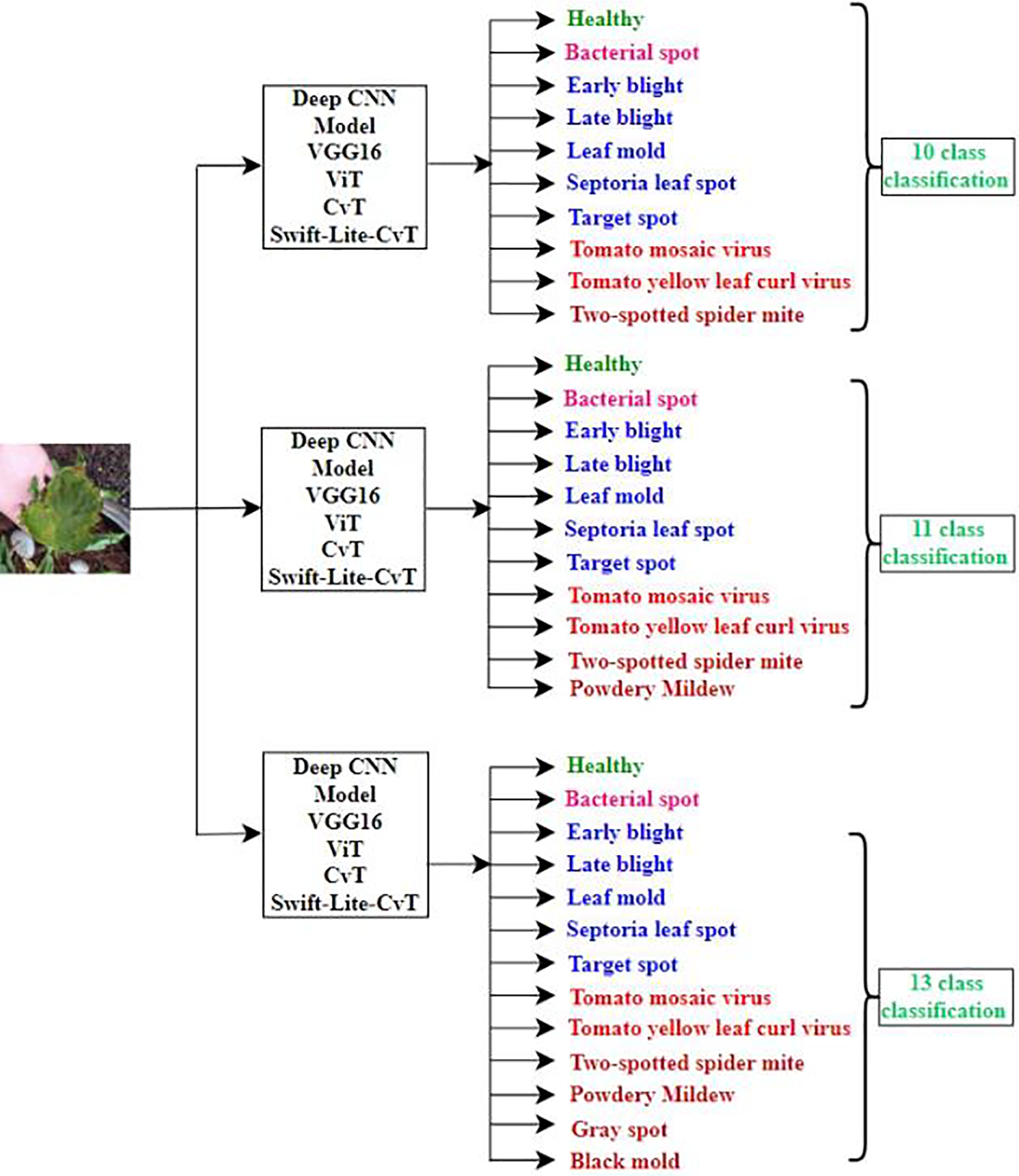
Figure 1: Classification strategy: Models implemented for multi class classification

3.1 Datasets

In this study, three distinct datasets were employed, namely Plant Village [43], Taiwan dataset [44], and PlantDoc dataset [45] comprising tomato leaves. The dataset comprises tomato leaf images with a plain grey background and complex background having rotten leaves, stones, soil, dry leaves, etc. The dataset with complex background is prepared to train the model for real-life datasets captured directly from fields. The dataset captured from fields cannot have a plain background, thus, to enable the model for classifying real-life images to the correct disease or healthy class, the dataset with a complex background is prepared.

3.1.1 Plant Village Dataset

The Plant village dataset [43] comprises 50,000 images of tomato leaves labelled with ten disease classes such as bacterial spot, early blight, healthy, late blight, leaf mold, septoria leaf spot, target spot, tomato mosaic virus, tomato yellow leaf curl virus and two-spotted spider mite. Each image contains a single leaf and a plain background. A plain background means that there is a clear demarcation between the leaf and the background region. The background region is uncoloured without any object. Sample images for this dataset are shown in Fig. 2. This dataset is divided into training and testing datasets in the ratio of 80:20, respectively.

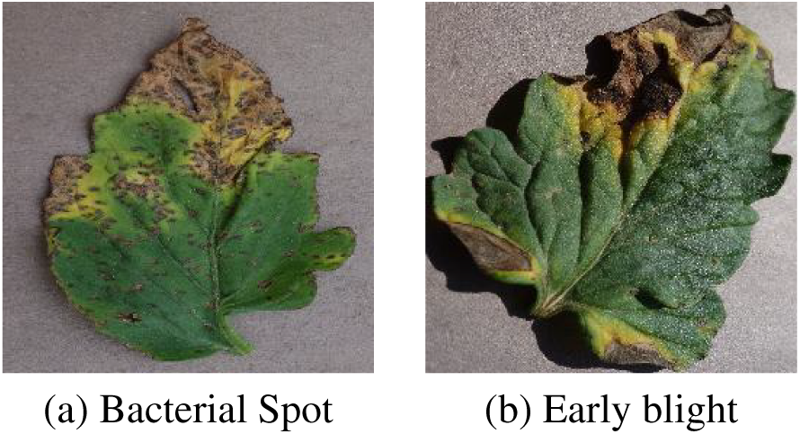
Figure 2: Sample images from plant village dataset with plain background [43]

3.1.2 Taiwan Dataset

The Taiwan dataset of tomato leaves [44] comprised images labelled with six categories such as bacterial spot, black leaf mold, gray leaf spot, healthy, late blight and powdery mildew. This dataset contains images with a single leaf, multiple leaves, a plain background and a complex background. A complex background contains one or more objects. Thus, there is no clear demarcation between the leaf and the background region. The sample images are shown in Fig. 3. The dataset comprises 622 original images. The size of images varies, so we unified them to 224 × 224. We also applied data augmentation techniques such as centre cropping, random cropping, horizontal flipping, etc., to increase the dataset size. The details of the dataset are shown in Table 2.

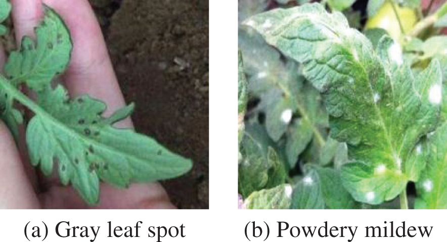
Figure 3: Sample images of Taiwan dataset of tomato leaves with complex background [44]

3.1.3 PlantDoc

The PlantDoc dataset [45] comprising 2,598 images was labelled with 13 plant species and 17 classes of diseased and healthy leaves. Also, the dataset contains human hands in the background as well as other plant parts forming the complex background. Sample images of this dataset are shown in Fig. 4.

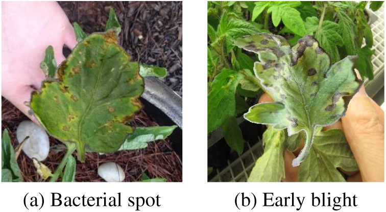
Figure 4: Sample images from PlantDoc dataset with complex background [45]

3.1.4 Customized Tomato Leaf Dataset (CTL Dataset)

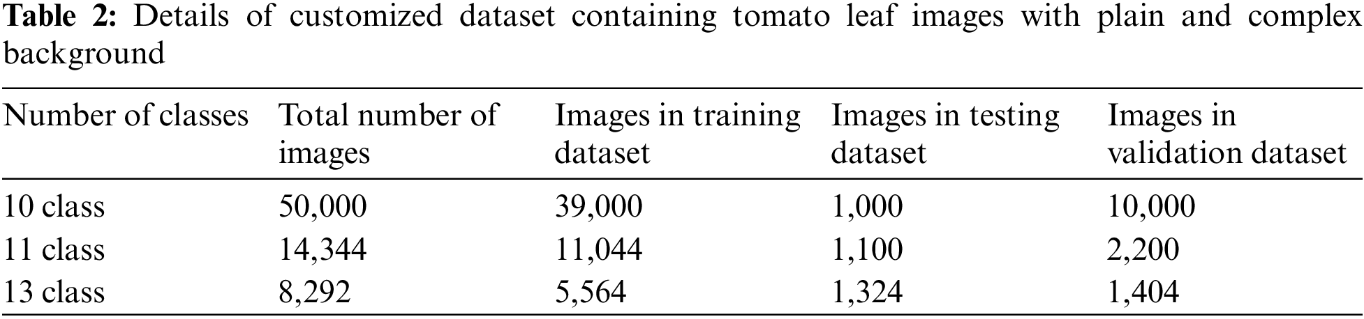
To extend the applicability of the designed DL model “Swift-Lite-CvT”, we collected images from all the three above-mentioned datasets. Using solely plain background images proved insufficient for achieving accurate detection and classification of tomato plant leaf diseases in real life. So, we included images with plain and complex backgrounds. This enables better training of the model on the versatile dataset and improves the robustness of the model. Here, robustness is the potential of the model to accurately classify tomato leaf images captured with plain as well as complex backgrounds. Thus, the performance of the model remains consistent in data collected in a laboratory or a field. Table 2 shows the number of classes, dataset size for training, testing and validation of the model.

3.2 DL Models

In this study, we have deployed the following four DL models, based on deep CNN and transformer architectures.

3.2.1 VGG16

VGG16 [46] model used for plant leaf disease detection. The filter sizes were reduced to 11 and 5 in the first and second convolutional layers, respectively. Also, the large-sized kernel filters were replaced with multiple 3 × 3 kernel sized filters. The modification enables the model to capture more localized features within the images. To enhance the performance and generalization of the VGG16 model, augmentation techniques such as rotation, scaling, and flipping, were applied to the input images. The variation caused by augmenting the training data helps to improve the robustness of the model. Hence, the model becomes more efficient in classifying various plant diseases. Our selection of VGG16 was influenced by its compact architecture with a reduced number of layers and parameters. Its proven reliability and high accuracy of 99.53%, 95.2% and 89% for tomato disease detection demonstrated in [11,47,48] respectively further supported our choice.

3.2.2 Vision Transformer (ViT)

The Vision Transformer (ViT) [49] has emerged as a prominent neural network architecture in the field of computer vision. In this model, the convolution neural network component is replaced with the transformer block which was earlier designed for handling sequential data. Thus, ViT adapted to handle images by dividing it into a sequence of patches. It considers each patch as a token of the sequence and learns to correctly classify images with plain or complex backgrounds.

In this architecture, initially, the input image is divided into patches of equal size, as depicted in Fig. 5. Each patch is then flattened into a 1-D array vector and subsequently embedded with positional encoding. This encoding step helps to capture the spatial information of each patch within the image. The encoded patches are passed through the transformer encoder block. This block consists of self-attention mechanisms and Multi-Layer Perceptron (MLP) heads, which enable the model to capture both local and global dependencies within the image. Finally, classification is performed using the transformer architecture, leveraging the learned representations from the encoded patches. The ViT architecture divides the input image into patches, encoding with positional information, and then processing them through transformer encoder blocks for accurate image classification. The potential of ViT in extracting local as well as global features from an image and maintaining spatial relationships within an image motivated us to employ this model for tomato disease classification.

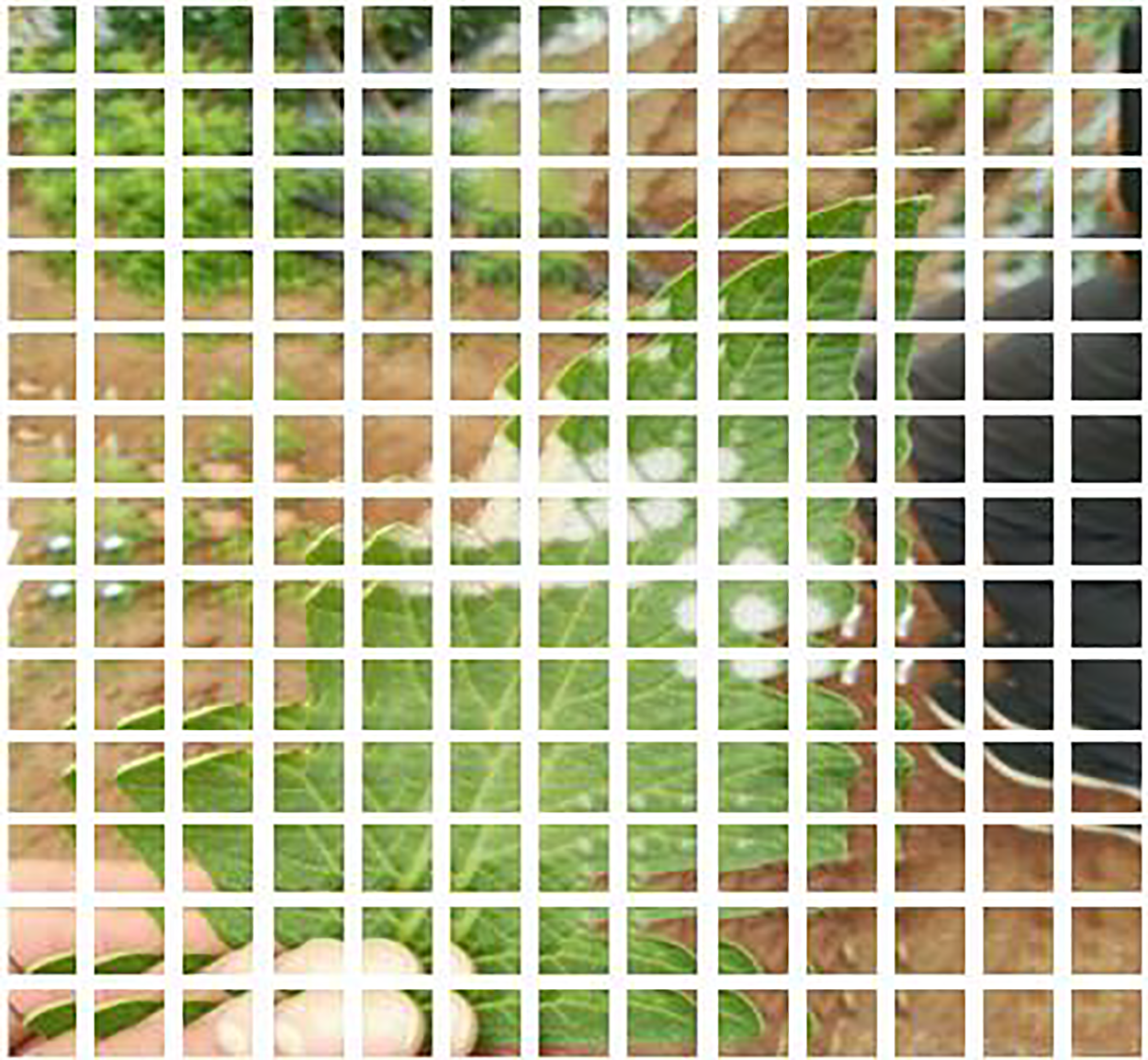
Figure 5: Input image in form of patches

3.2.3 Convolutional Vision Transformer (CvT)

The CvT [50] architecture represents an improved version of the Vision Transformer that enhances performance and efficiency by incorporating convolutions. It combines the advantages of both CNNs and transformers. It adopts a hierarchical, multi-stage architecture, enabling progressive feature extraction and refinement. Its basic architecture is shown in Fig. 6.

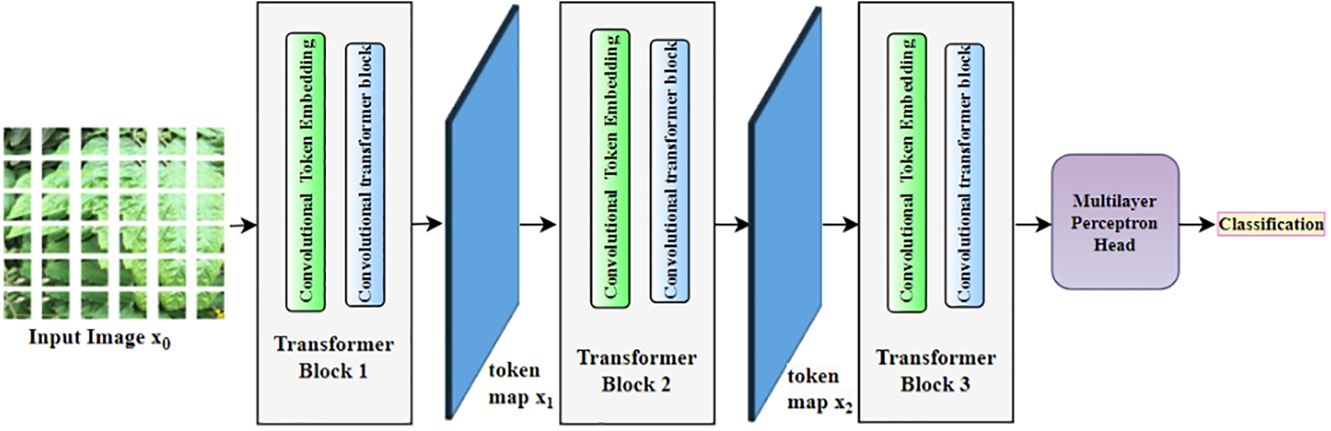
Figure 6: Convolution vision transformer model for tomato disease detection

CvT model initiates its task with tokenization, followed by transformation and classification. The steps followed are illustrated below: Initially, a convolutional layer is employed to transform the image’s local features into tokens, which are subsequently processed by the transformer block and normalized through layer normalization. Now, the transformer blocks capture extended-range dependencies and establish an interaction among tokens. These transformers incorporate multi-head attention. Each stage employs a unique number of heads. For example, number of heads are 1, 3, and 6 across three stages. This variation facilitates adaptable and dynamic receptive fields. Upon completion of processing through all stages, a classification token (cls token) is introduced at the outset, and the token representations are aggregated for the classification task. A MLP is then applied to this pooled representation for the final classification.

The experimental results presented in [14,27,50] validate that CvT outperforms both the Vision Transformer and ResNet model. Also, the removal of the positional encoding step, which is typically used in transformers to transform input images into patches reduces the training time of the model. Despite removing positional encoding, the CvT model maintains its performance. The CvT architecture leverages the advantages of convolutions to efficiently process input images while eliminating the need for explicit positional encoding. This motivated us to select CvT model for our research.

3.2.4 Modified Convolutional Vision Transfer (Swift-Lite-CvT)

We modified the architecture of the CvT model to improve its efficacy for tomato disease detection. The architecture of “Swift-Lite-CvT” is shown in Fig. 7. The modified version of CvT “Swift-Lite-CvT”, retains the hierarchical structure of the original CvT to preserve its proficiency in extracting local features. But the number of attention heads in the transformers is modified to 1, 2, and 4 across the three stages. Also, the depth of the transformer blocks is simplified and set 1 for all stages. Like the original CvT, after processing the tokens are pooled and subsequently channeled through a MLP for the classification task.

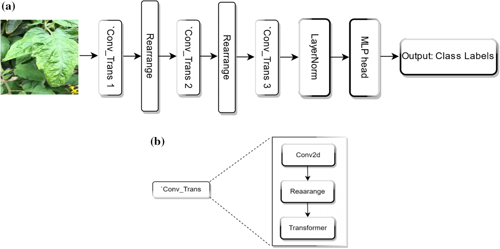
Figure 7: (a) Overall architecture of proposed Swift-Lite-CvT architecture. (b) Details of Conv_Trans block

4  Experiments

In this section, the details of the experimental setup, implementation details, and evaluation metrics employed are discussed.

4.1 Experimental Setup

For the experiments, a workstation with i9 processor, RTX 3070 GPU, 64 GB RAM and 3 TB hard disk is used. The pytorch and transformer architecture library are used for developing DL models implemented in this research.

4.2 Implementation

In the first block, ‘Conv_trans1’, convolutional token embedding is done with a 2D convolution, utilizing a kernel size of 7 and a stride of 4. The output channels generated by this convolution are referred to dim with a default value of 64. Now, the feature map obtained is transformed into tokens. These tokens are normalized through LayerNorm. Transformer block comprises a single transformer layer and the multi-head attention mechanism utilizes heads [0]. The token map generated is designated as ×1. In the second block, “Conv_trans2”, convolutional token embedding employs a 2D convolution with a kernel size of 3 and a stride of 2. The number of output channels is determined as a scaled-up version of the dim from the previous stage. This scaling factor depends on the ratio of the attention heads in this stage to the previous stage, specifically heads [1]/heads [0]. Similar to block 1, the convolution’s output is restructured into tokens and subsequently normalized. The transformer block contains a solitary transformer layer. In this layer, the multi head attention mechanism employs heads [1], which are configured to use two attention heads. It generates a token map denoted as ×2. Next, in the third block Conv_trans3, works similar to Conv_trans2 except the ratio of heads is calculated as [2]/heads [1], and its multi-head attention mechanism utilizes heads [2]. Also, the multi-head attention has been configured to employ attention heads [4] in the modified model. Before it is passed through the transformer, a class (cls) token is added at the beginning of the token map. After processing through the transformer, the output tokens can be aggregated through either means pooling or by utilizing the cls token. Then, a normalization layer is applied followed by a linear layer responsible for reducing the feature dimension to be equal to the number of classes (num_classes). The model parameters improve reliability, and accuracy of disease detection. To further improve the performance of the model, a set of experiments are performed to finetune the hyperparameters of DL models. The fine-tuned hyperparameters for all the above-mentioned models applied for the 10, 11, and 13 class classifications are shown in Table 3. The proposed model is trained for 100 epochs with a batch size of 16. The optimization process utilizes the stochastic gradient descent (SGD) optimizer in combination with the cross-entropy loss function. The cross entropy loss function is employed due to its effectiveness in multi-class classification. This loss function helps in the extraction of more distinctive features, thereby enhancing the process of making informed decisions and accurate predictions.

4.3 Evaluation Metrics

We employed confusion matrix, precision, recall, F1 score and classification accuracy to assess the performance of the models implemented in this study. These metrics are defined from Eqs. (1)–(6).

4.3.1 Confusion Matrix

A confusion matrix contains the actual labels and the predicted labels for each class. For plain representation, we abbreviated tomato disease classes in Table 4. The sample confusion matrix is shown in Table 5. Here, T denotes true which indicates the number of correct classifications. F denotes false which indicates the number of incorrect classifications. For example, TBM is the number of correctly classified instances for class black mold. FBMG is the number of incorrectly classified instances of black mold to gray spot, and FBMBS is the number of incorrectly classified instances of black mold to bacterial spot. A similar notation is followed for all the correctly and incorrectly classified instances.

4.3.2 Precision

Precision is the ratio of correctly predicted images to the total predicted images for a class. For example, Precision of black mold class is calculated as per Eq. (1). It is the ratio of correctly classified samples of black mold (TBM) and the total number of samples classified as black mold, either true or false black mold ones to different categories mentioned in Table 4. Similarly, Precision for each class is calculated individually. The average precision of the model is calculated by combining precision of all individual classes as shown in Eq. (2).

PrecisionBlackmold=TBMTBM+FBMG+FBMBS+FBME+FBMH+FBMLB+FBMLM+FBMM+FBMP+FBMS+FBMT+FBMTS+FBMY(1)

AveragePrecision=∑k=113Precisionclassk13(2)

4.3.3 Recall

Recall is the ratio of correctly classified images to the total number of images used for classification. For example, the recall for black mold is calculated as per Eq. (3). It is the ratio of correctly classified samples of black mold (TBM) and total number of samples of black mold including correctly and incorrectly classified samples. Similarly, Recall is calculated for each disease class individually. Average Recall is calculated by using recall for all the individual classes. The formula is shown in Eq. (4).

RecallBlackmold=TBMTBM+FGBM+FBSBM+FEBM+FHBM+FLBBM+FLMBM+FMBM+FPBM+FSBM+FTBM+FTSTS+FYBM(3)

Average Recall =∑k=113Recallclassk13(4)

4.3.4 F1 score

F1 score, as shown in Eq. (5), is calculated by using precision and recall. The F1 score is calculated to evaluate the performance of the model even when it is applied on imbalanced dataset.

F1−score=2×precision×recallprecision+recall(5)

4.3.5 Accuracy

Accuracy is the total number of correctly classified images from the total number of classified images. Accuracy is calculated in Eq. (6). It is the ratio of the sum of correctly classified images to black mold (TBM), gray spot (G), bacterial spot (TBS), early blight (E), healthy (H), late blight (TLB), leaf mold (LM), mosaic virus (M), powdery mildew (P), Septoria leaf spot (S), two spotted spider mite (T), target spot (TS), yellow leaf curl virus (Y), and total number of images in the dataset.

Accuracy=TBM+TG+TBS+TE+TH+TLB+TLM+TM+TP+TS+TT+TTS+TYTotal number of images in the dataset(6)

5  Results

In this section, we demonstrate the results obtained by applying DL models such as VGG16, ViT, CvT, and Swift-Lite-CvT on the prepared CTL datasets. The confusion matrices obtained for 13 class classification are shown in Tables 6–9.

5.1 VGG16

From the confusion matrix shown in Table 6, we observe that gray spot, powdery mildew, late blight, and healthy are primarily misclassified as black mold, gray spot, powdery mildew, and target spot, respectively. The model does the maximum number of misclassifications for late blight disease. This is due to similarities in its visual patterns or with other classes such as early blight and bacterial spot.

5.2 ViT

From the confusion matrix shown in Table 7, we observe misclassifications of late blight to gray spot and early blight to target spot. The model performs the highest number of misclassifications for late blight disease class.

5.3 CvT

From the confusion matrix presented in Table 8, we observe that CvT model misclassifies gray spot to black mold, early blight to target spot, late blight to black mold, and septoria leaf spot to leaf mold. Among all the classes, the maximum number of misclassifications are done for gray spot and septoria leaf spot. This is due to similarity in visual symptoms of diseases and a smaller number of training samples of gray spot, early blight, late blight, and Septoria spot.

5.4 Swift-Lite-CvT

It is evident from the confusion matrices are shown in Tables 6–9 that VGG16, ViT, CvT, as well as Swift-Lite-CvT, that they perform the maximum number of misclassifications of powdery mildew, bacterial spot, septoria leaf spot and two-spotted spider mite diseases to the early blight, late blight, and target spot disease classes. This is due to the similarity in their symptoms. The sample misclassified images of the early blight, late blight and target spot are shown in Fig. 8. Also, the confusion matrix shown in Table 7 proves the supremacy of the ViT model with fewer misclassifications.

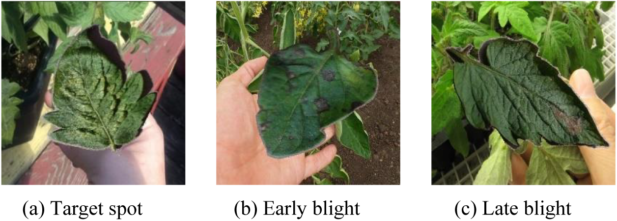
Figure 8: Sample of misclassified images of tomato plant leaves

5.5 Model Performance

The performance of the implemented models is evaluated for each class individually and in average for all classes.

5.5.1 Classwise Performance of Swift-Lite-CvT for 13 Class Classification

Using the confusion matrix shown in Table 9, the precision, recall, and F1 score for the “Swift-Lite-CvT” model were calculated for 13-class classification. The values obtained are presented in Table 10. It is evident from the Table 10 that values for precision and recall are more than 90% for all the classes except early blight, late blight, and target spot. Also, the F1 score varies from 93% to 98% except in the above-mentioned three classes. This is due to the similarity in disease symptoms and the highest number of misclassifications. In contrast, the highest values of precision, recall, and F1 score are reported for Healthy, and Gray Spot classes. The performance of the remaining classes is comparable to each other.

5.5.2 Average Performance of DL Models

In this section, we illustrate the average precision, recall, accuracy, and F1 score of VGG16, ViT, CvT, and Swift-Lite-CvT models applied for 10, 11, and 13 class classifications. We also showcase the training time and storage space required by these models. The comparison in average precision, recall, F1 score, and accuracy for all the above-stated models is shown in Table 11.

It is evident from Table 11 that the Swift-Lite-CvT model achieved an accuracy of 93.51%. It surpasses the 90.4% accuracy of the basic CvT architecture. It is also apparent from Table 11 that the accuracy of all the models viz. VGG 16, ViT, CvT, and Swift-Lite-CvT decreases with an increase in a number of classes. The decrease is due to the availability of a smaller number of training samples for classes such as gray spot, black mold, and powdery mildew. The precision of the Swift-Lite-CvT model decreases with an increase in a number of classes. This is due to the increase in data imbalance. In 13 class datasets, there are 67, 53, and 125 images for gray spot, black mold, and powdery mildew, respectively. This adversely affects the training of the model. However, we increased the number of samples by data augmentation, the number of training samples is 3900, 1004, and 428 for 10 class, 11 class, and 13 class, respectively. The variation in a number of training samples leads to variation in the precision of the model. Additionally, we observed that the proposed model requires storage of 5.8 MB. The storage requirement ratio of the Swift-Lite-CvT is 1:98 with VGG16, 2:98 with ViT, and 7:92 with CvT. Moreover, the proposed models utilize a training time of 44 min. The training time ratio for the proposed model is 48:51 with VGG16, 26:74 with ViT and 42:57 with CvT model. Thus, it is apparent that the proposed model is time and storage-efficient than state-of-the-art models.

Furthermore, our analysis revealed that increasing the number of classes for training affects the model’s performance. A degradation in accuracy is depicted as the increase in number of classes from 10 to 13 as shown in Table 11. Specifically, when conducting a 10-class classification task, we observed remarkably high accuracy across all implemented models. However, as we transitioned to 11-class and 13-class classification tasks, we observed a decline in accuracy. In order to address this challenge, we proposed the utilization of the transformer architecture for the 13-class classification task. The implementation of this architecture significantly improved results, with an accuracy of 93.51%. Notably, this approach offers the added benefits of reduced storage space requirements and decreased processing time compared to previous models. It is evident from results reported in Fig. 9 that a reduction of 51.12%, 74.12%, and 57.7% in computing time of Swift-Lite-CvT is reported when compared to VGG16, ViT, and CvT models, respectively. Moreover, a reduction of 98.93% 98.33%, and a 92.64% in storage space of Swift-Lite-CvT is reported when compared to VGG16, ViT, and CvT models.

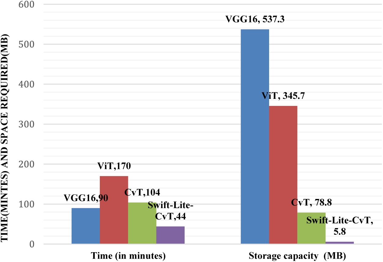
Figure 9: Comparison in storage space and computation time required by the implemented deep learning and transformer models

5.6 Comparative Analysis

To further validate the effectiveness of the Swift-Lite-CvT model, we conducted a comprehensive performance comparison with models applied in the literature for the detection of tomato diseases [51–53]. For instance, the models proposed in references [32–34] achieved comparable accuracies of 96.30%, 99.64%, and 98.05%, respectively. These models utilized a combination of CNN and transformer architectures for 10 class classification. Similarly, Hossain et al., as outlined in reference [54], applied a ViT transformer model with 11 classes and attained an accuracy of 97%, aligning closely with the performance of our proposed model. However, it is noteworthy that the accuracy experienced a decline of 6% as the number of classes increased to 13. The comparison is illustrated in Table 12.

In our investigation, we found out that the Swift-Lite-CvT model has reached its highest accuracy of 99.45% in the case of 10 class classification. Also, it maintains a commendable accuracy of 96.45% in the 11-class classification and a competitive 93.51% in the 13-class classification. While there is room for improvement in terms of accuracy, it is important to highlight that our model demonstrates a significant reduction in both computation time and storage requirements. This improved efficiency enhances the acceptability of our model in real-life implementation for tomato disease classification.

6  Discussions

The CvT model offers a unique blend of convolutional and transformer elements. Convolutions excel at capturing local spatial details, whereas transformers empower the model to analyze global context. This dual proficiency renders CvT a resilient model for visual tasks, surpassing models that rely solely on one of these two mechanisms. The alterations made in the Swift-Lite-CvT were aimed at enhancingcomputational efficiency while preserving a substantial portion of the model’s representational capacity. Here, a convolutional block is used instead of the linear patch projection as in ViT model. This allows for the extraction of local features and spatial information in a more efficient way, especially when dealing with smaller models. Additionally, replacing positional encoding with a convolutional block helps alleviate the need for explicit encoding of positional information. Convolutional layers inherently capture spatial relationships and patterns, removing the need for separate positional encoding. By decreasing the depth of the transformer blocks and fine tuning the number of attention heads, the Swift-Lite-CvT achieved a notable reduction in training by up to 58% which is approximately two times faster than the original CvT The study highlights advantages such as efficient resource utilization and reduced training time making it suitable for mobile devices.

The study given in this manuscript highlights the effectiveness of the Swift-Lite-CvT model for classifying tomato plant leaves. It achieves high accuracy while demanding significantly less storage space and computational time compared to the ViT model as shown in Fig. 9. The proposed architecture utilizes only 44 min and a mere 5.8 MB of space, marking a remarkable success in the realm of plant leaf disease detection. In this study, modifying the heads and depths in the proposed hybrid transformer architecture makes the model efficient even with a small dataset.

7  Conclusions

In this manuscript, we successfully developed the deep learning model “Swift-Lite-CvT” for accurately classifying diseases using images of tomato leaves. We achieved the objectives of minimizing the storage space, and reducing the training time, and some parameters without compromising the accuracy of the model. The model takes a storage space of 5.8 MB and a training time of 44 min. It proves its applicability in real-life scenarios on mobile devices. Moreover, the ratio of storage space of the proposed model to that of VGG16, ViT, and CvT is 1:98, 2:98, and 7:92, respectively. Also, the training time ratio of the proposed model with VGG16, ViT, and CvT models is 48:51, 26:74, and 42:57, respectively. This justifies the superiority of the proposed model “Swift-Lite-CvT” over the above-mentioned models. The model is efficient in handling versatile datasets comprising images with plain as well as complex backgrounds. The efficacy of the proposed model for 10, 11, and 13 classes as shown in Table 11, proves the robustness of the model. The comparison in VGG16, ViT, CvT, and Swift-Lite-CvT models for 10, 11, and 13 classes shows the highest accuracy achieved for 10-class classification. The decrease in accuracy is reported when the number of classes increases from 10 to 11, and 13. The decrease is due to data imbalance and availability of merely 67, 53, and 125 training samples in the original dataset for gray spot, black mold, and powdery mildew classes, respectively. Among all the above-mentioned models, ViT reported the highest accuracy of 96.66%, it utilized a substantial amount of storage space 345.7 MB and a training time of 170 minutes. In contrast, the Swift-Lite-CvT model achieved a comparable accuracy of 93.51%, utilized a storage space of 5.8 MB and a training time of 44 minutes. This plain and compact model can be easily integrated with a mobile or web application and can be implemented in real-life scenarios for classifying tomato leaf diseases. It can also be implemented using IoT-enabled devices, integrated with a user interface for real-time monitoring of tomato fields, and disease detection at an early stage.

Acknowledgement: We acknowledge the lab support given by Manipal University Jaipur in carrying out this research.

Funding Statement: This work is supported by the Department of Informatics, Modeling, Electronics and Systems (DIMES), University of Calabria (Grant/Award Number: SIMPATICO_ZUMPANO).

Author Contributions: All authors contributed equally to the study, conception, design, experiments, manuscript writing, and preparation of the manuscript. All authors reviewed and approved the final version of the manuscript.

Availability of Data and Materials: The data with annotations is available with the authors. We will make the data available after receiving review comments for the manuscript.

Conflicts of Interest: The authors declare that they have no conflicts of interest to report regarding the present study.

References

1. S. C. François-Xavier Branthôme, and Madeleine Royère-Koonings, “tomato online conference,” Parma, Italy, 2020. Accessed: Jan. 17, 2024. [Online]. Available: https://www.tomatonews.com/en/worldwide-total-fresh-tomato-production-exceeds-187-million-tonnes-in-2020_2_1565.html [Google Scholar]

2. Worldostats team, “Tomato Production by Country 2023,” 2023, Accessed: Mar. 27, 2024. [Online]. Available: https://www.worldostats.com/post/tomato-production-by-country-2023 [Google Scholar]

3. L. More, “Business standard,” pp. 1–7, 2021. Accessed: Oct. 18, 2023. [Online]. Available: https://timesofindia.indiatimes.com/potato-and-tomato-output-projected-to-be-down-by-4-5-pc-in-2021-22-govt-data/articleshow/95124336.cms [Google Scholar]

4. S. Keelery, “Production volume of tomatoes,” Statista, 2023. Accessed: Aug. 24, 2024. [Online]. Available: https://www.statista.com/statistics/1039712/india-production-volume-of-tomatoes/ [Google Scholar]

5. J. van Heghe and C. Sirois, “Tomato Processing Market: Global Industry Trends, Share, Size, Growth, Opportunity and Forecast 2023–2028,” 2023, Accessed: Dec. 23, 2023. [Online]. Available: https://www.giiresearch.com/report/imarc1206560-tomato-processing-market-global-industry-trends.html? [Google Scholar]

6. International Market Analysis Research and Consulting Group, “Tomato Processing Market: Industry Trends & Forecast 2024-2032,” 2023, Accessed: Dec. 22, 2023. [Online]. Available: https://www.imarcgroup.com/tomato-processing-plant [Google Scholar]

7. P. S. C. Shivani Machha, N. Jadhav, and H. Kasar, “Crop leaf disease diagnosis using convolutional neural network,” Int. J. Trend Sci. Res. Dev., vol. 4, no. 2, pp. 1056–1058, 2020. [Google Scholar]

8. M. Kaur, B. Varalakshmi, M. Pitchaimuthu, and B. Mahesha, “Screening Luffa germplasm and advanced breeding lines for resistance to Tomato leaf curl New Delhi virus,” J. Gen. Plant Pathol., vol. 87, no. 5, pp. 287–294, Sep. 2021. doi: 10.1007/s10327-021-01010-z. [Google Scholar] [CrossRef]

9. S. Panno et al., “A review of the most common and economically important diseases that undermine the cultivation of tomato crop in the mediterranean basin,” Agronomy, vol. 11, no. 11, pp. 1–45, 2021. doi: 10.3390/agronomy11112188. [Google Scholar] [CrossRef]

10. L. Li, S. Zhang, and B. I. N. Wang, “Plant disease detection and classification by deep learning–A review,” IEEE Access, vol. 9, pp. 56683–56698, 2021. doi: 10.1109/ACCESS.2021.3069646. [Google Scholar] [CrossRef]

11. J. Liu and X. Wang, “Early recognition of tomato gray leaf spot disease based on MobileNetv2-YOLOv3 model,” Plant Methods, vol. 16, no. 1, pp. 1–16, 2020. doi: 10.1186/s13007-020-00624-2. [Google Scholar] [PubMed] [CrossRef]

12. V. S. Dhaka et al., “A survey of deep convolutional neural networks applied for prediction of plant leaf diseases,” Sensors, vol. 21, no. 14, pp. 4749, Jul. 2021. doi: 10.3390/S21144749. [Google Scholar] [PubMed] [CrossRef]

13. S. Mohanty, “Plant Village Dataset,” 2018, Accessed: Dec. 22, 2023. [Online]. Available: https://github.com/spMohanty/PlantVillage-Dataset [Google Scholar]

14. S. P. Mohanty, D. P. Hughes, and M. Salathé, “Using deep learning for image-based plant disease detection,” Front. Plant Sci., vol. 7, no. September, pp. 1–10, 2016. doi: 10.3389/fpls.2016.01419. [Google Scholar] [PubMed] [CrossRef]

15. K. P. Ferentinos, “Deep learning models for plant disease detection and diagnosis,” Comput. Electron. Agric., vol. 145, pp. 311–318, 2018. doi: 10.1016/j.compag.2018.01.009. [Google Scholar] [CrossRef]

16. J. G. A. Barbedo, “Factors influencing the use of deep learning for plant disease recognition,” Biosyst. Eng., vol. 172, no. 660, pp. 84–91, 2018. doi: 10.1016/j.biosystemseng.2018.05.013. [Google Scholar] [CrossRef]

17. L. Yuan et al., “Tokens-to-token ViT: Training vision transformers from scratch on ImageNet,” in Proc IEEE Int. Conf. Comput. Vis., vol. 30, pp. 538–547, 2021. doi: 10.1109/ICCV48922.2021.00060. [Google Scholar] [CrossRef]

18. H. Wu et al., “CvT: Introducing convolutions to vision transformers,” in Proc. IEEE Int. Conf. Comput. Vis., vol. 6, pp. 22–31, 2021. doi: 10.1109/ICCV48922.2021.00009. [Google Scholar] [CrossRef]

19. Daphne Cornelisse, “An intuitive guide to Convolutional Neural Network,” 2018, Accessed: Dec. 22, 2023. [Online]. Available: https://www.freecodecamp.org/news/an-intuitive-guide-to-convolutional-neural-networks-260c2de0a050/ [Google Scholar]

20. J. G. Arnal Barbedo, “Plant disease identification from individual lesions and spots using deep learning,” Biosyst. Eng., vol. 180, pp. 96–107, 2016. doi: 10.1016/j.biosystemseng.2019.02.002. [Google Scholar] [CrossRef]

21. P. Kaur et al., “Recognition of leaf disease using hybrid convolutional neural network by applying feature reduction,” Sensors 2022, vol. 22, no. 2, pp. 575, Jan. 2022. doi: 10.3390/S22020575. [Google Scholar] [PubMed] [CrossRef]

22. R. Thangaraj, S. Anandamurugan, P. Pandiyan, and V. K. Kaliappan, “Artificial intelligence in tomato leaf disease detection: A comprehensive review and discussion,” J. Plant. Dis. Prot., vol. 129, no. 3, pp. 469–488, 2022. doi: 10.1007/s41348-021-00500-8. [Google Scholar] [CrossRef]

23. M. Agarwal, A. Singh, S. Arjaria, A. Sinha, and S. Gupta, “ToLeD: Tomato leaf disease detection using convolution neural network,” Procedia Comput. Sci., vol. 167, pp. 293–301, 2020. doi: 10.1016/j.procs.2020.03.225. [Google Scholar] [CrossRef]

24. I. Ahmad, M. Hamid, S. Yousaf, S. T. Shah, and M. O. Ahmad, “Optimizing pretrained convolutional neural networks for tomato leaf disease detection,” Complexity, vol. 2020, pp. 1–6, 2020. doi: 10.1155/2020/8812019. [Google Scholar] [CrossRef]

25. L. Norria, S. Ricky, and A. Nazari, “Tomato leaf disease detection using convolution neural network (CNN),” Evol. Electr. Electron. Eng., vol. 2, no. 2, pp. 667–676, Nov. 2021. doi: 10.30880/eeee.2021.02.02.080. [Google Scholar] [CrossRef]

26. M. E. H. Chowdhury et al., “Automatic and reliable leaf disease detection using deep learning techniques,” AgriEngineering, vol. 3, no. 2, pp. 294–312, 2021. doi: 10.3390/agriengineering3020020. [Google Scholar] [CrossRef]

27. V. Gonzalez-Huitron, J. A. León-Borges, A. E. Rodriguez-Mata, L. E. Amabilis-Sosa, B. Ramírez-Pereda and H. Rodriguez, “Disease detection in tomato leaves via CNN with lightweight architectures implemented in Raspberry Pi 4,” Comput. Electron. Agric., vol. 181, pp. 105951, 2021. doi: 10.1016/j.compag.2020.105951. [Google Scholar] [CrossRef]

28. S. M. Hassan, A. K. Maji, M. Jasiński, Z. Leonowicz, and E. Jasińska, “Identification of plant-leaf diseases using cnn and transfer-learning approach,” Electron., vol. 10, no. 12, pp. 1388, 2021. doi: 10.3390/electronics10121388. [Google Scholar] [CrossRef]

29. A. Abbas, S. Jain, M. Gour, and S. Vankudothu, “Tomato plant disease detection using transfer learning with C-GAN synthetic images,” Comput. Electron. Agric., vol. 187, pp. 106279, 2021. doi: 10.1016/j.compag.2021.106279. [Google Scholar] [CrossRef]

30. C. Zhou, S. Zhou, J. Xing, and J. Song, “Tomato leaf disease identification by restructured deep residual dense network,” IEEE Access, vol. 9, pp. 28822–28831, 2021. doi: 10.1109/ACCESS.2021.3058947. [Google Scholar] [CrossRef]

31. A. S. Paymode and V. B. Malode, “Transfer learning for multi-crop leaf disease image classification using convolutional neural network VGG,” Artif. Intell. Agric., vol. 6, no. 2, pp. 23–33, 2022. doi: 10.1016/j.aiia.2021.12.002. [Google Scholar] [CrossRef]

32. T. Vadivel and R. Suguna, “Automatic recognition of tomato leaf disease using fast enhanced learning with image processing,” Acta Agric. Scand. Sect. B Soil Plant Sci., vol. 72, no. 1, pp. 312–324, 2022. doi: 10.1080/09064710.2021.1976266. [Google Scholar] [CrossRef]

33. H. Tarek, H. Aly, S. Eisa, and M. Abul-Soud, “Optimized deep learning algorithms for tomato leaf disease detection with hardware deployment,” Electron., vol. 11, no. 1, pp. 1–19, 2022. doi: 10.3390/electronics11010140. [Google Scholar] [CrossRef]

34. Y. Wang, Y. Chen, and D. Wang, “Convolution network enlightened transformer for regional crop disease classification,” Electron., vol. 11, no. 19, pp. 3174, Oct. 2022. doi: 10.3390/ELECTRONICS11193174. [Google Scholar] [CrossRef]

35. S. Yu, L. Xie, and Q. Huang, “Inception convolutional vision transformers for plant disease identification,” Internet of Things, vol. 21, no. 288, pp. 100650, 2023. doi: 10.1016/j.iot.2022.100650. [Google Scholar] [CrossRef]

36. D. P. Hughes and M. Salathe, “An open access repository of images on plant health to enable the development of mobile disease diagnostics,” arXiv:1511.08060, 2015. [Google Scholar]

37. MIT, “iBean,” Makerere AI Lab, 2020, Accessed: Jan. 20, 2020. [Online]. Available: https://github.com/AILab-Makerere/ibean/blob/master/README.md [Google Scholar]

38. S. Huang, W. Liu, F. Qi, and K. Yang, “Development and validation of a deep learning algorithm for the recognition of plant disease,” in Proc. 21st IEEE Int. Conf. High Perform. Comput. Commun.; 17th IEEE Int. Conf. Smart City; 5th IEEE Int. Conf. Data Sci. Syst. (HPCC/SmartCity/DSS), 2019, pp. 1951–1957. doi: 10.1109/HPCC/SmartCity/DSS.2019.00269. [Google Scholar] [CrossRef]

39. D. Singh, N. Jain, P. Jain, P. Kayal, S. Kumawat and N. Batra, “PlantDoc: A dataset for visual plant disease detection,” in ACM Int. Conf. Proceeding Ser., 2020, pp. 249–253. doi: 10.1145/3371158. [Google Scholar] [CrossRef]

40. M. S. Alzahrani and F. W. Alsaade, “Transform and deep learning algorithms for the early detection and recognition of tomato leaf disease,” Agronomy, vol. 13, no. 5, pp. 1184, 2023. doi: 10.3390/agronomy13051184. [Google Scholar] [CrossRef]

41. W. Bao, X. Huang, G. Hu, and D. Liang, “Identification of maize leaf diseases using improved convolutional neural network,” Nongye Gongcheng Xuebao/Transactions Chinese Soc. Agric. Eng., vol. 37, no. 6, pp. 160–167, 2021. doi: 10.11975/j.issn.1002-6819.2021.06.020. [Google Scholar] [CrossRef]

42. L. Li, S. Zhang, and B. Wang, “Apple leaf disease identification with a small and imbalanced dataset based on lightweight convolutional networks,” Sens., vol. 22, no. 1, pp. 173, 2022. doi: 10.3390/s22010173. [Google Scholar] [PubMed] [CrossRef]

43. Abdallah Ali, “PlantVillage Dataset,” 2019, Accessed: Dec. 25, 2023. [Online]. Available: https://www.kaggle.com/datasets/abdallahalidev/plantvillage-dataset [Google Scholar]

44. Y. H. Huang and M. L. Chang, “Dataset of tomato leaves,” Mendeley Data, 2020. doi: 10.17632/ngdgg79rzb.1. [Google Scholar] [CrossRef]

45. Nirmal Sankalana, “PlantDoc Classification dataset,” 2020, Accessed: Dec. 25, 2023. [Online]. Available: https://www.kaggle.com/datasets/nirmalsankalana/plantdoc-dataset [Google Scholar]

46. K. Simonyan and A. Zisserman, “Very deep convolutional networks for large-scale image recognition,” in 3rd Int. Conf. Learn. Represent., 2015, pp. 1–14. [Google Scholar]

47. S. H. Lee, H. Goëau, P. Bonnet, and A. Joly, “New perspectives on plant disease characterization based on deep learning,” Comput. Electron. Agric., vol. 170, pp. 105220, 2020. doi: 10.1016/j.compag.2020.105220. [Google Scholar] [CrossRef]

48. S. J. Jia, P. Y. Jia, S. P. Hu, and H. B. Liu, “Automatic detection of tomato diseases and pests based on leaf images,” in Proc. 2017 Chinese Autom. Congr. (CAC), 2017, pp. 2510–2537. doi: 10.1109/CAC.2017.8243388. [Google Scholar] [CrossRef]

49. A. Dosovitskiy et al., “An image is worth 16 × 16 words: Transformers for image recognition at scale,” arXiv:2010.11929, 2020. [Google Scholar]

50. K. He, X. Zhang, S. Ren, and J. Sun, “Deep residual learning for image recognition,” in Proc IEEE Comput. Soc. Conf. Comput. Vis. Pattern Recognit, 2016, pp. 770–778. doi: 10.1109/CVPR.2016.90. [Google Scholar] [CrossRef]

51. M. L. Gleason and B. A. Edmunds, “Tomato diseases and disorders,” Instructional Technology Center, Iowa State University, pp. 1–12, 2006, Accessed: Mar. 26, 2024. [Online]. Available: https://ncmg.ucanr.org/files/180088.pdf. [Google Scholar]

52. S. Kaur, S. Pandey, and S. Goel, “Plants disease identification and classification through leaf images: A survey,” Arch. Comput. Methods Eng., vol. 26, no. 2, pp. 507–530, 2019. doi: 10.1007/s11831-018-9255-6. [Google Scholar] [CrossRef]

53. H. Waghmare, R. Kokare, and Y. Dandawate, “Detection and classification of diseases of Grape plant using opposite colour Local Binary Pattern feature and machine learning for automated Decision Support System,” in 2016 3rd Int. Conf. Signal Process. Integr. Netw. (SPIN), Noida, India, 2016, pp. 513–518. doi: 10.1109/SPIN.2016.7566749. [Google Scholar] [CrossRef]

54. S. Hossainet al., “Aggregating different scales of attention on feature variants for tomato leaf disease diagnosis from image data: A transformer driven study,” Sensors, vol. 23, no. 7, pp. 3751, Apr. 2023. doi: 10.3390/S23073751. [Google Scholar] [PubMed] [CrossRef]