Collaborative Charging Scheduling in Wireless Charging Sensor Networks

1  Introduction

Wireless sensor networks are composed of randomly distributed sensor nodes. Each sensor node has a different monitoring task and transmits the sensed data to the base station. The battery energy of sensor nodes in wireless sensor networks is limited [1,2], and the network lifetime is usually limited. In recent years, many solutions have been proposed by researchers to solve this problem. One solution is to conserve network energy consumption through optimization methods, such as data fusion algorithms [3], layered routing protocols [4], and clustering algorithms [5]. Although these methods extend the network lifespan to a certain extent, the limited lifespan of sensor node batteries still hinders the large-scale deployment of wireless sensor networks. Another solution is to actively seek energy supplementation for WSNs, such as renewable energy technology that converts solar and thermal energy into electricity [6,7], but the energy collected from the environment is uncontrollable.

Wireless power transmission (WPT) system generally consists of a high-frequency power supply, load driving circuit, impedance, resonant coil, and induction coil. The principle is to make the magnetic resonance coils at the transmitting and receiving ends have the same resonance frequency so that the energy generated by the high-frequency power supply can be transmitted from the transmitting coil to the receiving coil through a non-radiative magnetic field [8]. Wireless rechargeable sensor networks have gradually attracted attention with the development of WPT. In the network, mobile chargers are integrated and replenish stable and efficient energy for sensors with insufficient energy, which largely overcomes the issue of sensor energy shortage caused by environmental or human factors.

In actual scenarios, the residual energy and energy consumption of sensors typically differ. For instance, in the cluster network structure, the cluster head and its neighboring sensor nodes transfer a greater amount of data compared to other sensors, leading to higher energy consumption. The MC has a limited capacity and may not be able to replenish energy for all sensors during a charging trip. It is essential to establish a sensible charging schedule to address the charging requirements of the sensor nodes and prevent sensor failure due to energy exhaustion. To solve the problem, He et al. [9] proposed the Nearest Job Next with Preemption algorithm (NJNP), in which the charging request of the sensor closest to MC is the first to be responded to, but the sensors that are too far away from the MC may not get energy supplement in time; In the first come first serve (FCFS) algorithm [10], the sensor that sends the charging request first is served first, but this approach results in the MC consuming a significant amount of energy during charging traveling. In the invalid node minimized algorithm (INMA) algorithm [11], the sensor node with the shortest charging time is selected as the next charging node, but the cost is high. The Temporal and Distantial Priority (TADP) algorithm [12] selects the sensor with the highest mixed priority as the charging node. The priority is determined by the arrival time of charging requests and the distance. TADP algorithm ignores the changes in node energy consumption and the energy limitations of MC. In the Charging Scheduling Scheme that Maximizes Energy Efficiency (CSS-MEE) algorithm [13], the sensor node that can maximize the charging utility will become the next charging node. However, multiple MCs cannot charge collaboratively for sensor nodes.

Many previous studies have assumed ideal application prerequisites, such as sensor nodes in the network having uniform energy consumption rates, MC having sufficient energy to meet all charging requests, and so on. This has resulted in an overly vague and imprecise selection of charging nodes and partial charging capacity settings. Motivated to overcome the existing problems mentioned above, we aim to present a novel on-demand charging strategy that is guided by the advantages of existing designs while minimizing the impacts of their limitations. The contributions of this work can be summarized as follows:

• To effectively adapt to the dynamic nature of on-demand charging, we propose an efficient scheme which employs a dynamic charging scheduling strategy and dynamically adjusts the energy thresholds of the sensor nodes.

• To improve the survival rate of sensor nodes, we employ two MCs for cooperative charging, and the two MCs can adaptively change the charging method in real time according to the energy of the MCs and the sensor charging request.

•The performance of our proposed scheme is evaluated through MATLAB simulations. Simulation results demonstrate that our scheme achieves better performance compared to other algorithms.

The rest of the paper is organized as follows: Related works are discussed in Section 2. Section 3 describes the network model, charging model, and problem definition. The collaborative charging scheduling algorithm is proposed in Section 4. Experimental results are presented in Section 5. Section 6 is for discussion. Finally, Section 7 concludes our paper.

2  Related Works

In recent years, the research on WRSN has gradually increased in popularity. In WRSNs, one or more MCs are equipped to supplement energy for sensor nodes. According to the type of charging scheduling, recent studies are divided into periodic charging and on-demand charging.

In the periodic charging strategy, one or more MCs complete the energy supplement task according to the predetermined charging schedule. After a certain period, MCs will repeat the previous charging traveling to charge these sensor nodes. This scheme assumes that the energy consumption rate of sensors during network operation is predictable and constant. Ye et al. [14] proposed an approximate algorithm for a closed charging path and a heuristic algorithm for traversing the minimum spanning tree. Both algorithms are suitable for smaller networks. Xie et al. [15] proposed that the optimal charging path of MC is the shortest Hamiltonian cycle, and the approximate optimal solution is obtained by piecewise linear approximation under the condition that idle time and running time are maximized. Guo et al. [16] aimed to minimize the charging time by concurrent charging scheduling, and presented two greedy charging scheduling algorithms. Chen et al. [17] proposed a two-sided charging strategy for MC traversal planning, which minimizes the energy consumption, charging path, and travel time of MC. Li et al. [18] introduced a weighted value between the amount of sensor data loss and the traveling distance of MC to calculate the amount of data loss based on static routing and dynamic routing. The method attempts to achieve a balance between minimizing the traveling distance of MC and data loss in WRSNs. Shan et al. [19] proposed an intelligent path optimization algorithm based on intelligent algorithms and deep reinforcement learning, which have some advantages in planning charging paths for unmanned aerial vehicles in small and medium-sized networks. Soni et al. [20] used mobile charging equipment and fixed charging equipment to charge key sensor nodes and common sensor nodes, respectively, and optimize the charging path by using the reinforcement learning algorithm.

In practical application scenarios, the attributes of WRSN sensors are constantly changing, and the offline periodic charging strategy cannot adapt to these changes, which may compromise network performance. In contrast, the dynamic nature of on-demand charging is more in line with the needs of the service order of sensors in the charging pool is variable. The charging scheduling method of MC plays a crucial role in improving charging efficiency. Chen et al. [13] introduced an adaptive construction path and a preemption mechanism for the sensor. When the network scale becomes larger, the available energy of MC is far less than the requested charging energy. It requires multiple MCs to work together and divides the large area into reasonable small areas. Dong et al. [21] proposed a demand-based charging strategy (DBCS) and a dynamically selecting charging node algorithm (DSACN), which achieved good performance in reducing the length of the charging path. However, the impact of dynamic energy consumption rates on charging selection was not considered Lin et al. [22] proposed double warning thresholds with a double preemption (DWDP) charging scheme, where the charging sequence is determined according to the emergency level of the sensor. However, after the algorithm was used for network partitioning, the charging scheduling problem in its overlapping areas was not solved. Dong et al. [23] proposed an instant-on-demand billing strategy (IOCS) which divided the network area into multiple subregions based on the enhanced K-means algorithm, and each subregion is assigned an MC to charge the sensors. The proposed strategy effectively balances the network load, but lacks collaboration with MC, resulting in high overhead. Tang et al. [24] proposed a scheme for replenishing the sensor nodes and routing under specific charging conditions based on MC’s energy supply capacity, the sensor’s residual energy, and energy consumption intensity. Sheikhi et al. [25] used virtual areas to partition the entire network. Each mobile charger belongs to a different virtual area. When the MC moves, it sends a broadcast message. If other sensor nodes to be charged have the highest interest in the MC, they will respond. The scheme effectively shortens the traveling distance, but the cost is higher. Alkhalidi et al. [26] divided the entire network into equally spaced rings. Each ring includes multiple sectors. After the sensor nodes in the sector send the charging request to the base station, the base station calculates the location of the sensor’s sector. The sector with the maximum number of charging sensors has the highest service priority, but the charging fairness of this scheme cannot be guaranteed. Priyadarshani et al. [27] generated the optimal charging sequence for MC by identifying the halting point. However, the study did not consider the impact of energy consumption rate on charging location and charging volume. Wang et al. [28] introduced the optimal charging rate and calculated it according to the overall sensor survival rate, effectively extending the network lifetime. However, the proposed partial charging scheme lacks fairness for sensor nodes.

Considering the relevant factors in practical network applications, such as the dynamic energy consumption rate of sensor nodes, the constraints of a single MC, and the limited capacity of MC batteries, we propose a collaborative charging scheduling algorithm that fully takes into account the dynamic energy consumption of nodes and the collaborative challenges of multiple MCs. Meanwhile, we propose to utilize dynamic thresholds and partial charging to adapt to network changes more effectively.

3  Modeling and Problem Formulation

3.1 Network Model

M homogeneous sensor nodes equipped with one rechargeable battery of capacity Em are deployed in an L × L area randomly. At time t = 0, all sensor nodes in the network have full battery capacity. Each sensor node is equipped with a wireless power receiver to obtain energy from the MC. These sensor nodes have different energy consumptions due to their different monitoring tasks. Sensor nodes send data to the base station every Δ. To balance the energy consumption of wireless sensor networks, the whole network is clustered according to the K-means method [29], and each cluster head node is located near the center of its cluster. The base station is located at the center of the WRSN. The base station is in charge of processing the information sent by the sensor nodes, as well as the energy supplement and maintenance of MC. The initial position of the MCs is at the base station, and the battery capacity of the MCs is Ew. When the residual energy of the sensor node ni reaches the threshold Eth, it will send a charging request to the base station. After receiving the charging request message, the base station will forward the charging request to MC by remote communication. The MC has powerful computing capability and communication capability to maintain the charging request service pool. The MC charges the sensor nodes in the service pool in a one-to-one manner according to the scheduling sequence. When the MC has insufficient energy to charge the next sensor node, it will return to the base station for replenishment. The network model is shown in Fig. 1.

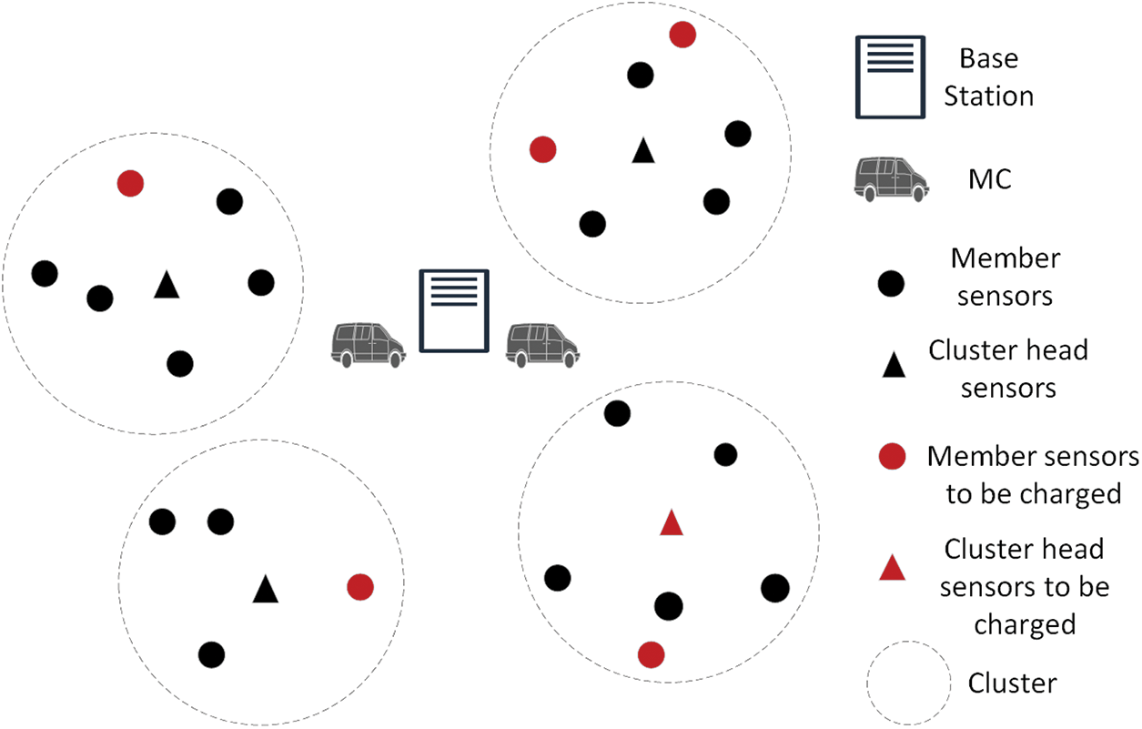
Figure 1: Network model

3.2 Charging Model

The WRSN charging model in the paper refers to the literature [30], which is expressed as follows:

Pt=GtGrwLp(λ4π)2Ps,(1)

Pr=Pt(dx+β)2,(2)

where Ps is the power of the MC transmission antenna, Pr is the power of the sensor node receiving energy, Gt is the source antenna gain, Gr is the receiver antenna gain, w is the rectifier efficiency, Lp is the polarization loss, λ is the wavelength, β is the adjustable parameter of the Frith transfer formula, dx is the Euclidean distance between the sensor node and MC.

3.3 Problem Description

Assumption 1: The energy consumption generated by sensor nodes when sending charging requests is neglected, and Em remains unchanged during network operation. The sensor node can maintain normal functionality during the charging process, including perception and communication.

Assumption 2: MC charging mode is one-to-one charging. When its residual energy cannot meet the demand of the next charging sensor, MC will return to the base station for energy supplement.

For a sensor node ni, there is a minimum energy Ed. When the residual energy of the sensor node reaches Eth(Eth>Ed), the sensor will send a charging request. After the sensor node sends a charging request, it reaches the minimum energy Ed before receiving an energy supplement, the sensor will enter the half-asleep state and will not participate in monitoring tasks in the network, but can transmit and receive information normally. To ensure the normal operation of the network, two MCs are reasonably scheduled to charge the sensors in the charging request pool. Assume that the number of surviving sensors is Us and the number of dead sensors is Ud during network operation. When the remaining energy of the sensor node reaches Ed, it is marked as a dead node. Pu represents the proportion of dead sensors in the network, the charging scheduling problem can be described as follows:

Pu=UdUd+Us,(3)

min(Pu).(4)

s.t.∑i=0PEni+Etl<Ew,(5)

Er,i≤REi.(6)

Eqs. (3) and (4) indicate that the goal of the charging scheduling algorithm is to minimize the number of dead sensors. Eq. (5) indicates that the energy consumed by MC during a single charging traveling cannot exceed its maximum battery capacity. Eni is the energy replenished by MC for the sensor ni, and P is the charging request amount, Etl represents the energy consumed by MC during its traveling from the base station to its return. Eq. (6) indicates that the energy consumed by the sensor node ni at any time cannot exceed its residual energy.

4  Charging Scheduling Algorithm

4.1 Classification of Charging Sensors

The sensor nodes in the network undertake different monitoring tasks and transmit different data flows, and the energy consumed per unit time will also be different. At the beginning of the network operation, the K-means-based clustering method is used to cluster. The cluster head is located near the center of the whole cluster and receives and fuses the information from the member sensors in the cluster, and then forwards it to the base station, which will make the cluster head consume more energy. Therefore, a certain number of candidate cluster heads should also be selected to ensure the smooth operation of the whole cluster. Assuming that the radius of a cluster is r, the cluster head is in the center, and all the sensors within the 0.2r range have the opportunity to become the cluster head. Whenever the energy of the cluster head reaches 1.5Eth, the next cluster head is selected from the candidate cluster heads. The principle of cluster head selection is that the candidate cluster head with the highest matching degree Pi will become the next cluster head. The matching degree Pi of candidate cluster head ni is given by:

Pi=αREi(t)+(1−α)di(7)

where REi(t) denotes the residual energy of the current sensor, di denotes the distance from the sensor’s current position to the cluster head. α is the weight, α∈[0,1]. The weight value may be different for different clusters. For example, in a cluster with large energy consumption, the larger α makes the residual energy factor occupy more proportion, which is beneficial to the stable operation of the cluster. But if α is too large, the cluster head in the next round will be away from the center, and sensor nodes far from the cluster head will have higher energy consumption communicating with the cluster head.

An appropriate cluster head rotation mechanism can prolong the network life, but the residual energy of the cluster head and candidate cluster head will eventually drop to the threshold, if these critical sensor nodes cannot be replenished in time, the network failure will occur, so the network needs MC to replenish energy for sensor nodes. Sensor nodes in the same cluster have some common attributes, such as the monitoring target and the amount of data forwarded, so the energy consumption rate of member sensor nodes in the same cluster will be very close, which makes the charging path of MC shorter. The base station divides the charging sensor nodes into important sensor nodes and ordinary sensor nodes, the important sensor nodes include cluster heads and candidate cluster heads, and the ordinary sensor nodes are other member sensor nodes. MC1 only charges the important sensor nodes, while MC2 charges ordinary sensor nodes in the network except important sensor nodes. Whenever the residual energy of the sensor nodes decreases to Eth, the charging request messages will be sent to the base station, including ID, member property, and the location of the sensor. Upon receiving the request, the base station will analyze and process it, and then forward it to the corresponding MC according to the member property. The MC will store it in the service pool and select the next charging node in the service pool based on the charging scheduling order.

4.2 Charging Node Selection

Whenever the residual energy of the sensor node ni reaches the threshold Eth, it will send a charging request to the base station, which will process the message and forward it to the MC. The message will be stored in the charging request service pool of MC, and MC will provide charging services for the nodes in the service pool according to the scheduling order. Some literature [31,32] only take the residual energy of sensor nodes as a consideration factor, but in actual network operation, due to the changes of monitoring object, monitoring environment, and other factors, the energy consumption of sensor nodes is dynamic during the working period. With the gradual stabilization of the network operation, the energy consumption rate will decrease. Some sensor nodes may have a large energy consumption rate due to the change of the monitoring target or the increase of forwarding data flow. Therefore, it is necessary to consider the real-time energy consumption rate of the sensor node to estimate the remaining life of the node accurately. It is assumed that sensors send data to the cluster head every Δ, and the cluster head summarizes this information and forwards it to the base station for analysis. The information includes not only the monitored object information, but also the ID, residual energy, and timestamp information of the sensor. Assuming the energy consumption rate of the sensor node ni at time t is Ri(t), then the energy consumption rate Ri(t+Δ) at time t + Δ:

Ri(t+Δ)=βRi(t)+(1−β)REi(t−Δ)−REi(t)Δ,(8)

where REi(t−Δ) and REi(t) represent the residual energy of the sensor node ni at time t−Δ and t, respectively, β is the weight, β ∈ [0,1]. If the object to be monitored in the network is complex, the value of β should be reduced. The survival time Li of sensor ni is expressed as:

Li=REi(t)Ri(t+Δ).(9)

The shorter the life of the sensor node in the charging request pool, the greater the chance of it being the next charging option for MC. When the sensor node is in a charging state, the transmission of this information will be suspended. After the sensor node is fully charged, it will continue to send information to the base station every Δ time interval.

The distance between MC and the sensor in the charging request pool changes dynamically during the charging traveling. If the impact of the distance on MC charging scheduling is ignored, the nearest sensor to MC may not have a chance to get charged, and MC will spend more time and energy on the charging traveling. Therefore, the distance between the sensor to be charged and the MC should become an important factor in charging scheduling. The closer the sensor is to the MC, the greater the chance it will become the next charging sensor of the MC. Assuming that the coordinate of the sensor ni is (Xi,Yi) and the coordinate of MC2 is (Xw2,Yw2), then the Euclidean distance Di between the sensor ni and MC2 is:

Di=(Xi−Xw2)2+(Yi−Yw2)2.(10)

In the cluster network structure, some sensor nodes may be unable to work normally due to battery depletion, which may bring many problems. For instance, a failure of the sensing node may lead to integrity issues with the monitored target data, while a failure of the intermediate node may cause changes in data forwarding paths and consume more energy [33,34]. Therefore, when selecting the sensor node to be charged, the position of the sensor nodes within the cluster should be taken into account. The sensor node with a higher number of child nodes Ni that need to be charged plays a more important role within the cluster, which will have a greater chance of becoming the next charging sensor of MC.

Assuming that the charging demand degree W(i) determines the charging order, the higher the value of W(i), the higher the charging priority of the sensor. Based on the influence of two factors on charging: The life of the sensor and the Euclidean distance between the sensor and MC, the charging demand degree W(i) of the sensor ni is expressed as:

W(i)=xLi+yDi+zNi,(11)

x+y+z=1,(12)

where x, y, and z are the weights of real-time node lifespan Li, Euclidean distance Di between the node and MC, and the number of children nodes Ni, respectively. If the average residual energy of sensor nodes in the network is at a low level, it should be increased by x; If the network nodes are densely distributed, y should be increased; If the data transmission delay needs to be controlled, z should be increased. MC supplements energy to nodes in order based on W(i).

After completing the charging of a sensor node, MC will delete the node’s request from the service pool, and send a request to the base station to update the survival time of the existing sensor nodes in the service pool. The base station will provide MC with the real-time survival time of sensor nodes based on the latest received messages from these sensor nodes. During network operation, both the base station and MC are equipped with high-power communication devices, the base station can directly send the information of the sensor nodes to the MC, allowing the MC to update the survival time of the sensor nodes in the service pool. In addition, the Euclidean distance between sensor nodes and MC is constantly changing, so W(i) value is dynamic. The MC always selects the sensor node with the largest W(i) value in the service pool.

4.3 Dynamic Charging Threshold

When the remaining energy of the sensor node falls below the charging threshold Eth, a charging request is sent to the base station. The value of Eth affects the lifetime of WRSN. If Eth is set too high, the sensors will frequently send charging requests, MC will consume more energy on the charging traveling. If Eth is set too low, it may cause the sensor to enter a sleep state before MC arrives, which will affect the normal operation of the network. To solve this problem, the dynamic energy threshold method is introduced in the literature [35]. The paper improves the dynamic energy threshold to optimize the charging frequency based on the cluster network.

The MC near the base station will go to the sensor for energy replenishment upon receiving a charging request from the sensor node ni. The time required for this process is tmin, which can be expressed as:

tmin=Di,bv,(13)

where Di,b is the Euclidean distance between the sensor node ni and the base station and v is the speed of MC.

To enable the sensor node ni to receive energy replenishment in time, the survival time of the sensor node ni after sending a charging request should be greater than tmin:

Eth≥max[Ri(t+Δ)×tmin].(14)

Each sensor node in the network has its charging latency, which is the waiting time for MC to come to the sensor for charging after the sensor sends a charging request. Assuming the average waiting time of the sensor nodes is tn, tn can be determined as follows:

tn=[Dav+(2Dav+Em−EthPr)+…+(MDav+(M−1)(Em−Eth)Pr]M,(15)

where Da is the average Euclidean distance between sensor nodes, Em−EthPr represents the charging time of MC. The average energy consumption Ra(t + Δ) of sensor nodes during ∆ time can be expressed by Eq. (16):

Ra(t+Δ)=1M∑i=1MRi(t+Δ).(16)

Then Eth should be greater than the average energy consumption Ra(t+Δ):

Eth≥tn×Ra(t+Δ).(17)

At the beginning of the network, the base station calculates the initial energy threshold Eth for the sensor nodes according to Eq. (14) based on the first charging request information. After that, the base station calculates Eth according to Eqs. (14) and (17), respectively, and the charging threshold Eth is determined by the maximum value in Eqs. (14) and (17). To reduce unnecessary energy consumption, we stipulate that when the threshold change is less than 10%, the base station will not update the charging threshold Eth. After the network stabilizes, the charging threshold Eth tends to stabilize.

4.4 Charging Schedule Strategy

After receiving the charging request from the node, the base station performs certain processing and forwards it to either MC1 or MC2. The battery capacity of MC1 and MC2 is equal and limited, and they undertake the charging tasks for different types of sensors. Some sensor nodes fail because they cannot get energy supplements in time. To solve this problem, the paper proposes a cooperative charging strategy with an adaptive feature, which can effectively prolong the network lifetime.

4.4.1 Cooperative Charging Mechanism

In this paper, two MCs charge the sensors one-to-one. MC1 charges the cluster head and its candidate cluster head, while MC2 charges the other member sensors in the cluster. In a clustered network, the number of cluster heads and candidate cluster heads is only a small part of the cluster, so the number of requests in the service pool of MC1 is much smaller than that of MC2, and the charging work undertaken by MC2 is higher than that of MC1. When the MC2 judges that it cannot charge the next sensor, it will return to the base station for energy replenishment, and the sensors in the MC2 service pool may fail during MC2 energy replenishment.

The paper proposes a cooperative charging strategy based on two MCs. When MC2 needs to return to the base station for energy replenishment, it will communicate with MC1, and send a request message to MC1. After receiving the message, MC1 checks whether the service pool is empty. If the pool is empty, it means that the charging task has been completed and there are no sensors to be charged. So, it returns a message to MC2 indicating that it can assist MC2 in completing the charging of the remaining sensors. After receiving the message from MC1, MC2 will send MC1 a message to MC1, including the remaining sensors in the service pool, and MC1 will charge these sensors. MC1 can receive the charging requests forwarded by the base station and prioritize the charging service for these important sensor nodes. Before MC1 completes charging the important sensor nodes, MC2 will service the remaining charging requests of ordinary sensor nodes. MC2 responds with a confirmation message after receiving service requests from ordinary sensor nodes in MC1 and prioritizes charging services for these nodes. Upon receiving a confirmation message, MC1 will remove these sensor nodes from its service pool.

4.4.2 Adaptive Charging Mechanism

The collaborative charging strategy can reduce the death rate of sensor nodes, but it cannot always be effective. It is assumed that MC2 needs to return to the base station and complete the power replenishment, and there are requests in the service pools of MC1 and MC2 at this time. Because the service pool of MC1 is in a non-idle state, ordinary sensor nodes cannot obtain the charging service of MC1. In this case, the cooperative charging mechanism is invalid. It is necessary to partially charge ordinary sensors to ensure that the overall dead of the sensor nodes reaches the minimum because the charging efficiency of the lithium battery decreases gradually with the increase of battery power. When the battery power reaches about 80%, the charging efficiency will drop sharply. It would take a lot of time to fully replenish these ordinary sensor nodes [36], whereas MC can replenish more sensor nodes in the same long time to reduce the overall dead rate of the nodes. Based on the importance of cluster head nodes and their candidate cluster head nodes, MC1 will fully charge these sensor nodes. Once the charging in its service pool exceeds the battery capacity of the MC, the MC2 switches its charging method to partially charge the ordinary sensor nodes. The partial charging capacity consists of two parts: Fixed charging power Efx and adaptive charging power Eap:

Efx=λ(1−Pm)Eth,(18)

where P is the number of charging requests of ordinary sensors, m is the number of ordinary sensors, and λ is the coefficient, which is used to control the fixed charging amount not less than the minimum requirement, λ should not be too high, otherwise Efx may exceed the residual energy of MC. Assume that the minimum power of the sensor after charging is βEth, β > 1, and the current power of MC2 is Ere, then:

Ere>Efx>PβEth.(19)

Eap=Ere−Efx.(20)

The fixed amount of charging allocated to sensor nodes decreases as the number of charging requests increases. The adaptive charging amount Eap of sensor ni is determined according to the life of the sensor node. The life Li of the sensor node means the urgency of the sensor’s charging. The shorter the life of the sensor, the greater the demand for the adaptive charging power. The corresponding adaptive charging power Eap(i) of sensor ni is:

Eap(i)=(Ere−Efx).k.∑iPLiLi,(21)

where k is a factor, k > 0.

The total charge amount Esum of sensor ni in this round is:

Esum=λ(1−Pm).Eth+(Ere−Efx).k.∑iPLiLi.(22)

5  Simulation Outcomes and Analysis

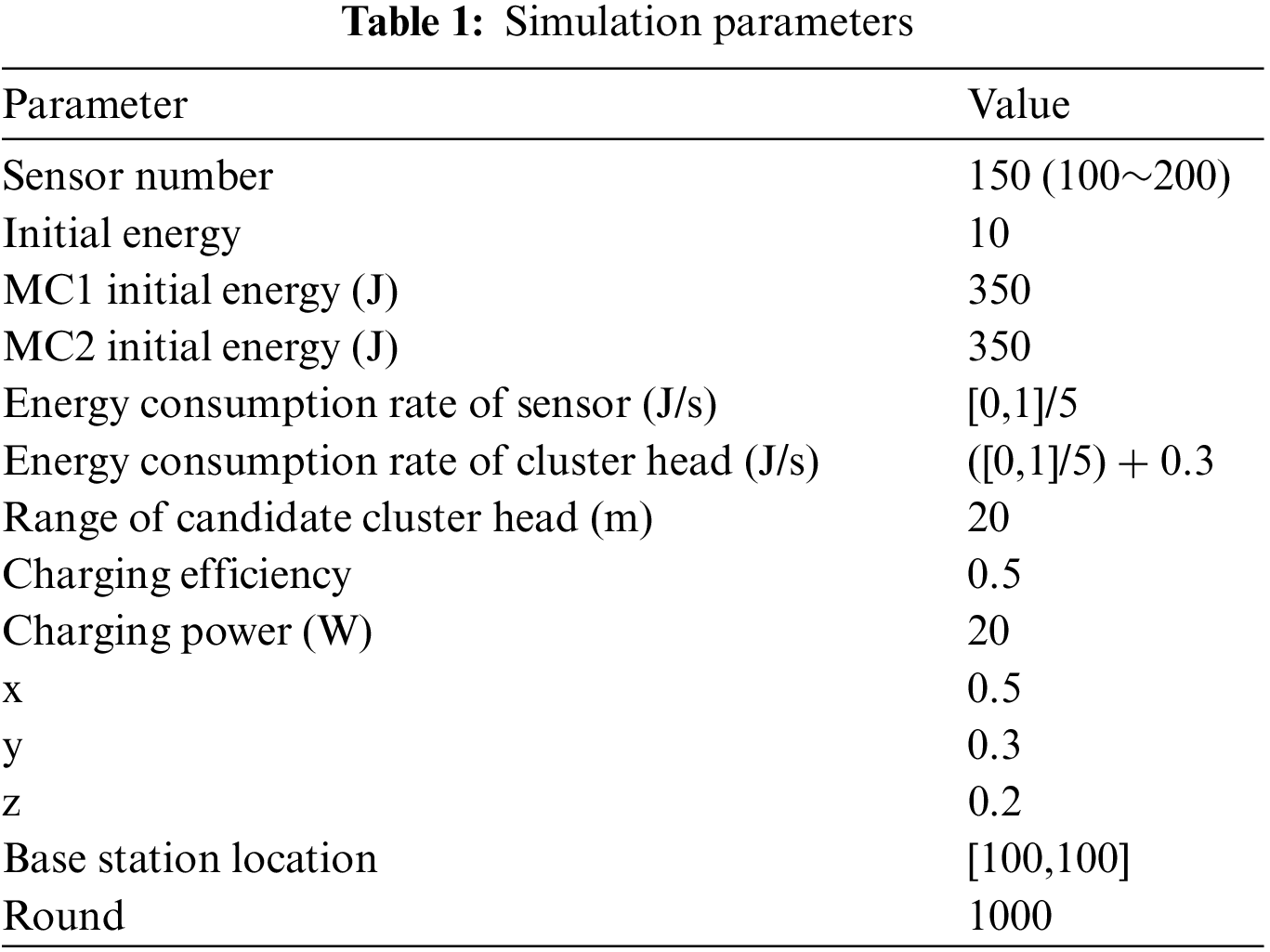
This section conducts a simulation analysis of the algorithm proposed in this paper using MATLAB R2018a software. The simulation parameters refer to the research [21]. In the paper, the monitoring area is set as a square area of 200 (m) × 200 (m). The base station is in the center, and the initial positions of the two MCs are next to the base station. Sensors are randomly placed in the monitoring area. The energy consumption rate of sensor nodes is random and varies with time. The simulation parameters are shown in Table 1.

To evaluate the performance of the CCSA scheme proposed in this paper, four indicators of the scheme are used to evaluate the scheme: The number of surviving sensors, the total remaining energy, the mobile energy consumption ratio, and the occurrence time of the first dead node. The following algorithms have been compared: NJNP [9], DBCS [21], DWDP [22] and IOCS [23].

5.1 Comparison of Different Network Sizes

Fig. 2 shows the comparison results of the dead rate among five algorithms under different numbers of sensor nodes in the 1000th round. Regardless of the total number of nodes, our proposed algorithm has a greater number of surviving nodes compared to the other four algorithms. When the number of sensors is small, MC can timely replenish energy for nodes, so the dead ratio is lower at this time. The proportion of dead sensors of IOCS is only 9% lower than that of NJNP in a network size of 100 sensors. In the network scale of 150 sensors, its value rises to a maximum of 19%. As the number of nodes increases, the charging requests from the nodes also increase. CCSA adopts a collaborative charging mode and partially charges member nodes, which can respond to more charging requirements and achieve the lowest dead rate.

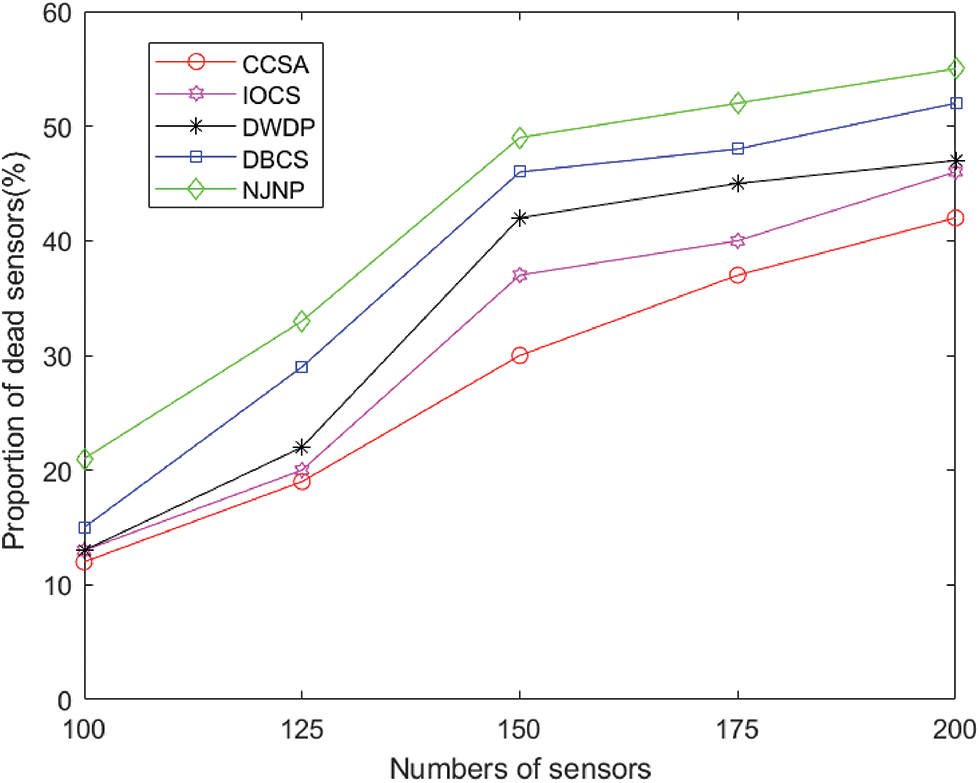
Figure 2: The impact of the number of sensors on the network

5.2 Comparison of the Number of Surviving Sensors

Fig. 3 shows the comparison result of the number of surviving sensors for the five algorithms. Fig. 3 shows that CCSA is followed by DWDP, DBCS, and IOCS, and NJNP has the least surviving sensor nodes. This is because NJNP gives priority to charging the nearest sensor node, which makes some remote sensors unable to obtain energy supplements. DWDP and DBCS choose the charging sensor based on the waiting time of sensor nodes. Compared with DWDP and DBCS, CCSA chooses the charging sensor based on the life and real-time energy consumption of the sensor node, thus can replenish energy for sensor nodes to be charged in time. Compared with IOCS, CCSA can improve the overall survival rate of member sensor nodes by using partial charging. After a period of operation, the network tends to be stable. Compared with the other algorithms, CCSA reaches a stable state after about 200 rounds, while other algorithms tend to stabilize after around 400 rounds. The number of surviving nodes after stabilization is more than the other four algorithms. Compared with IOCS, DWDP, DBCS, and NJNP, CCSA has increased by 11.70%, 20.68%, 29.62%, and 38.15%, respectively.

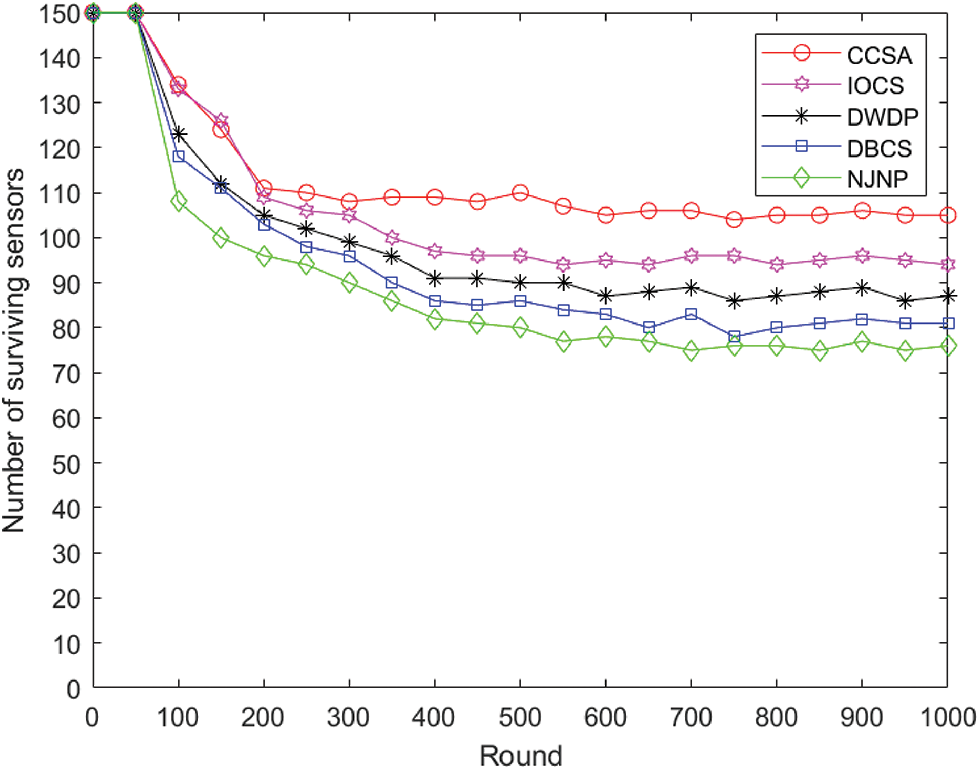
Figure 3: Comparison of the number of surviving sensors

5.3 Comparison of the Total Remaining Energy

Fig. 4 shows the comparison result of the total remaining energy of the five algorithms. As the number of rounds increases, the total remaining energy of the four algorithms decreases continuously because MC starts to work only when the sensor nodes reach the energy threshold. After the network becomes stable, NJNP has more total energy consumption, because MC needs to frequently return to the base station for energy replenishment. Compared with IOCS, DWDP, and DBCS, the dual MC collaborative charging mode in CCSA reduces the hole time during MC energy supplement to a certain extent. Idle MC can assist in charging, effectively reducing the charging task of another MC. Compared with IOCS, DWDP, DBCS, and NJNP, the total residual energy of CCSA after stabilization increased by 5.91%, 6.53%, 9.32%, and 13.26%, respectively.

Figure 4: Comparison of total residual energy

5.4 Comparison of Mobile Energy Loss Ratio

The total energy consumption of MC is divided into charging energy consumption and mobile energy consumption. The mobile energy loss ratio of MC is the proportion of MC’s mobile energy consumption to its total energy consumption. Fig. 5 shows the comparison results of the mobile energy loss ratio of the five algorithms. As the network operates, the number of charging requests gradually increases, and NJNP has poor adaptability because it does not consider the life of sensor nodes. DBCS and DWDP only use a single MC and there is no collaborative charging between the MCs of IOCS, and cannot seek help from another MC when the MC energy is insufficient. They consume more energy during multiple round trips to the base station for energy supplements, which increases the mobile energy consumption rate. Compared with IOCS, DWDP, DBCS, and NJNP, the mobile energy loss ratio of CCSA decreased by 10.00%, 14.28%, 21.73%, and 18.18% in the 500th round, and by 19.05%, 26.08%, 30.76% and 29.16% in the 1000th round. The collaborative charging mode in the CCSA scheme allows MC to seek assistance from another MC when its energy is insufficient, which reduces the energy consumed by MC to some extent, thereby reducing the mobile energy loss rate. This shows that the proposed algorithm has a better performance than other algorithms in controlling the unnecessary energy cost of MC.

Figure 5: Comparison of mobile energy loss ratio

5.5 Comparison of Average Charging Latency

Fig. 6 shows the comparison results of the average charging latency for five algorithms. The average charging delay affects the charging efficiency. The shorter the average charging delay, the shorter the waiting time for other nodes and the less likely they are to die due to energy depletion. Compared to other algorithms, CCSA has the lowest average charging latency and exhibits significant stability in comparison to DWDP, DBCS, and NJNP. Compared with IOCS, DWDP, DBCS, and NJNP, the average charging latency of CCSA decreased by 25.00%, 28.00%, 30.77% and 70.37% in the 600th round, and by 21.05%, 31.81%, 37.50% and 50.00% in the 1000th round. During network operation, an increasing number of sensor nodes will die due to energy depletion as the number of rounds increases. Since MC only charges surviving sensor nodes, the average charging latency will decrease as the number of nodes in the request service pool decreases. However, the cost of this reduction is a significant increase in the network hole rate. CCSA adopts an adaptive charging method, and the charging threshold of nodes also changes according to network conditions, ensuring stable changes in the number of requests in the service pool and timely replenishing energy for sensor nodes, thereby achieving better performance in terms of average charging latency.

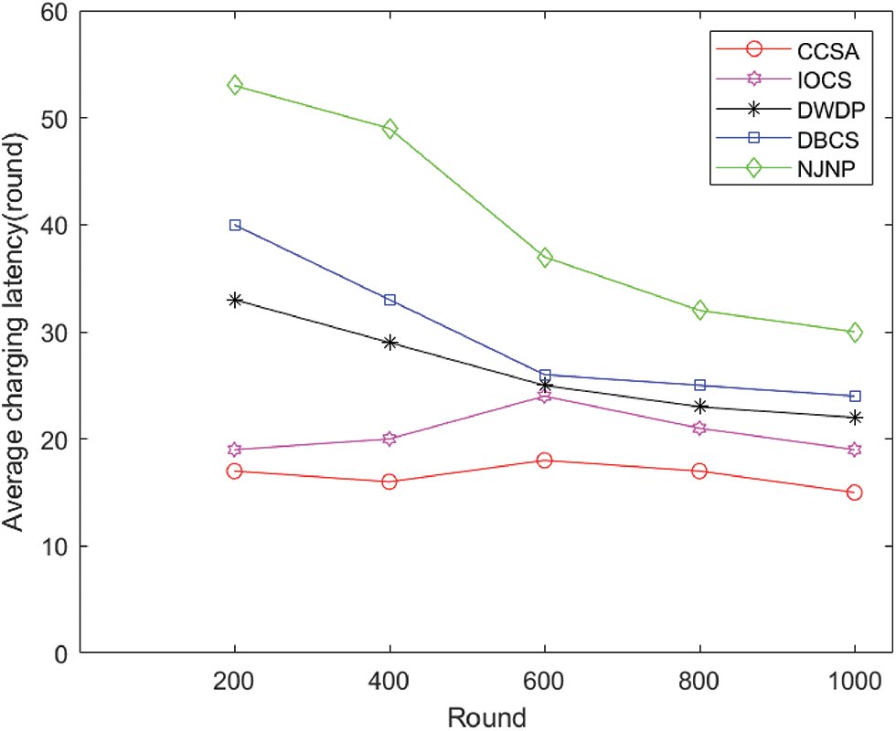
Figure 6: Comparison of average charging latency

5.6 Comparison of the First Dead Sensor

Fig. 7 shows the occurrence time of the first dead sensor for the five algorithms under different sensor numbers. As the number of sensors increases, the number of charging requests increases, and the time of sensor death gradually advances. CCSA adopts a dual MC cooperative charging mode and changes the charging method when the energy of MC2 is insufficient. Under different node numbers, the occurrence of the first dead node in CCSA consistently occurs at the latest. When the number of nodes is small (e.g., 125), CCSA can delay the time of dead nodes by up to 35 rounds, compared to other algorithms. When the number of nodes is large (e.g., 200), the occurrence time of dead nodes appears significantly earlier for each algorithm, however, in CCSA, the occurrence time of dead nodes is delayed by up to 18 rounds, which indicates the success of the proposed algorithm in balancing network energy.

Figure 7: Comparison of the first dead sensor

6  Discussion

We discussed several interesting issues worth studying in the future. For large-scale and complex application scenarios, such as in the Industrial Internet of Things (IIOT) field, sensor nodes usually need to maintain a high-intensity continuous working state, which requires sensor node activity management and joint energy replenishment by multiple MCs. The first problem is how to schedule sensor activation and coordinate multiple MCs to meet the charging deadlines of different sensor nodes. Gao et al. [31] introduced a load-balanced sensor activation scheme and adjusted the energy request time; Shu et al. [36] studied the joint optimization problem of sensor activation/sleep mechanism and charging scheduling. However, it does not apply to the perception scenario of the industrial Internet of Things, and it is necessary to consider using reinforcement learning to assist in optimizing sensor activation, data collection, and charging scheduling. Based on the problem, Lyu et al. [37] proposed a discrete fireworks Q-learning algorithm to solve the multi-WCE charging scheduling problem. Chen et al. [38] proposed a scheme that combines reinforcement learning and marginal benefit approximation algorithms. Secondly, the optimal number of MCs remains an unresolved issue. To deploy varying numbers of MCs in the network and analyze their impact on charging scheduling performance. Considering the interdependence between these two issues, it becomes more difficult to address them in the solution. We plan to study these issues in the future.

7  Conclusion

In this paper, we studied the problem of finding a charging scheduling for dual MC in WRSNs with the objective of maximizing the number of surviving sensors. To solve the problem, this paper proposes a cooperative charging schedule algorithm based on dual MCs. Dual MCs provide the charging services for important sensors and ordinary sensors respectively, and can work collaboratively. The next charging choice of MC is determined according to the life and distance of the sensors. To improve the charging efficiency, a dynamic charging threshold is proposed. In addition, the charging strategy of the MC and sensors is dynamically adjusted according to the network situation. Finally, we demonstrate the advantages of our proposed schemes by extensive simulations. Simulation results show that the proposed algorithm can achieve good performance in terms of network size, the number of surviving sensors, the total remaining energy, mobile energy consumption ratio, average charging latency, and the occurrence time of the first dead node. Specifically, compared with IOCS, DWDP, DBCS, and NJNP, the number of surviving sensors of CCSA can be increased by 11.70%, 20.68%, 29.62%, and 38.15%, and the mobile energy loss ratio of CCSA can be decreased by 19.05%, 26.08%, 30.76%, and 29.16%, respectively.

Acknowledgement: The authors would like to express their gratitude to Professor Dr. Xu Zhen and Professor Dr. Yang Lei for supervising of this study.

Funding Statement: This work is supported by Hubei Provincial Natural Science Foundation of China under Grant No. 2017CKB893 and Wuhan Polytechnic University Reform Subsidy Project Grant No. 03220153.

Author Contributions: The authors confirm contribution to the paper as follows: writing original draft: Qiuyang Wang; project administration: Zhen Xu; data collection: Qiuyang Wang; analysis of results: Lei Yang.

Availability of Data and Materials: The data and materials used to support the findings of this study are available from the corresponding author upon request.

Conflicts of Interest: The authors declare that they have no conflicts of interest to report regarding the present study.

References

1. W. Chen and X. Z. Wang, “Coal mine safety intelligent monitoring based on wireless sensor network,” IEEE Sens. J., vol. 21, no. 22, pp. 25465–25471, 2020. doi: 10.1109/JSEN.2020.3046287. [Google Scholar] [CrossRef]

2. H. Yetgin, K. T. K. Cheung, and M. El-Hajjar, “A survey of network lifetime maximization techniques in wireless sensor networks,” IEEE Commun. Surv. Tutorials, vol. 19, no. 2, pp. 828–854, 2017. doi: 10.1109/COMST.2017.2650979. [Google Scholar] [CrossRef]

3. D. Yan, P. Liu, X. Yue, P. Wang, M. Liu and B. Li, “Data fusion algorithm based on classification adaptive estimation weighted fusion in WSN,” Wirel. Pers. Commun., vol. 127, no. 4, pp. 2859–2871, 2022. doi: 10.1007/s11277-022-09900-x. [Google Scholar] [CrossRef]

4. R. Singh and A. K. Verma, “Energy efficient cross layer based adaptive threshold routing protocol for WSN,” AEU-Int. J. Electron. Commun., vol. 72, pp. 166–173, 2017. doi: 10.1016/j.aeue.2016.12.001. [Google Scholar] [CrossRef]

5. H. S. Cha, S. W. Yoo, T. Lee, J. Park, and K. H. Kim, “An entropy-based clustering algorithm for load balancing in WSN,” Int. J. Sens. Netw., vol. 22, no. 3, pp. 188–196, 2016. doi: 10.1504/IJSNET.2016.080203. [Google Scholar] [CrossRef]

6. G. J. Horng and H. T. Wu, “The adaptive path selection mechanism for solar-powered wireless sensor networks,” Wirel. Pers. Commun., vol. 81, pp. 1289–1301, 2015. doi: 10.1007/s11277-014-2184-2. [Google Scholar] [CrossRef]

7. J. Qiu, H. Chen, Y. Wen, and P. Li, “Magnetoelectric and electromagnetic composite vibration energy harvester for wireless sensor networks,” J. Appl. Phys., vol. 117, no. 17, pp. 092902, 2015. doi: 10.1063/1.4918688. [Google Scholar] [CrossRef]

8. J. H. Cho, B. H. Lee, and Y. J. Kim, “Overview of research status and application of wireless power transmission technology,” Trans. China Electr. Soc., vol. 34, no. 7, pp. 1353–1380, 2019. [Google Scholar]

9. L. He, L. H. Kong, Y. Gu, J. Pan, and T. Zhu, “Evaluating the on-demand mobile charging in wireless sensor networks,” IEEE Trans. Mob. Comput., vol. 14, no. 9, pp. 1861–1875, 2014. doi: 10.1109/TMC.2014.2368557. [Google Scholar] [CrossRef]

10. L. He et al., “Evaluating on-demand data collection with mobile elements in wireless sensor networks,” in 2010 IEEE 72nd Veh. Technol. Conf.-Fall, Ottawa, ON, Canada, Sep. 6–9, 2010, pp. 1–5. [Google Scholar]

11. J. Q. Zhu, Y. Feng, M. Liu, G. Chen, and Y. Huang, “Adaptive online mobile charging for node failure avoidance in wireless rechargeable sensor networks,” Comput. Commun., vol. 126, pp. 28–37, 2018. doi: 10.1016/j.comcom.2018.05.002. [Google Scholar] [CrossRef]

12. C. Lin, Z. Wang, D. Han, Y. Wu, C. W. Yu and G. Wu, “TADP: Enabling temporal and distantial priority scheduling for on-demand charging architecture in wireless rechargeable sensor networks,” J. Syst. Archit., vol. 70, pp. 26–38, 2016. doi: 10.1016/j.sysarc.2016.04.005. [Google Scholar] [CrossRef]

13. Z. S. Chen, H. Shen, T. Wang, and X. Zhao, “An adaptive on-demand charging scheme for rechargeable wireless sensor networks,” Concurr. Comput.: Pract. Exp., vol. 34, no. 2, pp. e6136, 2022. doi: 10.1002/cpe.6136. [Google Scholar] [CrossRef]

14. X. G. Ye and W. F. Liang, “Charging utility maximization in wireless rechargeable sensor networks,” Wirel. Netw., vol. 23, no. 7, pp. 2069–2081, 2017. doi: 10.1007/s11276-016-1271-6. [Google Scholar] [CrossRef]

15. L. G. Xie, Y. Shi, Y. T. Hou, and H. D. Sherali, “Making sensor networks immortal: An energy-renewal approach with wireless power transfer,” IEEE/ACM Trans. Netw., vol. 20, no. 6, pp. 1748–1761, 2012. doi: 10.1109/TNET.2012.2185831. [Google Scholar] [CrossRef]

16. P. Guo, X. Liu, S. Tang, and J. Cao, “Concurrently wireless charging sensor networks with efficient scheduling,” IEEE Trans. Mob. Comput., vol. 16, no. 9, pp. 2450–2463, 2016. doi: 10.1109/TMC.2016.2624731. [Google Scholar] [CrossRef]

17. T. S. Chen, J. J. Chen, and X. Y. Gao, “Mobile charging strategy for wireless rechargeable sensor networks,” Sensors, vol. 22, no. 1, pp. 359, 2022. doi: 10.3390/s22010359 [Google Scholar] [PubMed] [CrossRef]

18. T. Li, T. Liu, J. Peng, F. Lin, and W. Xu, “Charge critical sensors first: Minimize data loss in wireless rechargeable sensor networks,” Int. J. Distrib. Sens. Netw., vol. 14, no. 7, 2018. doi: 10.1177/1550147718784479. [Google Scholar] [CrossRef]

19. T. Shan, Y. Wang, C. Zhao, Y. Li, G. Zhang and Q. Zhu, “Multi-UAV WRSN charging path planning based on improved heed and IA-DRL,” Comput. Commun., vol. 203, no. 1, pp. 77–88, 2023. doi: 10.1016/j.comcom.2023.02.021. [Google Scholar] [CrossRef]

20. S. Soni and M. Shrivastava, “Novel wireless charging algorithms to charge mobile wireless sensor network by using reinforcement learning,” SN Appl. Sci., vol. 1, pp. 1–18, 2019. doi: 10.1007/s42452-019-1091-2. [Google Scholar] [CrossRef]

21. Y. Dong, Y. Wang, and S. Li, “Demand-based charging strategy for wireless rechargeable sensor networks,” ETRI J., vol. 41, no. 3, pp. 326–336, 2019. doi: 10.4218/etrij.2018-0126. [Google Scholar] [CrossRef]

22. C. Lin, Y. Sun, K. Wang, Z. Chen, B. Xu and G. Wu, “Double warning thresholds for preemptive charging scheduling in wireless rechargeable sensor networks,” Comput. Netw., vol. 148, pp. 72–87, 2019. doi: 10.1016/j.comnet.2018.10.023. [Google Scholar] [CrossRef]

23. Y. Dong et al., “Instant on-demand charging strategy with multiple chargers in wireless rechargeable sensor networks,” Ad Hoc Netw., vol. 136, pp. 102964, 2022. doi: 10.1016/j.adhoc.2022.102964. [Google Scholar] [CrossRef]

24. L. R. Tang, J. Cai, J. Yan, and Z. Zhou, “Joint energy supply and routing path selection for rechargeable wireless sensor networks,” Sensors, vol. 18, no. 6, pp. 1962, 2018. doi: 10.3390/s18061962 [Google Scholar] [PubMed] [CrossRef]

25. M. Sheikhi, S. Sedighian Kashi, and Z. Samaee, “Energy provisioning in wireless rechargeable sensor networks with limited knowledge,” Wirel. Netw., vol. 25, no. 6, pp. 3531–3544, 2019. doi: 10.1007/s11276-019-01948-1. [Google Scholar] [CrossRef]

26. S. Alkhalidi, D. Wang, and Z. A. A. Al-Marhabi, “Sector-based charging schedule in rechargeable wireless sensor networks,” KSII Trans. Int. Inf. Syst., vol. 11, no. 9, pp. 4301–4319, 2017. [Google Scholar]

27. S. Priyadarshani, A. Tomar, and P. K. Jana, “An efficient partial charging scheme using multiple mobile chargers in wireless rechargeable sensor networks,” Ad Hoc Netw., vol. 113, pp. 4102407, 2021. doi: 10.1016/j.adhoc.2020.102407. [Google Scholar] [CrossRef]

28. K. Wang, L. Wang, and M. S. Obaidat, “Extending network lifetime for wireless rechargeable sensor network systems through partial charge,” IEEE Syst. J., vol. 15, no. 1, pp. 1307–1317, 2020. doi: 10.1109/JSYST.2020.2968628. [Google Scholar] [CrossRef]

29. M. Razzaq, D. D. Ningombam, and S. Shin, “Energy efficient K-means clustering-based routing protocol for WSN using optimal packet size,” in 2018 Int. Conf. Inf. Netw. (ICOIN), Chiang Mai, Thailand, Jan. 10–12, 2018, pp. 632–635. [Google Scholar]

30. G. J. Han, X. Yang, L. Liu, and W. Zhang, “A joint energy replenishment and data collection algorithm in wireless rechargeable sensor networks,” IEEE Internet Things J., vol. 5, no. 4, pp. 2596–2604, 2017. doi: 10.1109/JIOT.2017.2784478. [Google Scholar] [CrossRef]

31. Y. Gao, C. Wang, and Y. Y. Yang, “Joint wireless charging and sensor activity management in wireless rechargeable sensor networks,” in 2015 44th Int. Conf. Parallel Process., Beijing, China, Sep. 1–4, 2015, pp. 789–798. [Google Scholar]

32. P. Zhong, Y. Zhang, S. Ma, X. Kui, and J. Gao, “RCSS: A real-time on-demand charging scheduling scheme for wireless rechargeable sensor networks,” Sensors, vol. 18, no. 5, pp. 1601, 2018. doi: 10.3390/s18051601 [Google Scholar] [PubMed] [CrossRef]

33. M. Q. Tian, W. G. Jiao, and G. Z. Shen, “The charging strategy combining with the node sleep mechanism in the wireless rechargeable sensor network,” IEEE Access, vol. 8, pp. 197817–197827, 2020. doi: 10.1109/ACCESS.2020.3035473. [Google Scholar] [CrossRef]

34. A. O. Almagrabi, “Fair energy division scheme to permanentize the network operation for wireless rechargeable sensor networks,” IEEE Access, vol. 8, pp. 178063–178072, 2020. doi: 10.1109/ACCESS.2020.3027615. [Google Scholar] [CrossRef]

35. J. Yang, J. S. Bai, and Q. Xu, “An online charging scheme for wireless rechargeable sensor networks based on a radical basis function,” Sensors, vol. 20, no. 1, pp. 205, 2019. doi: 10.3390/s20010205 [Google Scholar] [PubMed] [CrossRef]

36. Y. C. Shu, K. G. Shin, J. Chen, and Y. Sun, “Joint energy replenishment and operation scheduling in wireless rechargeable sensor networks,” IEEE Trans. Ind. Inform., vol. 13, no. 1, pp. 125–134, 2016. doi: 10.1109/TII.2016.2586028. [Google Scholar] [CrossRef]

37. Z. W. Lyu, P. Li, Z. Wei, J. Xu, and L. Shi, “A novel mobile charging planning method based on swarm reinforcement learning in wireless sensor networks,” Int. J. Sens. Netw., vol. 41, no. 3, pp. 176–188, 2023. doi: 10.1504/IJSNET.2023.129813. [Google Scholar] [CrossRef]

38. J. Y. Chen et al., “Optimization of data collection and charging in industrial wireless rechargeable sensor,” J. Chinese Comput. Syst., vol. 72, no. 4, pp. 5064–5078, 2023. [Google Scholar]