Spinal Vertebral Fracture Detection and Fracture Level Assessment Based on Deep Learning

1  Introduction

Spinal fractures are a common type of fracture, with vertebral fractures being the most frequent. Such fractures may be caused by pathologic, traumatic, or nontraumatic causes [1]. This systemic skeletal disorder has serious implications for the elderly and chronically ill [2]. Globally, it is estimated that approximately 1.4 million new clinical vertebral fractures occur each year. Their CT (Computed Tomography) image reading is a huge workload and time-consuming. It also results in significant medical and social costs. Often, vertebral fractures may go undetected due to a variety of reasons, such as the asymptomatic nature of the fracture in its early stages, the failure of radiologists to detect the fracture in time due to inadvertence, and the difficulty in distinguishing between normal and pathologically deformed vertebrae because of the extreme similarity in their shapes. If omission or misdiagnosis occurs or patients are not treated in time, these vertebral fractures may lead to secondary fractures, causing permanent disability or even death [3]. Therefore, early detection of vertebral fractures is extremely important for the prevention of secondary fractures.

In this context, some researchers have proposed methods for intelligent diagnosis of vertebral fractures, and most of the initial studies have focused on machine learning. Valentinitsch et al.’s study [4] employed a random forest (RF) classifier to identify vertebral compression fracture (VCF) based on texture features and regional vertebral bone mineral density (BMD) analysis and experimented with more than 200 patients with good results. Wang et al. [5] used a set of support vector machines (SVMs) to classify fractures and considered different sets of features, including measurement features, longitudinal features, and combinations of both. Burns et al. [6] used a water-shed algorithm to segment the vertebrae. And then extracted the vertebral heights and bone density. These features were used to train a support vector machine to grade compression fractures. It achieved a sensitivity of 95.7% and a false positive rate of 0.29.

Recently, deep learning has been used for automatic vertebral fracture detection in medical images [7,8]. Murata and other scholars [9] proposed a spinal fracture detection method based on a deep convolutional neural network (DCNN). It was trained using plain thoracolumbar radiography (PTLR) images of 300 patients (150 patients with VF and 150 patients without VF). The resultant accuracy, sensitivity, and specificity were 86.0%, 84.7%, and 87.3%, respectively. Bar et al. [10] first segmented the spine portion of a computed tomography (CT) scan and divided it into two-dimensional sagittal section slices. Then, the sagittal slices were classified using a (2D) CNN. Similarly. Tomita et al. [11] proposed a 2D CNN-based recognition method that first abstracts data from CT slices using a CNN feature extraction module. and then determines vertebral fractures using a Long Short-Term Memory (LSTM) network-based approach. Although these 2D CNN-based methods can judge vertebral fractures more effectively, their limitation is that they cannot fully utilize the information of the complete vertebral sequence, which may easily result in missing information.

A full 3D convolution-based approach can be effective in solving this problem. Nicolaes et al. [12] proposed a two-stage VCF detection method by firstly cropping the vertebral body using the vertebral body center of mass co-ordinates labeled by a physician and then 3D CNN predicting the category probability for each voxel (fractures and non-fractures). This study demonstrated the advantages of 3D CNN, but its main drawback was that only a small dataset containing 90 patients was used, and that the method was a semi-automated diagnostic approach. Chettrit et al. [13] proposed an end-to-end 3D CNN-based architecture for vertebral fracture detection, whereby the framework inputs axial CT images of the thorax and abdomen and 3D reconstructs a 3D model of the entire spine, which is used to locate the vertebral body. The YOLO detector was then used to localize the location of the vertebrae in each slice, and these slices were filtered and clipped based on the localization results. Finally, these combined slices are used to make fracture judgments using a full 3D CNN. Although this method avoids the manual labeling of vertebral body center of mass, the YOLO detector may not be identical in each CT slice, which may lead to errors in vertebral body location clipping, and also cannot distinguish the vertebral body corresponding to each slice, which will have a certain impact on the subsequent fracture judgment.

To address the above problems, this study proposes a fully automated 3D CNN-based intelligent recognition system for vertebral fractures. The difference is that this paper adopts the M-SCN [14] key point regression model for the selection of a vertebral position, which can directly regress the vertebral center of mass position on the 3D structure without the need to be processed on each slice, and subsequently determine the vertebral type through multi-label segmentation, which adopts the segmentation in with the fracture degree of each vertebra can be evaluated.

The innovations of this article are summarised as follows:

1. In this paper, an M-SCN network is used to automatically locate the center of mass coordinates of each vertebra without the need for physicians to manually label vertebral center of mass coordinates or analyze individual slices. The category name of the current vertebra is then determined based on the location of the feature map where the heatmap is located.

2. Based on the localization results, local vertebrae are centrally cropped to eliminate a large amount of redundant information and to make the current vertebrae located in the centerof the image, so that the vertebral body information in the image is more explicit. This cropped region is then segmented into individual vertebrae using the U-Net [15] network, and the result is divided into background voxels, fractured vertebrae and normal vertebrae.

3. Based on the segmentation results of individual vertebrae, a smart fracture-level assessment method was introduced. The sagittal 2D slices required for Genant assessment were selected using the vertebral bone center as a benchmark, and the key points of vertebral bone morphology were regressed again using the M-SCN network structure, and the final assessment results were obtained according to the Genant formula.

4. This paper improves and optimizes the SCN network. In the LN stage, this study introduces the Attention mechanism and the U-Net network structure, and incorporates residual connections in the convolution block to improve the model robustness and network output accuracy. In the GN stage, this paper adds a multiple filtering design, and takes the 4-layer feature map output from the decoder in the LN stage and the LN output heatmap as the input to the GN. By re-extracting the features of the LN heatmap, each layer of the feature map of the LN decoder is filtered separately using dot product, and finally the GN output heatmap is obtained by up-sampling and re-convolution.

In conclusion, the system proposed in this study can be used in clinical practice. It allows early detection of patients with suspected vertebral fractures. Targeted therapeutic measures can be performed, thus reducing the burden of fracture diagnosis on a wider scale.

2  Method

2.1 Method Overview

As shown in Fig. 1, the method proposed in this paper is divided into two steps: In the first step, the vertebral body center of mass is localized by M-SCN network, and in the second step, the surrounding voxels were clipped according to the vertebral center-of-mass coordinates, and the clipped vertebrae were segmented with multiple labels using the U-Net model (divided into three label masks: Background, fracture, and normal, respectively). Subsequently, the morphological key points required for vertebral fracture grade assessment were regressed using the same network structure as in step one. Then the assessment results were obtained according to the Ganent Semi-Qualitative Assessment [16] formula.

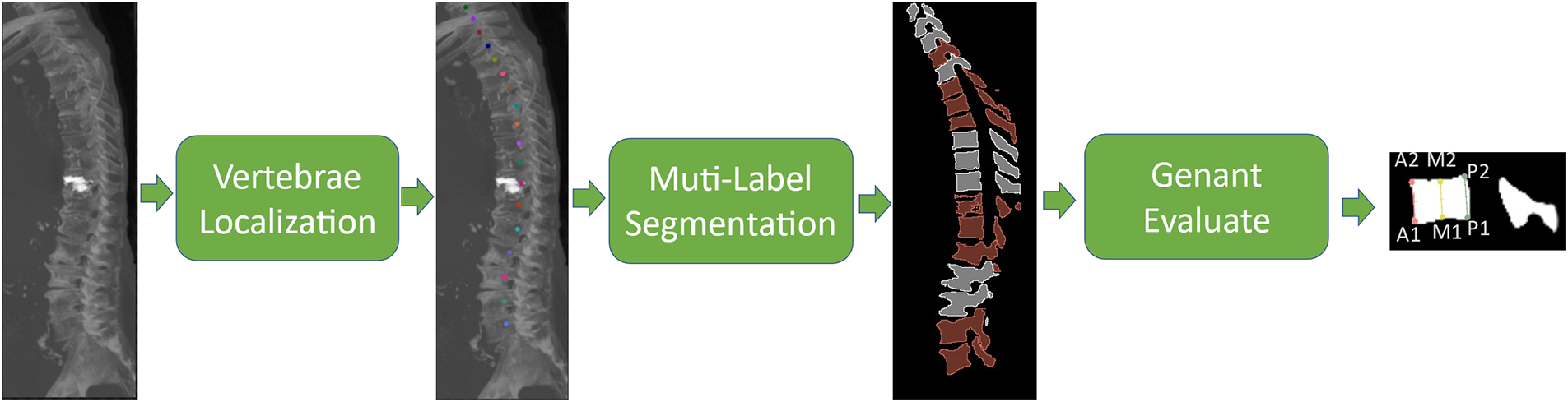
Figure 1: Vertebral fracture analysis process. Firstly, the vertebral center of mass in the original CT image was localized, followed by multi-label image segmentation, and the segmented vertebral fractures were evaluated according to the Genant principle

In Step 1, the entire M-SCN network framework process starts with the input CT image to be detected, which is first sampled to a uniform 1mm voxel interval. The Overlapping approach is adopted, as shown in Fig. 2 (patch size is 96, 96, 128), which demonstrates the heatmap regression results using the M-SCN network model to reason about the whole CT image. Subsequently, the coordinate information represented by the current heatmap was filtered based on the highest brightness in the center of the heatmap.

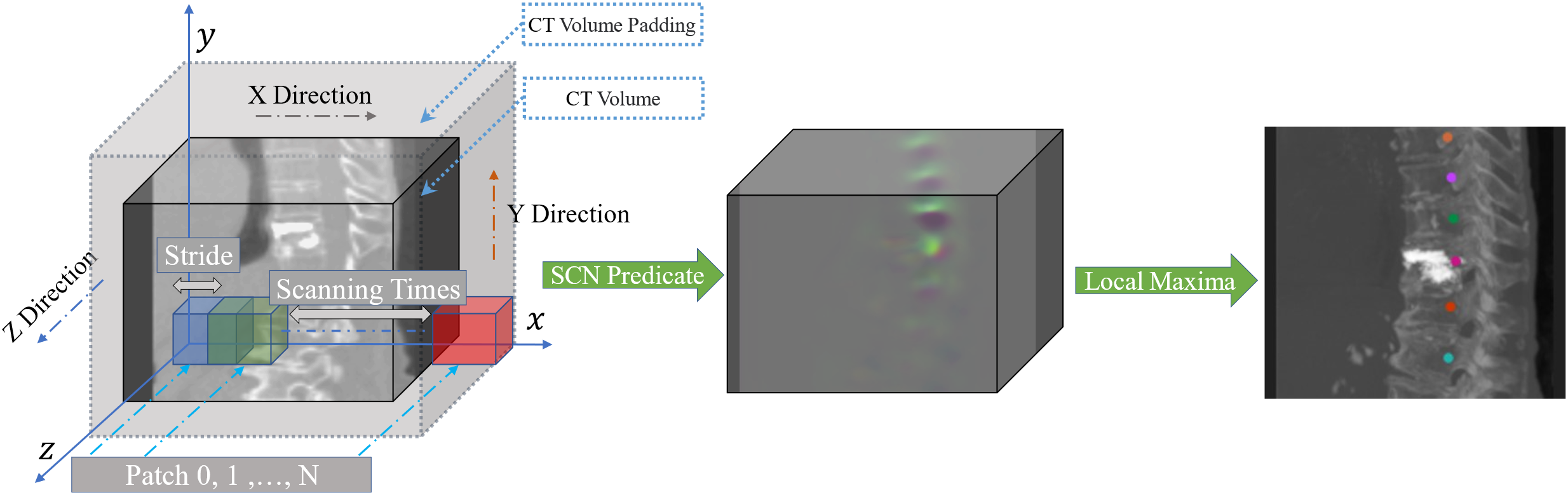
Figure 2: Overlapping patch inference. The original CT image is first filled to ensure that the original CT image is scanned in its entirety. The squares in the figure represent the selected patches, which are scanned along the xyz direction of the whole CT image. The blue squares represent the location of the first patch, the green squares represent the location of the second patch with stride as the offset, and the red squares represent the last patch scanned in the current x-direction. the process is repeated until the entire CT image is scanned, and the entire predicted heatmap is obtained and the coordinates are filtered out

Step 2 is shown in Fig. 3, based on the coordinate information regressed by the localization network, the surrounding voxels (patch size 128, 128, 128) centered on this coordinate are cropped to remove some redundant information and to make the vertebrae represented by the current point located in the center of the cropped image. Use the model U-Net to reason about the multi-label segmentation results, classified into three labels: Background, normal vertebrae, and fractured vertebrae. And retaining the current Patch inference result, it is also necessary to resample the cropped Patch positions to the positions in the original CT image and combine them. This process is repeated until all coordinate traversals are finished.

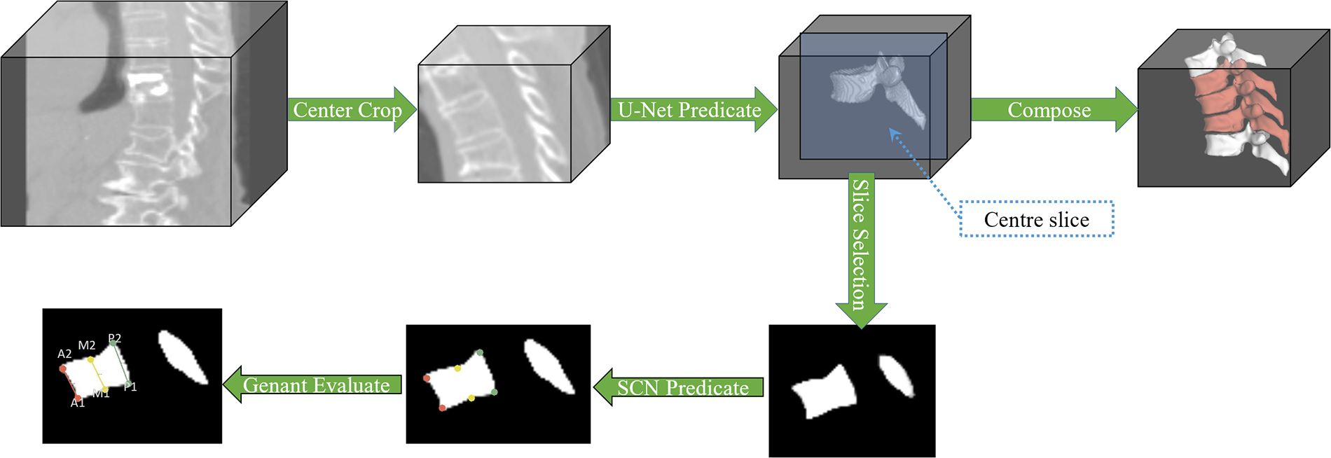
Figure 3: Segmentation and vertebral Genant evaluation process. Firstly, individual vertebrae were centrally clipped, the current vertebrae were segmented by U-Net, the current predicted patch was retained, and the patch was resampled and combined to obtain the whole spine segmentation image. Secondly, the center of the patch was selected and sliced for Genant semi-qualitative assessment

In the vertebral fracture grade assessment stage, as shown in Fig. 3, the Patch segmentation result obtained during the segmentation process was first adjusted to a binary mask. Secondly, the sagittal plane slice at the center of this segmented image was selected as the assessment object. Since it is difficult to obtain the coordinates of the points to be assessed by traditional methods, a fixed-point strategy similar to that of Step 1 is used to regress the required vertebral morphology coordinate points in the 2D dimension. Then the HA, HM, and HP vertebral bone morphology parameters were calculated to obtain the assessment results according to the Ganent semi-qualitative assessment formula.

2.2 Vertebrae Localization

In this paper, the M-CSN network is used to localize the vertebral centers. Which is modeled by two parts, the LN and the GN. In this two-part structure, the role of its GN is to filter and noise-reduce the output of the LN to make the network output more accurate. The major difference between these two networks is the size of the receptive field [17], the LN is designed to extract local features that are mostly valid but can be noisy for the target heatmap, And the GN is designed as a network structure with a large convolutional kernel for extracting the global features. which has a larger receptive field and filters the output of the LN. Fig. 4 shows the vertebral localization network. Since the M-SCN model output is a target heatmap, no activation function is used in the last layer of the model [18]. Where LN convolution block and GN convolution block are designed as shown in Fig. 5.

Figure 4: M-SCN network structure, the model consists of two parts, the local network and the global network. The local network is a U-shaped structure with an attention mechanism. The global network is a U-shaped structure containing a large convolutional kernel, which is mainly used for feature filtering. This network inputs the features of each layer of the LN decoder as well as the LN heatmap. The LN heatmap is re-featured and dot-multiplied with the output of each layer of the decoder, and finally the GN heatmap is obtained by up-sampling and re-convolution. The final output of the model is the result of dot product of LN heatmap and GN heatmap

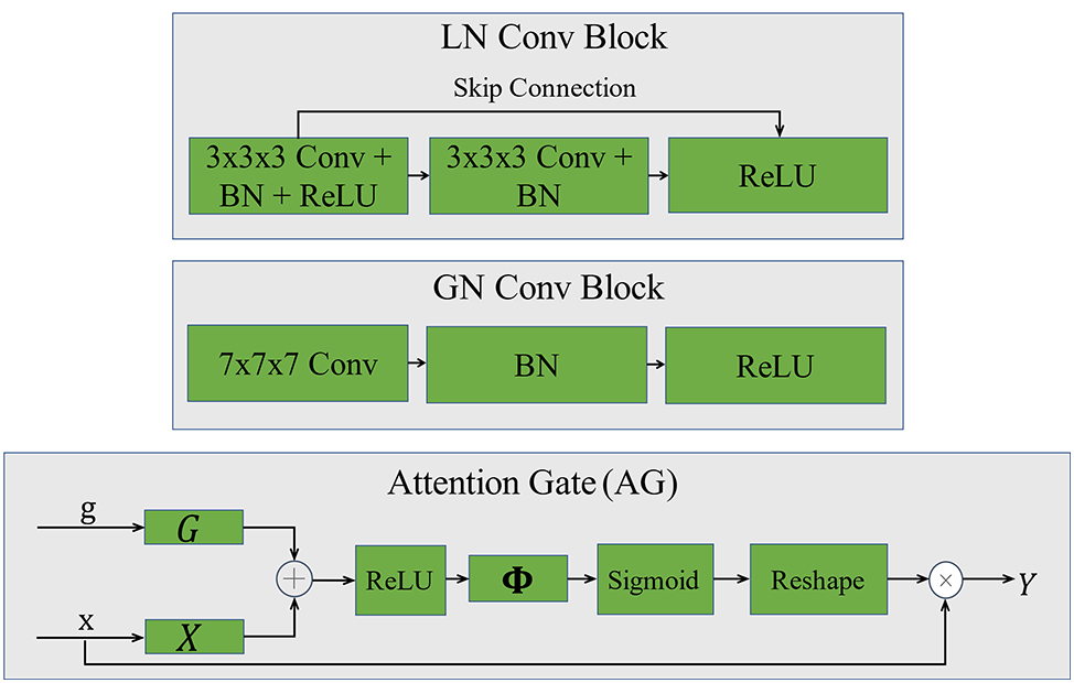
Figure 5: Convolutional block and attention mechanism. LN convolutional block is designed with double-layer convolution and residual joins are added. GN convolutional block is designed with single-layer convolution, which reduces the amount of model computation. Also 7 × 7 × 7 large convolution kernel is used instead of small convolution kernel

Assuming that the input image is Xi∈RCi×Zi×Hi×Wi and its corresponding vertebral center of mass coordinates are lgt={(xic ′,yic ′,zic ′)}, and the labeled heatmap Yik∈RCi ′×Zi×Hi×Wi for the kth(k∈[1,2,⋯,Ci]) image by using a Gaussian distribution function:

Yik=g(xi,σi)=12πσiexp⁡(−(x−lgt)22σi2)(1)

As a result, thermal pixels with target coordinates near lgt will have higher values, and these values will decrease smoothly but quickly as they move away from lgt. The standard deviation σi is used to determine the peak width of the Gaussian function in the thermogram image. where is the number of channels on the input image (for CT images, Ci = 1), Ci ′ is the number of channels on the output thermogram (representing the number of vertebrae), Zi is the value of the image Xi along the cross-section. Hi is the value of the image Xi along the coronal plane. Wi is the value of the image Xi along the sagittal plane.

Similarly, coordinate positions can be determined by obtaining the maximum value in the heatmap.

lcoord=argmax(gi(x;σi))(2)

The M-SCN network regresses the heatmaps of N target vertebrae by minimizing the Euclidean distance between the predicted and labeled heatmaps so that the predicted values gradually approximate the true values, which can be described as:

L=minw,b∑i=1N∑x‖hi(x;w,b)−gi(x;σi‖22+λ‖w‖22(3)

where w is the network weight, b is the network bias, and λ controls the effect of the L2 paradigm of the network weight w.

2.2.1 Local Network

The purpose of LN is to extract local features and generate local heatmaps. In this paper, U-shaped structure with Attention Gates (AG) mechanism is used as the LN structure and residual connectivity is added to the LN convolutional block to improve the robustness of the model. The AG (Attention Gates) module [19] automatically learns and distinguishes the shape of the target and automatically recognizes the region of interest, suppresses irrelevant regions and focuses on features in useful regions. AG can be described as:

f(xi)=WgTxi(4)

attn(xi,gi)=σ1(σ2(f(xi)+f(gi)+b1)+b2)(5)

where the function f(xi) denotes the linear embedding of xi, σ1 denotes the ReLU activation function, and σ2 denotes the Sigmoid activation function. The LN model extracts features from Xi to generate a local heatmap F⌢iL:

F^iL(xi)=hi(xi;wattnL,battn;wsL,bs)(6)

where WattnL is the weight parameter corresponding to the AG module, wsL is the parameter corresponding to the ordinary convolution, battn and bs represent the bias parameters of AG and normal convolution.

2.2.2 Global Network

The GN aims to filter the output features of the LN. Its structure differs in the use of a large 7 × 7 × 7 convolution kernel to extract the features, which provides a larger sensory field for this network, facilitates the capture of important global information [20] and reduces the computational effort by using a single layer of convolution. The inputs to this network are the output heatmap of the LN network and the 4-layer decoded feature map output by the LN decoder, and these 4 layers of decoded features are filtered separately.

F^iG(xi)=hi(F^iL,EiL;wsL,bs)(7)

Finally, the LN heatmap and the GN heatmap are dot-multiplied to obtain the predicted heatmap.

F^i=F^iL⋅F^iG(8)

2.2.3 Loss Function

In this regression task, this paper choose smooth L1 [21] as the loss function, which can be seen from the smooth L1 formula, the gradient is constant when x is a large value, solving the problem of large gradient destroying the training parameters in L2 loss, and when x is a small value, the gradient will be dynamically reduced solving the problem of difficult convergence in L1 loss. It can be defined as:

Smooth−L1(pr,yr)={0.5(σx)2,|x|<1σ2|x|−0.5σ2,otherwise(9)

where pr and yr are the predicted and true values, σ is the smoothing factor. In the experiment, it was set to 1.0.

2.3 Vertebrae Fracture Recognition and Genant Semi-Qualitative Assessment

2.3.1 Identification of Vertebral Fractures

In order to be able to recognize the pathological features of the vertebrae, this paper uses an image segmentation method. The center-of-mass coordinates of each vertebra have been predicted in Task 1 (Vertebral Localization), so the region of interest can be cropped according to the center-of-mass coordinates so that the vertebrae are located in the center of the cropped image, ensuring that the network will only process the current vertebrae. Based on the localization results from Task 1, this process is repeated from top to bottom across the spine until the last vertebra is iterated.

In this paper, U-Net is chosen as the segmentation model, and the prediction results are divided into three state labels, which are background, fractured vertebrae and normal vertebrae. The overall process of vertebral fracture detection is shown in Fig. 6 below.

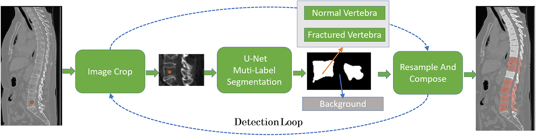
Figure 6: The overall process of vertebral fracture recognition, using U-Net as the segmentation model, based on the vertebral body center of mass predicted in Task 1, clipping the ROI region and performing multi-label task segmentation, which is divided into fracture, normal, and background, and repeating this process until the end of vertebral. Finally, the vertebral segmentation results are combined to obtain an analysis of the entire spine

Let V={v1,v2,…,vn} be the set of coordinates of all vertebrae in the CT image of the spine. The input image is Xi∈RCi×Zi×Hi×Wi. Then there are:

xi=crop(Xi;vi),vi∈V(10)

F^i=hi(xi;w,b)(11)

where xi denotes the image cropped according to the center of mass coordinates vi. F^i denotes the predicted voxel class results.

Similar to Task 1, the vertebral segmentation network approximates the predicted value to the true value by minimizing the difference between the probability distribution of the predicted outcome and the true probability distribution. This can be described as:

L=minw,b∑i=1N∑x1−2|F^i⋅Yi||F^i|2+|Yi|2+Yilog⁡(F^i)+λ‖w‖22(12)

Finally, to create the final multi-label prediction results, the results of the individual predicted images need to be merged. The cropped vertebrae xi also need to be resampled and transformed to their position in the original input image.

2.3.2 Loss Function

Considering the accuracy of predictive segmentation and the matching accuracy of category distribution, this paper uses a combination of dice loss [22] and cross-entropy loss. It can be a more comprehensive measure of the model’s performance in multi-label segmentation tasks. It can be defined as follows:

Loss(pr,py)=1−2|pr⋅py|+ε|pr|2+|py|2+ε+prlog⁡(py)(13)

where pr and py are the predicted and true values, respectively. ε is the smoothing coefficient, which was set to 10−5 in the experiment.

2.3.3 Genant Semi-Qualitative Assessment

Prior to Genant assessment, the sagittal plane needs to be selected from the vertebral fracture segmentation results. For each vertebral image the sagittal plane where the vertebral body center of mass was located was used as a benchmark for Genant assessment. To obtain the key points of vertebral body morphology required for Genant assessment, two problems were faced in this study:

1. As shown in Fig. 7, the traditional Harris corner point detector, although it can detect Genant’s evaluation of key points, still produces a high number of redundant points, does not accurately obtain the corner coordinates, and is extremely dependent on image quality.

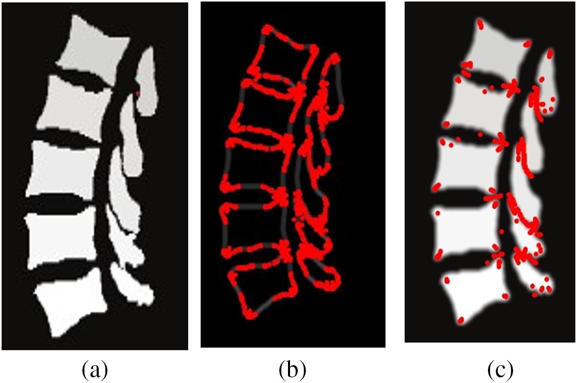
Figure 7: Figure a is the sagittal plane slice, and figure b and c are the Harris corner point detector results after Canny edge detection and smoothing filtering, respectively

2. As shown in Fig. 8, the selection of the M point is more difficult, the M point location does not necessarily contain the corner similar features, so it can not be detected by the Harris corner point detector, if the vertebrae are relatively smooth, the coordinates of the M point can be the average value of the points A, P. If the vertebrae number of biconcave-type (or irregularly shaped) fracture, the location of the M point will occur in the y-axis position of the deviation, Yousefi et al. [23] used the strategy of moving the M point up and down to solve this problem, but there is no universal value for the distance of moving M up and down, and the distance of moving is different for different cases of vertebrae. Therefore this method is more limited.

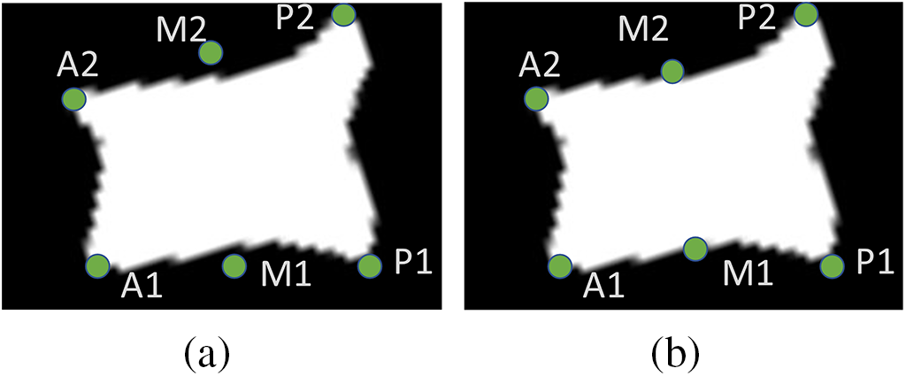
Figure 8: For irregular vertebrae, the selection of M-points produces different degrees of bias among them, figure a is the case when there is a deviation of M point, and figure b is the case when the M point is adjusted by moving up and down

Therefore, this paper uses the same strategy as in Step 1 to regressively localize the desired vertebral morphological keypoints using M-SCN. Fig. 9 shows the overall assessment process.

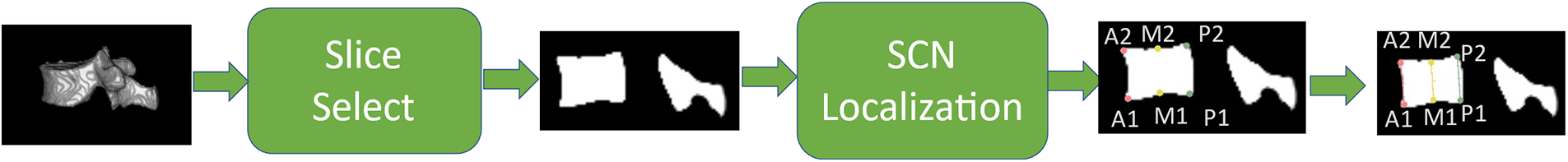
Figure 9: First, the sagittal slice where its center of mass was located was selected based on the segmented vertebrae CT images, and its six points were regressed by M-SCN, and then the Genant value was calculated

It can be described as:

si=Yi[,:ycoord:,](14)

F^i=hi(si;w,b)(15)

lcoord=arg max(F^i)(16)

HP=|P1−P2|,HA=|A1−A2|,HM=|M1−M2|(17)

G=min(HP,HA,HM)max(HP,HA,HM)(18)

where Yi is the input vertebral segmentation mask and si denotes the sagittal slice where the vertebral center of mass is located. lcoord is the key point coordinates, F^i is the predicted heatmap result. HA, HP, HM indicate the morphological heights of the three parts of the vertebrae, Moderately and severely fractured vertebrae (G<0.74), and mildly fractured (0.74<G<0.8) [23].

3  Experiments and Discussions

3.1 Experimental Environment and Dataset

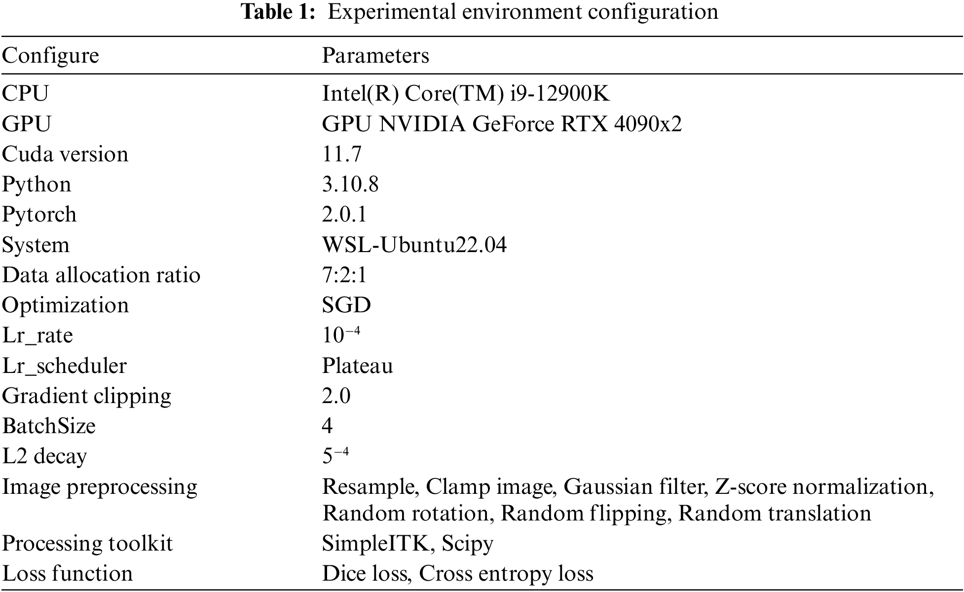
The experimental environment was conducted under the WSL-Ubuntu22.04 system, and the programming environment was python3.10.8, which was completed based on the Pytorch deep learning framework. The relevant hardware environment is CPU Intel(R) Core(TM) i9-12900K, GPU NVIDIA GeForce RTX 4090x2, Cuda version 11.7. 128 GB of RAM and 64-bit operating system.

The dataset used was VerSe’19 and VerSe’20 [24], which is a large dataset of vertebral segmentation and identification organized by MICCAI, where VerSe’19 and VerSe’20 include 160 and 355 CT spine scans, respectively. Spine types included vertebral fractures, metal implants, bone cement, and transitional vertebrae. In this paper, images of vertebral fractures were screened as the training dataset for this study, and 74 CT data provided by Guizhou Orthopedic Hospital were also collected. Fig. 10 a and b shows the vertebral localization data and the vertebral segmentation data, respectively.

Figure 10: Experimental data

3.2 Training Parameter Settings

Raw CT images cannot be used directly for model training. In this paper, SimpleITK is used as a CT data processing toolkit to preprocess and enhance real-time CT data. For each CT image, it was first resampled to a uniform voxel spacing of 1 mm. For each voxel value in the CT volume, it was cropped to between [−2048, 8192] and the overall data was normalized by Eq. (19). Where is the input image, is the image mean, and is the image variance, a very small constant set to 2.220e-16.

x ′=x−μσ2+ε(19)

A total of 30,000 iterations were set for training, the optimizer was SGD, The ratio of training set, validation set and test set was 7:2:1, the learning rate was set to 10−4, the L2 weight regularisation factor was set to 5−4, and the BatchSize was set to 4. In addition, in order to improve the convergence efficiency of the model, gradient clipping was used in the training of the model, and the value of the gradient clipping was set to 2. The details of the experiment are shown in Table 1 below.

3.3 Evaluation of Indicators

In order to evaluate the performance of the network, this paper uses commonly used evaluation methods for studying segmentation [25–27], which can be divided into two categories:

1. The degree of overlap or similarity based on volume. For example, Dice Similarity Coefficient (DSC), Precision, and Recall. Such metrics are used as a way to calculate the similarity between predicted and true values.

2. Measurements based on the distance between the predicted surface and the real surface. For example, maximum symmetric surface distance (MSSD) and average symmetric surface distance (ASSD).

DSC, precision, and recall can be expressed in terms of true positives (TP), false negatives (FN), and false positives (FP). They can be defined as follows:

DSC=2TP2TP+FP+FN(20)

Precision=TPTP+FP(21)

Recall=TPTP+FN(22)

Let’s define the Average Symmetric Surface Distance ASSD, assuming that P is the predicted volume and G is the true volume, as:

ASSD(P,G)=(∑sp∈S(P)d(sp,S(G))+∑sG∈S(G)d(sG,S(P)))|S(P)+S(G)|(23)

where d is the distance metric, and d(sp,S(G)), d(sG,S(P)) are the distances between each point on the predicted surface and the real surface (each point on the real surface and the predicted surface). Where the distance d between the point and the surface can be defined as:

d(lc,S(C))=minlc ′∈S(C)‖lc−lc ′‖(24)

The maximum symmetric surface distance MSSD can be defined as:

MSSD(P,G)=max{h(S(P),S(G)),h(S(G),S(P))}(25)

where h(S(P),S(G)) denotes the one-way Hausdorff distance between the surface of the predicted volume S(P) and the surface of the real volume S(G), defined as follows:

h(S(P),S(G))=supsp∈S(P){infsG∈S(G)d(sp,sG)}(26)

The definition of h(S(G),S(P)) is obtained by the same reasoning.

3.4 Results

3.4.1 Results Overview

A total of 30,000 iterations were set up for this experiment, and the experimental data were recorded every 6,000 iterations due to the long time consumed for each test. Table 2 gives the evaluation results of U-Net vertebral segmentation, it can be seen that the model starts to converge after 12,000 iterations, the maximum value of Dice obtained is 93.50%, the classification performance precision and recall both reach 95.82%, and the recall rate reaches 91.70%, respectively. The ASSD reaches a minimum of 0.262 mm. Fig. 11 shows the model gradient values and network loss values after clipping. In most cases, the model gradient remains between 0 and 1. In contrast using the gradient clipping training method is faster for training and its Loss minimum fluctuates around 0.01. Fig. 12 shows the curve changes of all the indicators, it can be seen that with the increase in the number of training, the model of the various test indicators gradually converge to saturation, and the curve float is small, which also shows that the model prediction output is relatively smooth.

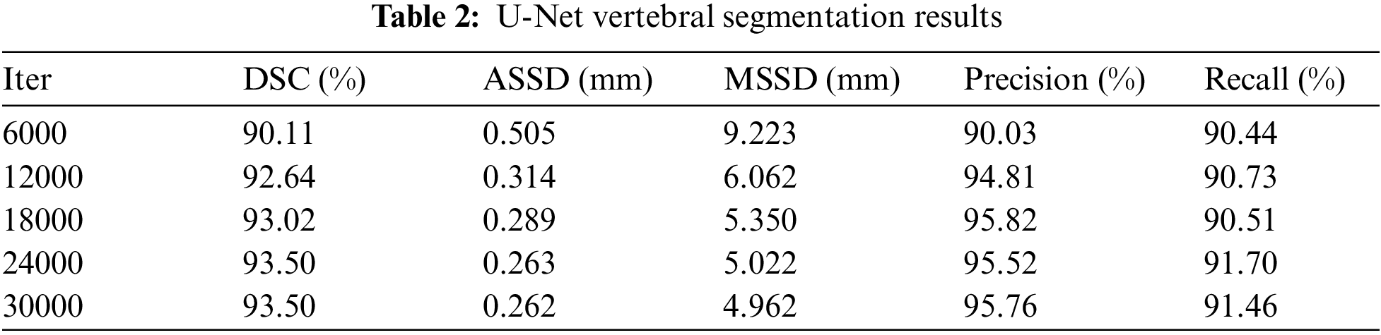
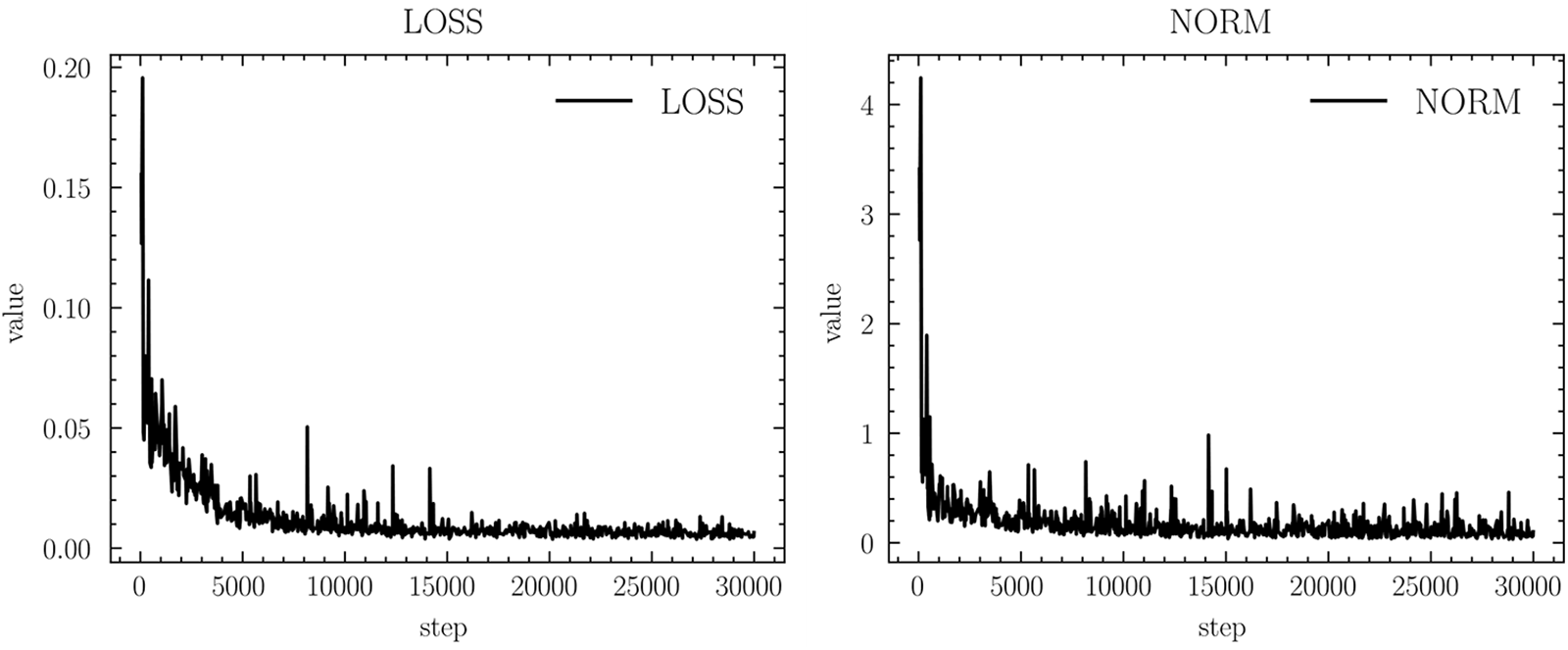
Figure 11: Gradient clipping results in norm and network loss

Figure 12: Segmentation metrics chart

3.4.2 3-Fold Cross Validation

In the current experiments, due to the insufficient number of available datasets, to minimize random results due to a single division of the training and validation sets. Therefore, multiple divisions were performed using the available datasets, thus avoiding the selection of “chance models” that cannot generalize their capabilities due to specific divisions. In this study, the training dataset was divided into three similar subsets, three rounds of cross-validation were performed, and the average of the metrics for the three rounds of training was calculated. The experimental data are shown in Fig. 13, indicating that in the three rounds of cross-validation, the evaluation metrics of the model do not fluctuate much and are relatively smooth, which also indicates that the model has good generalization performance.

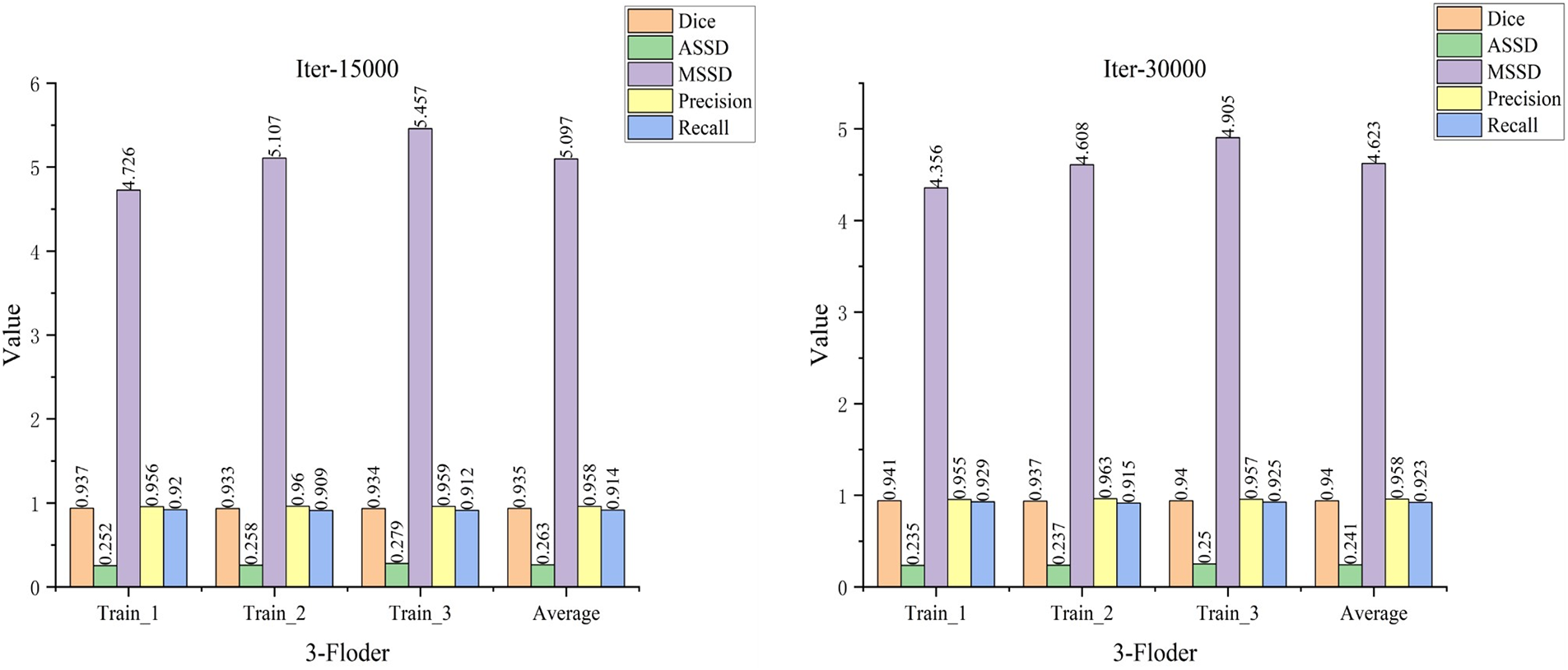
Figure 13: Cross-validation results

3.4.3 Compare with Other Segmentation Models

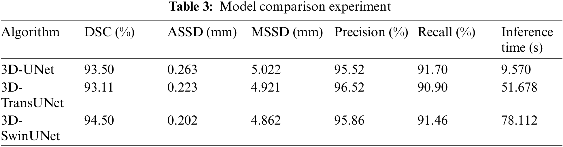
In this paper, a comparison is made with other SOTA models (TransUNet and SwinUNet) and the experimental results are shown in Table 3. In this study, the size of the dataset used is small, and the models that used a Transformer did not have a metric improvement in the evaluation metrics. Whereas the performance of Transformer models usually improves with the size of the model, larger models require more data for training, otherwise they are prone to overfitting. At the same time Transformer also brings a larger amount of computation. In the CT image Overlapping patch inference experiment with size [164, 164, 185], its results show that UNet inference takes 9.570 s, TransUNet takes 51.678 s, and SwinUNet takes 78.112 s. TransUNet and SwinUNet are respectively slower than units by 5.4 times and 8.163 times. Taken together, UNet reasoning is faster and also has higher accuracy, which is more suitable for this task.

3.4.4 M-SCN Network Model Ablation Experiments

In the localization model, an important evaluation metric is the distance between the predicted coordinates and the true coordinates, which is considered to be correctly predicted if the distance is less than 20 mm [28] and can be defined as:

#ID={‖xk−xj ′‖2=PE≤20}(27)

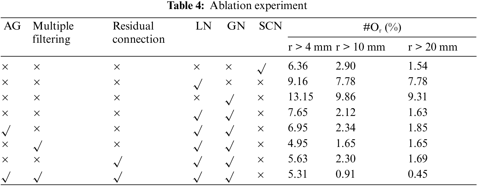
In this paper, the ablation validation of the M-SCN model is carried out to prove the effectiveness of the model improvement. The experimental results are shown in Table 4, where the first column represents the localization results of the SCN model whose prediction error rate is 1.45%. The second and third columns represent the prediction results when only LN or GN is used, and its prediction error rate of 7.78% for LN is better than the prediction error rate of 9.31% for GN, which also highlights that the LN network plays a major role in the localization prediction. The fourth column indicates that LN is used together with GN and its prediction results are close to the SCN network model. Finally in the case of using AG, Multiple Filtering and Residual Connection respectively, their prediction results have been improved accordingly. The last column represents the experimental results of the M-SCN network, which has a prediction error rate of 0.45%, which is 1.09% lower compared to the SCN prediction error rate.

3.5 Visualization and Discussion of Experimental Results

Fig. 14 shows the individual vertebrae segmentation process. In Fig. 14a, the localization results of the M-SCN model are marked using red dots, and Fig. 14b represents the results of cropping the surrounding voxels, whose background and other interfering information have been eliminated. Fig. 14c represents the segmentation result of the current vertebra (the sagittal part of this vertebra is shown), and Fig. 14d represents the result of resampling the position of the vertebra cropped at the current position and restoring it to the initial position. Fig. 14e shows the mixing of the current segmentation result with the original picture.

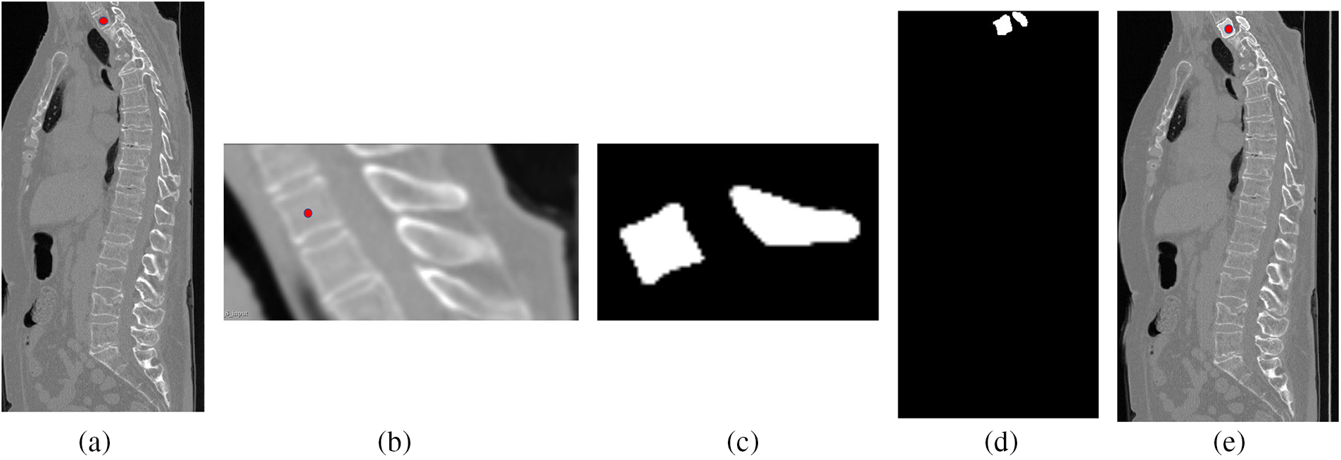
Figure 14: Visualization of the vertebral segmentation process, figure a is the original CT image, figure b is the clipped image, figure c is the result of individual vertebral segmentation, and figure d and figure e are the results of resampling the clipped position to the original position

Fig. 15 shows 2 sets of segmentation results for the entire spine, using white to mark normal vertebrae and red to mark fractured vertebrae. In Fig. 15a, the segmentation results for the L4 and L5 vertebrae show incomplete edge segmentation compared with the actual values, whereas in Fig. 15b, there is redundancy in the segmentation results for the L5 vertebrae. The overall segmentation results meet expectations. From the 3D reconstruction results, it can be seen that the red vertebrae show significant irregularities or depressions compared to the white vertebrae, which also suggests that these vertebrae may have vertebral fractures.

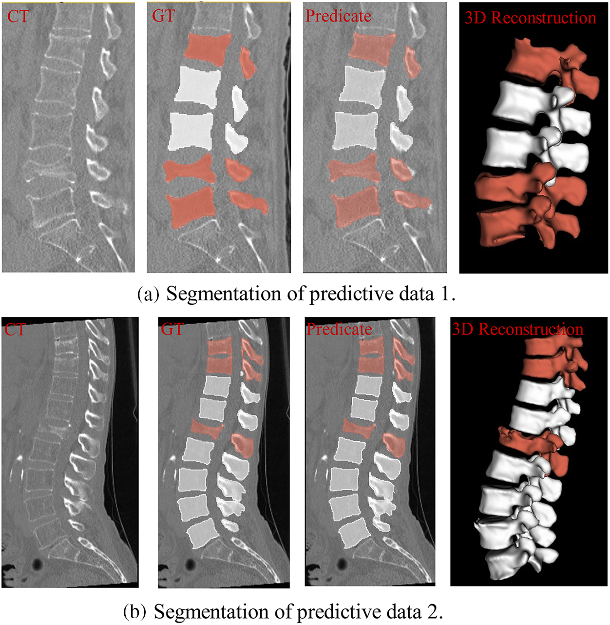
Figure 15: Vertebral segmentation results, where red represents a possible fracture of the vertebral body and white is normal

Fig. 16 illustrates the Genant assessment process. Fig. 16a represents a slice of the original CT image, Fig. 16b represents a sagittal slice of the vertebral body where the center of mass is located, and Fig. 16c represents the results of the Genant assessment. This experiment visualizes the M-SCN prediction heatmap. As shown in Figs. 17, 17a represents the GN output heatmap and Fig. 17b represents the LN output heatmap. Due to the inclusion of 7 × 7 × 7 large convolutional kernel in GN, it has a larger perceptual field than LN, and the final prediction result Fig. 17c also becomes a more prominent data feature due to the filtering effect of GN. Fig. 18 shows the final prediction results of the heatmap after extracting the highlighted areas (maximum values). It can be seen that among the four sets of prediction results, the M-SCN network model’s prediction is more accurate for the middle region, and produces errors for the uppermost and lowermost vertebral marker points. In combination with the segmentation results. This may have contributed to the deterioration of segmentation results in the L4 and L5 vertebrae results.

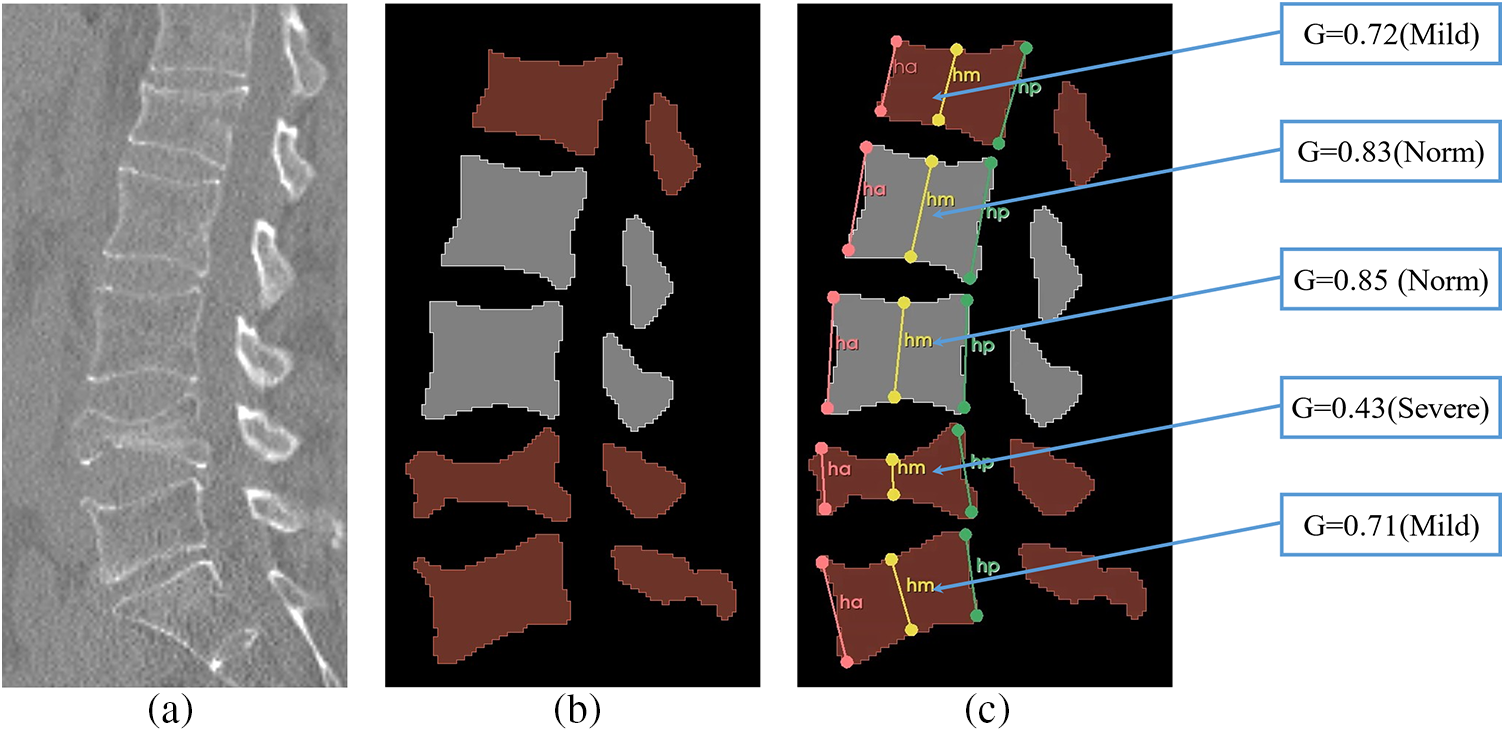
Figure 16: Vertebral Genant semi-qualitative assessment results, a shows the original spinal section image, b shows the segmented image, and c shows the Genant semi-qualitative assessment results

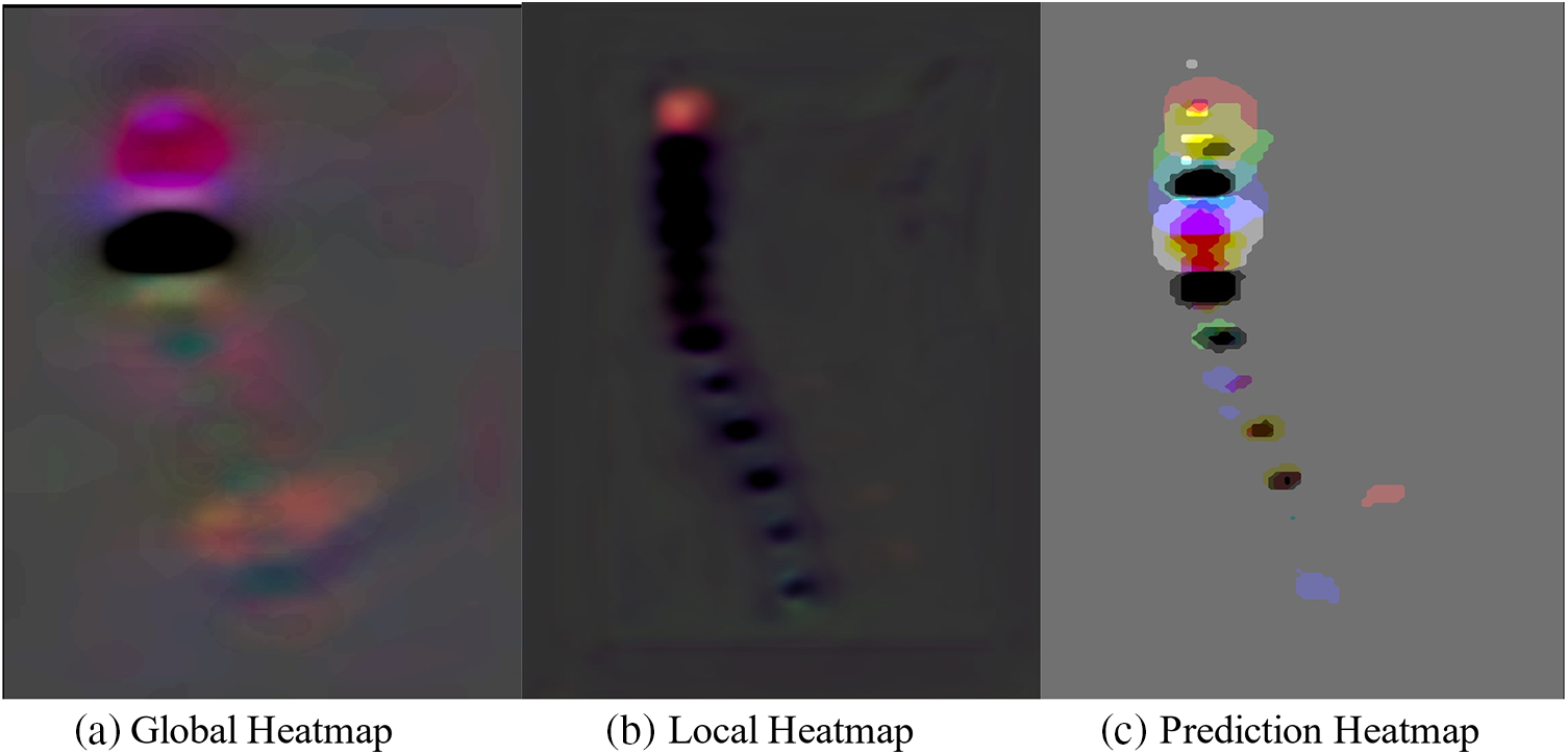
Figure 17: M-SCN prediction heatmap visualization

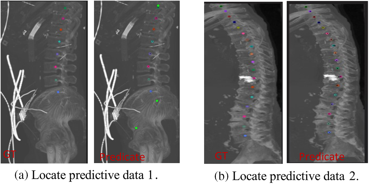
Figure 18: Vertebral localization results

4  Conclusion

This paper describes a fully automated 3D CNN-based system for the intelligent recognition of vertebral fractures. The system performs vertebral fracture detection in two steps (vertebral localization and vertebral segmentation) and subsequently evaluates the fracture grade based on sagittal slices (Genant Semi-Qualitative Assessment).

In this paper, we greatly improved the efficiency and accuracy of vertebral segmentation detection by localizing the vertebrae and clipping the ROI region, and used the segmentation masks obtained from the segmentation model (vertebral fracture mask, normal vertebral mask, and background mask) as the detection results of vertebral fracture. Subsequently, for the segmentation mask, the center sagittal slice was selected according to the center of mass coordinates, the six evaluation key points were regressed by M-SCN, and finally the vertebrae were classified into normal vertebrae and fractured vertebrae (moderate, mild, and severe) according to the Genant semiqualitative assessment. In the experiment, the vertebral segmentation Dice index, ASSD index and MSSD index reached 93.50%, 0.262 and 4.962 mm, respectively, and the vertebral bone localization also achieved relatively excellent results. The comprehensive experimental visualization results show that for some CT images, the localization model and segmentation model still have some defects. In the future, we expect to introduce graph optimization [29] into the keypoint regression model to improve the localization accuracy. And more datasets are collected to improve the accuracy of network training. We expect that the proposed method can effectively improve the diagnostic efficiency of vertebral fracture and can be applied in the clinic.

Acknowledgement: The authors would like to thank the editorial department and reviewers for their suggestions on this article, which have helped us greatly improve the quality of the article.

Funding Statement: This research was funded by the Guizhou Provincial Key Technology R&D Program [2022] General 264 and by the Guizhou Provincial Key Technology R&D Program [2023] General 096.

Author Contributions: The authors confirm contribution to the paper as follows: Study conception and design: Yuhang Wang, Zhiqin He; data collection: Yu Tang, Maoyun Zhu; analysis and interpretation of results: Qinmu Wu, Tingsheng Lu; draft manuscript preparation: Yuhang Wang. All authors reviewed the results and approved the final version of the manuscript.

Availability of Data and Materials: The data used to support the findings of this study are available from the corresponding author upon request.

Conflicts of Interest: The authors declare that they have no conflicts of interest to report regarding the present study.

References

1. P. Sambrook and C. Cooper, “Comparative statistical analysis of osteoporosis treatment based on Hungarian claims data and interpretation of the results in respect to cost-effectiveness,” Lancet, vol. 367, pp. 2010–2018, 2006. doi: 10.1016/S0140-6736(06)68891-0. [Google Scholar] [CrossRef]

2. A. Klibanski et al., “Osteoporosis prevention, diagnosis, and therapy,” J. Amer. Med. Assoc., vol. 285, no. 6, pp. 785–795, 2001. [Google Scholar]

3. G. Ballane, J. A. Cauley, M. M. Luckey, and G. E. Fuleihan, “Worldwide prevalence and incidence of osteoporotic vertebral fractures,” Osteoporos. Int., vol. 28, pp. 1531–1542, 2017. doi: 10.1007/s00198-017-3909-3. [Google Scholar] [PubMed] [CrossRef]

4. A. Valentinitsch et al., “Opportunistic osteoporosis screening in multi-detector CT images via local classification of textures,” Osteoporos. Int., vol. 30, pp. 1275–1285, 2019. doi: 10.1007/s00198-019-04910-1. [Google Scholar] [PubMed] [CrossRef]

5. Y. Wang, J. Yao, J. E. Burns, and R. Summers, “Osteoporotic and neoplastic compression fracture classification on longitudinal CT,” in Proc. ISBI, Prague, Czech Republic, 2016, pp. 1181–1184. [Google Scholar]

6. J. E. Burns, J. Yao, and R. M. Summers, “Vertebral body compression fractures and bone density: Automated detection and classification on CT images,” Radiol., vol. 284, no. 3, pp. 788–797, 2017. doi: 10.1148/radiol.2017162100. [Google Scholar] [PubMed] [CrossRef]

7. S. Hamidian, B. Sahiner, N. Petrick, and A. Pezeshk, “3D convolutional neural network for automatic detection of lung nodules in chest CT,” in Proc. SPIE, vol. 10134, 2017, pp. 54–59. [Google Scholar]

8. J. Laserson et al., “TextRay: Mining clinical reports to gain a broad understanding of chest x-rays,” in Medical Image Computing and Computer Assisted Intervention – MICCAI 2018, vol. 11071, 2018, pp. 553–561. doi: 10.1007/978-3-030-00934-2. [Google Scholar] [CrossRef]

9. K. Murata et al., “Artificial intelligence for the detection of vertebral fractures on plain spinal radiography,” Sci. Rep., vol. 10, no. 1, pp. 20031, 2020. doi: 10.1038/s41598-020-76866-w. [Google Scholar] [PubMed] [CrossRef]

10. A. Bar, L. Wolf, O. B. Amitai, E. Toledano, and E. Elnekave, “Compression fractures detection on CT,” in Proc. SPIE 10134, Medical Imaging 2017: Computer-Aided Diagnosis, vol. 10134, 2017, pp. 1036–1043. [Google Scholar]

11. N. Tomita, Y. Y. Cheung, and S. J. Hassanpour, “Deep neural networks for automatic detection of osteoporotic vertebral fractures on CT scans,” Comput. Biol. Med., vol. 98, pp. 8–15, 2018. [Google Scholar] [PubMed]

12. J. Nicolaes et al., “Detection of vertebral fractures in CT using 3D convolutional neural networks,” in Computational Methods and Clinical Applications for Spine Imaging (CSI 2019), vol. 11963, 2020, pp. 3–14. [Google Scholar]

13. D. Chettrit et al., “3D convolutional sequence to sequence model for vertebral compression fractures identification in CT,” Med. Image Comput. Comput. Assist. Interv.–MICCAI 2020, vol. 12266, pp. 743–752, 2020. [Google Scholar]

14. C. Payer, D. Stern, H. Bischof, and M. Urschler, “Integrating spatial configuration into heatmap regression based CNNs for landmark localization,” Med. Image Anal., vol. 54, pp. 207–219, 2019. [Google Scholar] [PubMed]

15. O. Ronneberger, P. Fischer, and T. Brox, “U-Net: Convolutional networks for biomedical image segmentation,” in Medical Image Computing and Computer-Assisted Intervention – MICCAI 2015, vol. 9351, 2015, pp. 234–241. [Google Scholar]

16. H. K. Genant, C. Y. Wu, and V. Kuijk, “Vertebral fracture assessment using a semiquantitative technique,” J. Bone Miner. Res., vol. 8, no. 9, pp. 1137–1148, 2009. [Google Scholar]

17. W. Luo, Y. Li, R. Urtasun, and R. Zemel, “Understanding the effective receptive field in deep convolutional neural networks,” in Proc. NIPS, Barcelona, Spain, 2016, vol. 29. [Google Scholar]

18. C. Lian et al., “Multi-task dynamic transformer network for concurrent bone segmentation and large-scale landmark localization with dental CBCT,” in Medical Image Computing and Computer Assisted Intervention – MICCAI 2020, vol. 12264, 2020, pp. 807–816. [Google Scholar]

19. O. Oktay, J. Schlemper, L. Le Folgoc, M. Lee, M. Heinrich, and K. Misawa, “Attention U-Net: Learning where to look for the pancreas,” arXiv preprint arXiv:1804.03999, 2018. [Google Scholar]

20. P. Wang, P. Chen, Y. Yuan, D. Liu, and Z. Huang, “Understanding convolution for semantic segmentation,” in Proc. WACV, Lake Tahoe, NV, USA, 2018, pp. 1451–1460. [Google Scholar]

21. R. Girshick, “Fast R-CNN,” in Proc. IEEE Int. Conf. Comput. Vis., New York, NY, USA, 2015, pp. 1440–1448. [Google Scholar]

22. F. Milletari, N. Navab, and S. Ahmadi, “V-Net: Fully convolutional neural networks for volumetric medical image segmentation,” in Proc. 3DV, Stanford, CA, USA, 2016, pp. 565–571. [Google Scholar]

23. H. Yousefi, E. Salehi, O. S. Sheyjani, and H. Ghanaatti, “Lumbar spine vertebral compression fracture case diagnosis using machine learning methods on CT images,” in Proc. IPRIA, Tehran, Iran, 2019, pp. 179–184. [Google Scholar]

24. A. Sekuboyina et al., “VerSe: A vertebrae labelling and segmentation benchmark for multi-detector CT images,” Med. Image Anal., vol. 73, pp. 102166, 2021. doi: 10.1016/j.media.2021.102166. [Google Scholar] [PubMed] [CrossRef]

25. Y. Lu, and H. Quan, “Adversarial multi-sample interpolation for medical image segmentation,” in Proc. BIBM, Istanbul, Turkiye, 2023, pp. 1337–1342. [Google Scholar]

26. P. Bilic et al., “The liver tumor segmentation benchmark (lits),” Med. Image Anal., vol. 84, pp. 1–24, 2021. [Google Scholar]

27. B. Prencipe, N. Altini, G. D. Cascarano, A. Guerriero, and A. Brunetti, “A novel approach based on region growing algorithm for liver and spleen segmentation from CT scans,” in Intelligent Computing Theories and Application, vol. 12463, 2020, pp. 398–410. doi: 10.1007/978-3-030-60799-9. [Google Scholar] [CrossRef]

28. Y. C. Yeh, C. Weng, Y. J. Huang, C. J. Fu, T. T. Tsai, and C. Y. Yeh, “Deep learning approach for automatic landmark detection and alignment analysis in whole-spine lateral radiographs,” Sci. Rep., vol. 7618, pp. 479, 2021. doi: 10.1038/s41598-021-87141-x. [Google Scholar] [PubMed] [CrossRef]

29. D. Meng, E. Mohammed, E. Boyer, and S. Pujades, “Vertebrae localization, segmentation and identification using a graph optimization and an anatomic consistency cycle,” in Int. Workshop Mach. Learn. Med. Imaging, vol. 13582, 2022, pp. 307–317. [Google Scholar]