Enhancing Breast Cancer Diagnosis with Channel-Wise Attention Mechanisms in Deep Learning

1  Introduction

Breast cancer is a prevalent and serious health concern affecting women worldwide [1]. Among its various subtypes, Invasive Ductal Carcinoma (IDC) is the most common and dangerous form of breast cancer. IDC is the most common type of breast cancer, accounting for 80% of cases. Invasive lobular carcinoma (ILC) is the second most common type, comprising approximately 10% of all invasive breast cancers [2].

Timely and accurate diagnosis of IDC is crucial for effective treatment planning and improved patient health. Traditionally, histopathological examination (e.g., physical exams, mammography, ultrasounds, biopsies, genetic testing) of tissue samples obtained through biopsies has been the common standard for diagnosing IDC [3]. This process requires substantial manual effort and can vary significantly among different observers. As breast cancer spreads rapidly, there is a crucial necessity for innovative and early-stage development of new methods [4]. Many researchers are driven to discover quick and accurate diagnosis methods that can prolong patients’ lives.

In the last few years, artificial intelligence, machine learning, and deep learning (DL) based approaches have exhibited tremendous potential for analyzing medical images (MI), particularly in classifying histopathological images. By leveraging the power of artificial neural networks and DL algorithms, these techniques can automatically extract complex patterns and features from digitized histopathological images, enabling accurate and efficient cancer diagnosis.

Khan et al. [5] employed GkNN-based classification with image descriptors using the same datasets. Naik et al. [6] utilized sparse coding and dictionary learning, achieving 81.91% accuracy for breast cancer detection and 80.52% for grading. Tao et al. [7] utilized SVM classifiers with multi-level image features for 69.00% accuracy. Doyle et al. [8] differentiated breast cancer grades with 95.80% and 93.30% accuracy. Maguolo et al. [9] introduced an ensemble model that combined VGG-16 and ResNet-50, achieving 95.33% accuracy. Further details can be found in Section 2.

The proposed approach employs the Separable CNN model, which has strong image classification performance, to grade IDC samples from the provided datasets accurately. We assess model performance using metrics like F1 score and accuracy, comparing it to existing state-of-the-art methods. These findings have significant implications for medical practice, offering an automated and precise IDC grading system to aid pathologists in treatment decisions and prognosis. This research contributes to advancing diagnostic methods for breast cancer by integrating deep learning techniques with histopathological image analysis.

This research’s findings can potentially enhance patient care and treatment outcomes in breast cancer management. Below are our primary contributions to this work:

•   We have designed an innovative classification model capable of classifying breast cancer levels using a lightweight architecture, making this approach unprecedented in these datasets.

•   Our Model efficiently forecasts breast cancer levels using histopathological microscopy images as input, providing timely intervention and action before their condition worsens further.

•   Our experiments compared three approaches, AlexNet, DenseNet121, VGG16, and our ECAM, which had all been trained for 50 epochs on the Google Colab platform and achieved higher accuracy.

The structure of this paper is as follows: In Section 2, we provide an overview of previous research on breast cancer using IDC DataBiox [10] and BreaKHis [11] datasets. Section 3 outlines our Proposed Methodology and explains the entire process in detail. The results and discussion are presented in Section 4. Finally, Section 5 concludes the paper.

2  Related Work

Histopathological analysis of breast tissue samples is crucial for accurately grading invasive ductal carcinomas (IDCs), which helps determine the tumor’s aggressiveness. In recent years, DL-based techniques have emerged as powerful tools for automating the classification and grading of breast IDCs. Cruz-Roa et al. [2] developed a three-layer convolutional neural network (CNN) for IDC classification. Their CNN model accurately classified breast IDCs with 84.23% balanced accuracy and 71.80% F-score. Brancati et al. [12] proposed FusionNet, a convolutional autoencoder-based method for IDC classification. The model achieved a balanced accuracy of 87.76% and an F-score of 81.54%. FusionNet shows that leveraging autoencoders for feature extraction and classification of breast IDCs is effective.

Nusrat et al. [13] used a hybrid ensemble model composed of DenseNet and ResNet to identify and grade IDC breast cancer early, with an adjusted accuracy rate of 92.70% and an F1 score of 95.70%, respectively. Romano et al. [14] developed a CNN architecture that used convolutional layers with accept-reject pooling, dropouts with fully connected layers, and IDC grading dropouts. Their model achieved an accuracy rate of 85.41% with an F-score score of 85.28%. This study highlighted the need to include dropout and pooling layers to guarantee accurate breast IDC grading accuracy. Janowczyk et al. [15] utilized transfer learning with AlexNet to achieve 84.68% balanced precision and 76.48% F-score in detecting IDC tumors of the breast.

Sujatha et al. 2022 [16] use five transfer learning methods: VGG16, VGG19, InceptionReNetV2, DenseNet121, and DenseNet201. Of these methods, DenseNet121 proved the most accurate, boasting an accuracy of 92.64%, while InceptionReNetV2 returned the lowest accuracy rate at 84.46%. Celik et al. [17] used pre-trained ResNet-50 and DenseNet-161 models for IDC classification. ResNet-50 achieved 90.96% accuracy and 94.11% F-score. On the other hand, DenseNet-161 balance accuracy was at 91.57% and an F-score of 92.38%, showing the efficacy of using trained models to detect breast IDCs accurately. This research study highlights their benefits by showing their effectiveness at pinpointing breast IDCs accurately. DL techniques have demonstrated promising results in accurately classifying and grading breast IDCs in these studies.

Hao et al. [18] combined deep semantic features with GLCM texture analysis, resulting in impressive accuracy rates on the BreaKHis dataset. They achieved 95.56% and 95.54% accuracy on magnification-specific and independent binary classification tasks, respectively. Ashiqul et al. [19] employed several models of convolutional neural networks, including DenseNet-201, NasNet-Large, Inception ResNet-V3, and Big Transfer (M-r101 × 1 × 1), to detect early-stage breast cancer. The study achieved accuracy levels of up to 90%.

Parvin et al. [20] utilized five different models, including LeNet-5, AlexNet, VGG-16, ResNet-50, and Inception-vl, to classify images. Of these models, Inception-vl was the most effective, with an accuracy rate of 94%. The other models achieved 89%, 92%, 91%, and 90% accuracy rates. This highlights its potential for advancing medical image analysis and accurately recognizing histopathological images.

However, several limitations in the existing studies have been identified, including the current methods and DL models for IDC breast cancer detection and grading, which face several challenges. These include limited dataset diversity, robust generalization, imbalanced datasets, interpretability issues, labor-intensive data labelling, lower accuracy, unavailability of F1 scores, or the need for further validation and sensitivity to image variability. Furthermore, computational resources, ethical considerations, and regulatory hurdles pose significant barriers to clinical adoption. Successful integration into clinical workflows and long-term monitoring and validation are also crucial for ensuring their safe and effective use in healthcare.

Our research addresses these limitations by proposing a new ensemble model that caters explicitly to medium datasets and incorporates augmentation techniques to improve classification and grading accuracy. By evaluating different DL architectures, we seek to enhance the understanding of their suitability for accurately grading breast IDCs. It improves the accuracy of the classification and grading of breast-invasive ductal carcinomas in histopathological images.

3  Methods

3.1 Dataset and Image Preprocessing

The dataset consists of 922 histopathological microscopy images from 124 patients diagnosed with IDC, intended for grade classification. These images have been partitioned into training, testing, and validation sets, utilizing an 80:10:10 ratio. The dataset was prepared by dividing the images into ‘10×’, ‘20×’, ‘40×’, and ‘4×’. All Images are in RGB format, JPEG type, with a resolution of 2100 × 1574 and 1276 × 956 pixels. The Breast Cancer Histopathological Image Classification (BreakHis) dataset consists of 7,909 microscopic images of breast tumor tissue gathered from 82 patients. They captured at various magnification levels (40×, 100×, 200×, and 400×). Within this dataset are 2,480 benign and 5,429 malignant samples, all in PNG format with dimensions of 700 × 460 pixels, featuring 3-channel RGB images with 8-bit depth per channel. Collaboratively built with the P&D Laboratory Pathological Anatomy and Cytopathology in Parana, Brazil, the dataset classifies malignancies into four subcategories based on microscopic appearance. Each patient’s data includes multiple images annotated with main and subcategory classes.

Fig. 1 represents our proposed work’s methodological framework. This paper’s workflow comprises three primary sections. The “Methods” section covers the creation of a novel dataset, training procedures, implementation details, and architecture of our ECAM model; “Results” presents an analysis comparing our model against cutting-edge classification techniques that include various performance metrics; while in “Discussion,” an ablation study, statistical examination and computational difficulty examination component impacts in our proposed network are used as well as an ablation study, statistical analysis, and computational difficulty examination to shed further insight. Our structured approach ensures an in-depth investigation from dataset creation through model formulation to empirical evaluation and in-depth assessment of our outcomes.

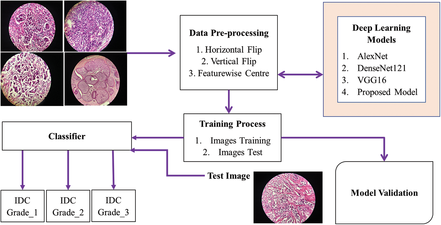
Figure 1: Proposed model flow chart

Fig. 2 illustrates the IDC DataBioX and BreaKHis dataset sample images. Fig. 3 shows the preprocessed images, including feature-wise center, horizontal flip, and vertical flip.

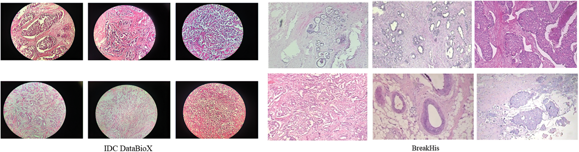
Figure 2: Sample images of IDC DataBioX and BreaKHis datasets

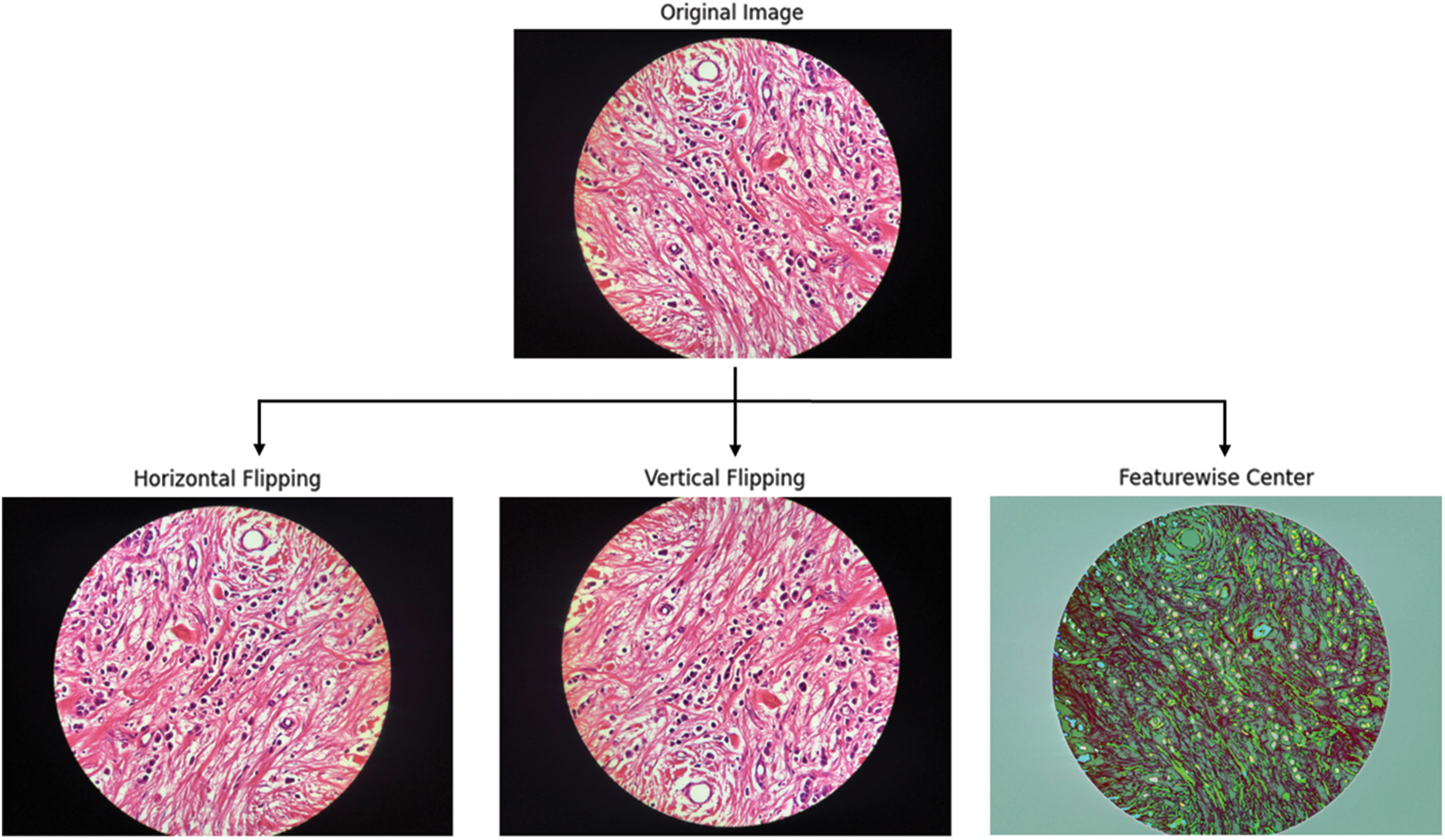
Figure 3: The steps of the horizontal flip, vertical flip, and feature-wise center

3.2 Training and Implementation

This study involved training a CNN model on the Google Colab platform over 50 epochs using one 12 GB NVIDIA Tesla K80 GPU with maximum continuous use. The GPU mode was utilized for faster execution, but the completion time of the training process depended on factors such as network speed and dataset size.

The proposed CNN model is optimized using the Adam optimizer with a default learning rate of 0.001, as it helps experiment and fine-tune the hyperparameters to find the most suitable optimizer for a task. Several vital parameters were used for effective training, including reduced learning rate, model checkpoint, and early stopping. The reduced learning rate helped adjust the learning rate dynamically based on the training progress. The validation accuracy was monitored, and it did not improve for five consecutive epochs with a minimum change of 0.0001; the current learning rate was reduced by half. This process continued until the last epoch. The model checkpoint callback was used to save the weights of the best-performing model based on validation accuracy. Early stopping was implemented to determine the total number of epochs for training. After 50 epochs, if no performance improvement was observed, the training process was stopped to avoid overfitting. For the hyperparameter, batch size was set to 4 in the ECAM, as it returned satisfactory results. Larger batch sizes allow for better parallelization but may lead to poorer generalization.

Softmax cross-entropy was utilized as the loss function, making it ideal for multiclass classification problems. This loss function measures any disparity between the network output and label output; to evaluate model performance, accuracy, precision, recall, and F1 score (β = 1) were used, these metrics being computed on true positives (TP), false positives (FP), true negatives (TN), and false negatives (FN) predicted by its predictions. Each case was subjected to the Softmax cross-entropy loss function at the Grade-1, Grade-2, and Grade-3 amplification levels, according to Eq. (1) [21,22], where yi denotes the target value. At the same time, f(x) represents the output from the activation function representing probability for each class. The performance metrics can be formulated for these four groups as shown in Eqs. (2)–(5).

CrossEntropy Loss =−∑i=1C⁡yilog⁡f(x)i(1)

Accuracy=TPcount + TNcount TPcount + TNcount + FPcount + FNcount(2)

Preision=TPcount TPcount+ FPcount(3)

Recall=TPcountTPcount+FNcount(4)

F1=TPcountTPcount+FPcount+FNcount(5)

Accuracy (Eq. (2)): This metric assesses the overall correctness of the model’s predictions. It is calculated by summing the counts of true positives (TP) and true negatives (TN) and dividing by the total number of predictions, including TP, TN, false positives (FP), and false negatives (FN). Precision (Eq. (3)): Precision measures the accuracy of positive predictions made by the model. It calculates the ratio of true positives (TP) to the sum of true positives (TP) and false positives (FP). Recall (Eq. (4)): Recall, also known as sensitivity or true positive rate, quantifies the model’s ability to identify positive cases correctly. It is calculated as the ratio of true positives (TP) to the sum of true positives (TP) and false negatives (FN). F1 score (Eq. (5)): The F1 score is the harmonic mean of precision and recall. It balances the trade-off between precision and recall and is particularly useful when dealing with imbalanced datasets. It is calculated as the ratio of true positives (TP) to the sum of true positives (TP), false positives (FP), and false negatives (FN).

3.3 Proposed Methodology

Our ECAM model introduces a new architecture with key components to enhance breast cancer diagnosis. The model's architecture consists of a separable CNN, channel-wise attention, and hierarchical feature aggregation, as shown in Fig. 4. This combination of design elements significantly improves the model’s performance. The model begins with an input layer image of 224 × 224 pixels with three color channels (RGB). The ECAM consists of four convolutional Groups (CG): CG-1, CG-2, CG-3, and CG-4. Each group comprises two convolutional blocks (CB) and one feature aggregation node. In CG-2 and CG-4 also apply a Squeeze and Excitation (SE) block in the ECAM. The model subsequently uses convolutional and pooling layers, with global average pooling for feature vector creation, followed by dropout for regularization and a dense layer for producing predictions in three-class classification tasks. The detail of the ECAM is described in Subsection 3.4.

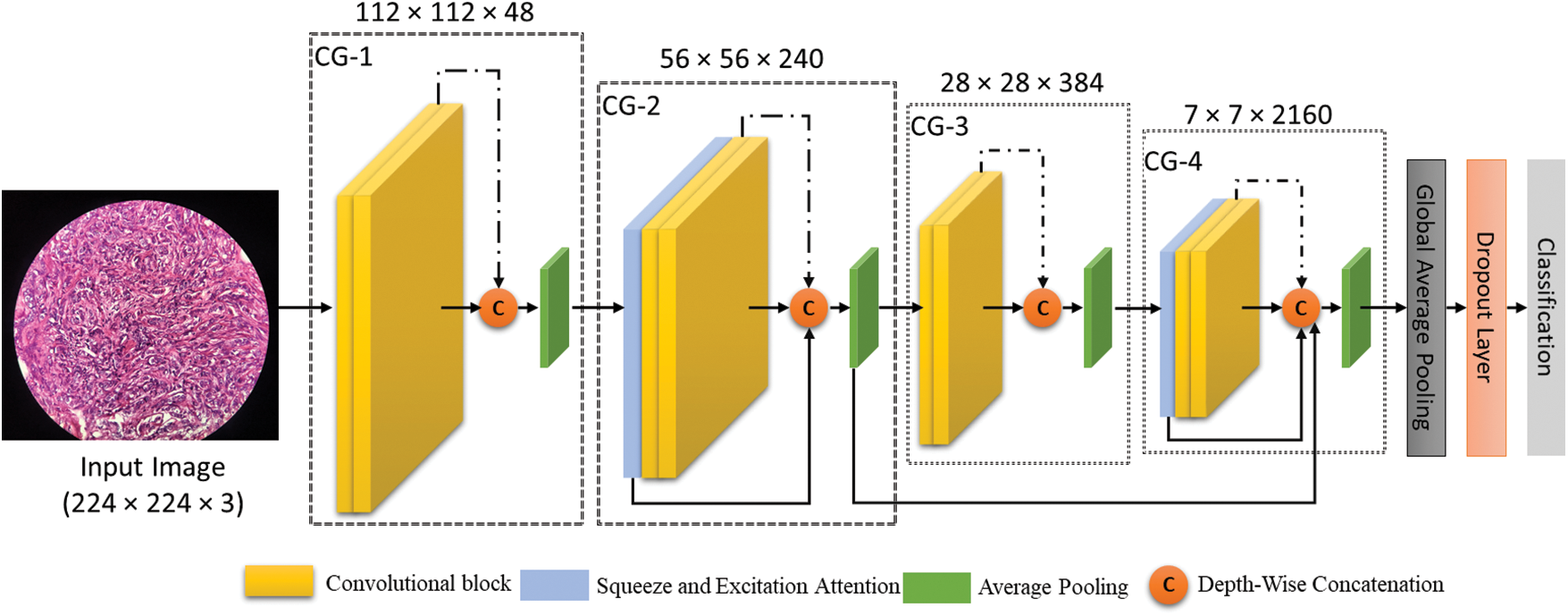
Figure 4: The proposed ECAM model (Convolution group-n is represented by CG-n in the ECAM)

3.4 Architecture of the ECAM Model

Researchers have developed models to improve DL network performance while minimizing learnable parameters associated with these networks. There is widespread agreement that including nonlinearity, better capacity, and broader receptive fields in a model would result in improved performance; however, this improvement will come at the expense of an increase in computational complexity [23]. Adding more depth or width to a network is not a surefire way to get the best benefits out of it. One of the biggest challenges DL engineers confront is managing shrink or explode gradients. Additionally, important are connections between the various levels and features. We investigated and tried many parts of DL to lower the number of factors that could be learned while improving accuracy. Below are the following details of these models.

3.4.1 Deep Aggregation of Features

CNNs contain many layers, each of which does something different. Compounding and merging layers are proactive measures to improve CNNs’ ability to enhance results; more than one division layer alone is insufficient. Researchers have made different CNN designs, from deeper to broader networks. It takes more than making it deeper or more comprehensive for the end layer to have the best qualities [23]. The proposed approach employs a sophisticated deep-learning-based architecture to address these issues, incorporating a hierarchical blending of data from various network levels.

The proposed model achieves its signature connected characteristics by combining light and deep layers in an aggregated fashion, with layers of comparable depths being aggregated together. They are added to the layer that is located above them. To avoid losing important data, the final feature map includes features from further network blocks using skip-connection techniques. Eq. (6) is a mathematical representation of how deep features are added together across layers in this method:

Fd=A((Rd−1d(x),Rd−2d(x),…,R1n(x),L1n(x),L2n(x))).(6)

Eq. (6) offers significant information about the ultimate feature map, named F. This feature map contains crucial details about the depth, feature map, and aggregation node of level x in the model. The variables L and R in Eq. (6), depict the hierarchical feature aggregation’s relationship between diverse feature maps. Eqs. (7) and (8) further illustrate this concept:

L2d(x)=C(L1d(x)),L1d(x)=C(R1d(x)),(7)

Rmd(x)={Fm(x),if m=n−1Fm(Rm+1d(x)),otherwise.(8)

Using residual connections is crucial for solving issues with gradients that either become too small or too large. Maintaining the hierarchy of these connections is important to avoid any negative impact on network performance [24]. Our proposed method involves performing feature aggregation at multiple levels. During training, this method helps minimize the chances of gradients diminishing or exploding, offering alternate short paths. This is represented by Eq. (9), which is shown here:

A(x1,…xd)=σ(BatchNorm(∑i⁡Wixi+b)),(9)

where σ shows nonlinear “activation that is not linear.” Wi and b in a CNN’s convolutional layer stand for biases and weights, respectively, and BatchNorm stands for batch normalization. Our suggested ECAM used eight convolution blocks. Models based on DL use convolutional layering as key building blocks to improve speed and reduce delay [24]. In Fig. 5, it is shown that each CB consists of two separate CL that use different kernel sizes (3 × 3–5 × 5). These levels help speed up performance and reduce delay simultaneously. Alex-Net and Dense-Net used convolution layers as usual.

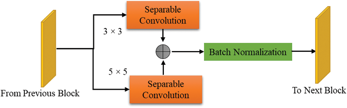
Figure 5: Single convolution block

Researchers have recently developed new ways to improve intelligence processing power, such as separate or group convolutions. One effective technique is to use depth-wise separate convolutions. This approach can significantly decrease the model’s size, time inference, and training parameters. Depthwise ECAM involves two stages: spatial convolution (for depthwise three-dimensional) and pointwise convolution. In Fig. 5, you can see a convolution block that uses kernels of sizes 3 × 3 and 5 × 5. This allows the use of multiscale data. The output of both separable convolution layers is merged through element-wise addition. Next, a batch normalization layer is applied to normalize them. We have implemented an aggregation last node to ensure seamless integration between the initial and final blocks. The performance of this node is genuinely remarkable, seamlessly combining the multiscale features from the separate layers. This innovative approach ensures a cohesive and synergistic fusion of these features, resulting in unparalleled performance. Channel-wise attention is implemented using SE blocks.

3.4.2 Use of the Squeeze Block and Excitation Block

To improve CNN, Hong et al. [23] proposed adding a new SE Block to CNNs to improve how they show features. A CNN offers the features of an image by using methods like convolutional neural layer pooling and batch normalization. Each part of its structure serves a specific purpose. A recent research focused on determining how feature maps connect to one another in space. Only a small amount of research has been done on channel-wise data. SE focuses on information about each channel, which helps improve performance without adding more factors that can be learned [24,25]. CNN use is standardized, and each station’s weight is given based on importance. Note that the SE is a flexible part that can be used or linked anywhere in a network. Starting with key elements that work for all classes, the following levels focus on more valuable elements that work for each class.

An SE block is comprised of three modules, which are labeled as follows: (a) the squeeze module, (b) the excitation module, and (c) the scale module, as shown in Figs. 6 and 7. The SE module combines feature maps based on 3 layers of dimensions to create a channel descriptor (H × W). Throughout the procedure, information is embedded in the system. Performing global average pooling squeezes the output to 1 × 1 × C, with C as the number of channels. The squeeze module output serves as input to the excitation part, which generates per-channel execution weights. The “excited” tensor has 1 × 1 × C dimensions and is output by the squeeze module. This matrix is then passed through a sigmoid activation layer to normalize the output between 0 and 1. The input is transformed using the sigmoid function before being element-wise multiplied with the output. Channel-wise weights are then applied to scale the output. In this way, new channels that have been recalibrated might be accessed. Fig. 6 shows all components of the new block SE, while Fig. 7 illustrates the various steps performed on the input tensor using the SE block.

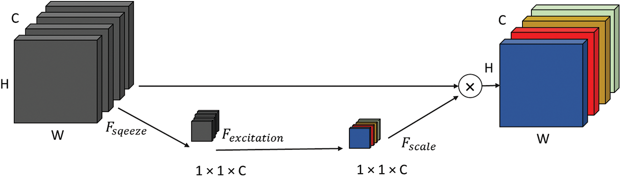
Figure 6: Proposed model includes a squeeze block and excitation block

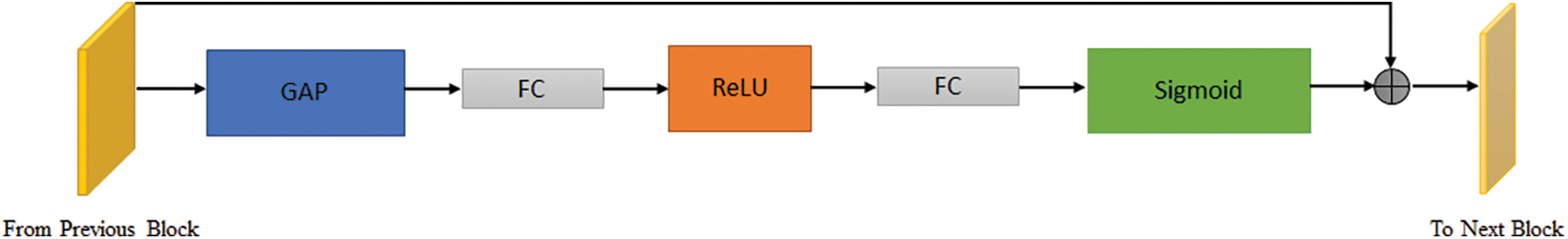
Figure 7: SE blocks carries out various operations

Eqs. (10)–(12) demonstrate the utilization of the squeeze, excitement, and scaling modules: If the output feature mappings U=([u1,u2,…,uC])ϵRH×W×C are created from the input tensor XϵRH′×W′×C′, after being transformed by Ftr, then

Fsqeeze(uc)=1H×W∑i=1H⁡∑j=1W⁡uc(i,j),(10)

where uc ϵRH×W is the result of the convolution process at the c-th element. The spatial dimension is shown by H and W. Eq. (11) shows how the excitement module can be described.

s=Fexcitation(z,W)=σ(g(z,W))=σ(W2Q(W1z)).(11)

In Eq. (11), the Q symbol represents the ReLU activation function. In this equation, W1ϵRCr×Cand W2ϵRCr×Cboth have the form RCr×C. Eq. (12) illustrates the ultimate outcome of the SE block following rescaling and activation:

X~=Fscale(uc,sc)=scuc,(12)

where X~=[X~1,X~2,…,X~C], and Fscale(uc,sc) this represents a scalar value. sc and for mapping the feature ucϵRH×W channel-wise multiplication.

The SE block is adaptable to any DL model. We incorporated it into our suggested method and achieved improved accuracy. The ECAM model’s layers are detailed in Table 1.

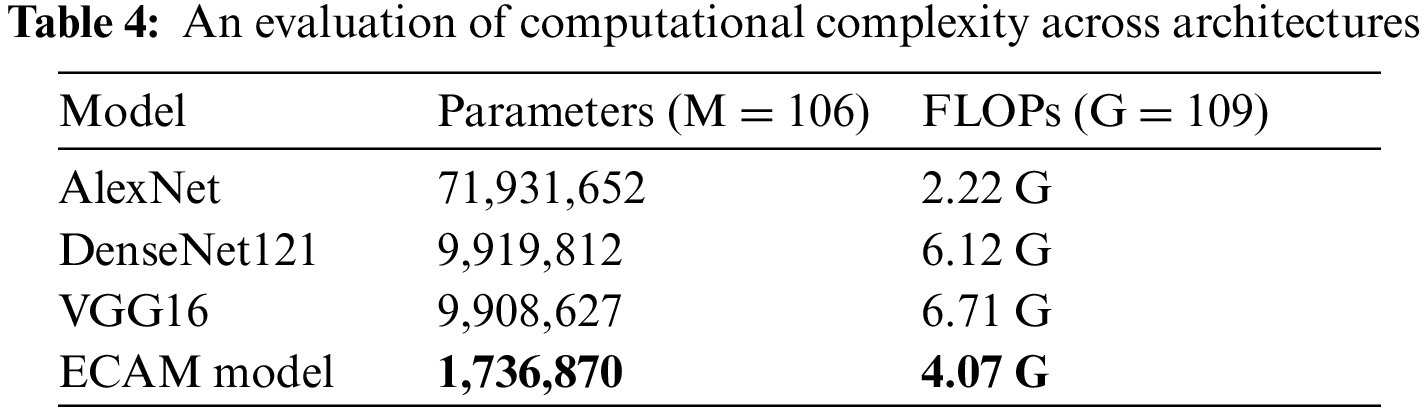
The ECAM model is a DL architecture designed for image classification with 1,736,870 parameters. It comprises separable convolutional layers to extract features, followed by batch normalization for regularization and scaling. The Model also includes concatenation layers to combine feature maps from different branches. Average pooling and global average pooling layers are used for downsampling and global feature extraction, respectively. Dense layers with activation functions are employed for the final classification. Dropout is utilized for regularization during training. The Model has four different output types and can do about 4.07 billion Floating Point Operations (Flops). Table 1 shows the specifics of the plan being proposed.

4  Results

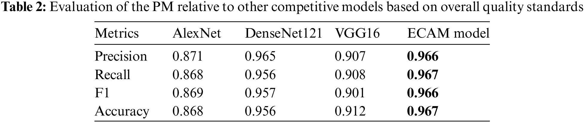
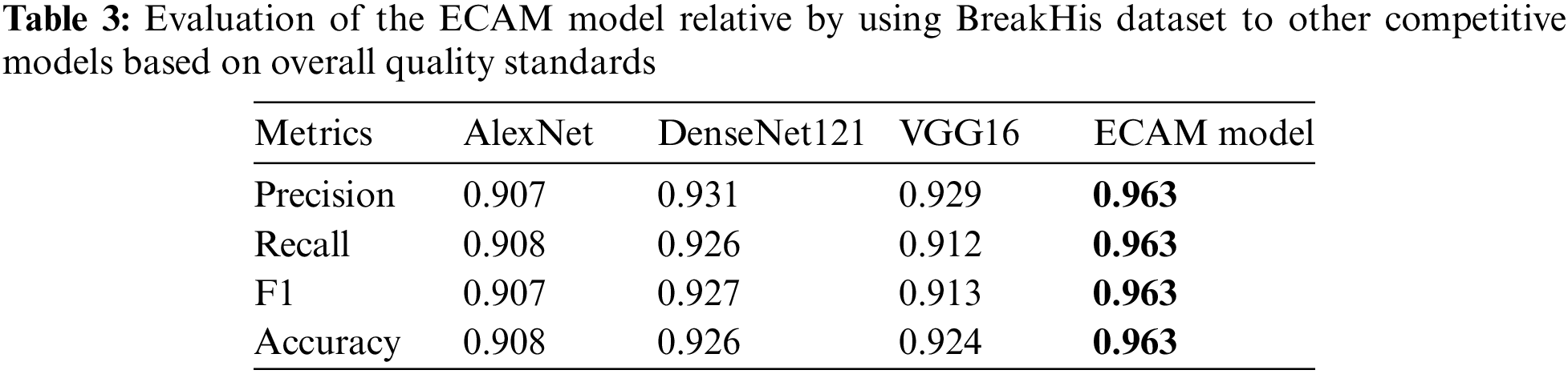
To evaluate the ECAM model objectively, its performance was assessed against that of DenseNet121, VGG16 and AlexNet. We used a range of quality metrics, including precision, recall, F1 score, and accuracy, to evaluate both the performance of the model and its individual class performance. Mainly, overall accuracy did not merely rely on class-wise accuracy but instead regarded as total instances of true positives (TP), true negatives (TN), false positives (FP), and false negatives (FN) across all classes, using Python’s sci-kit-learn library; consequently, the overall metric could even be lower than any individual class’s lowest metric obtained. Table 2 presents the performance comparison of various models used for classifying breast tissues from the IDC dataset. Table 3 presents the performance comparison of various models used for classifying breast tissues from the BreakHis dataset. Our ECAM model boasted an outstanding classification accuracy of 96.70%, and with BreakHis 96.33% surpassing all other models in this evaluation. Precision, recall and F1 score values for our ECAM model stood at 96.6%, and with BreakHis 96.37% respectively, while DenseNet121, VGG16 and AlexNet provided subpar performance compared with all the others tested.

Figs. 8 and 9 present the learning curves of our ECAM model applied on IDC DataBiox and BreakHis dataset, respectively. The graphs show that the training and validation curves are closely aligned, indicating that the training data accurately represents the validation data during testing. This alignment also suggests that the model is robust and could be applied to real-world scenarios with confidence. Fig. 10 shows the confusion matrix, and RoC curve of ECAM model on IDC DataBiox. Figs. 11 and 12 provides values insight into the learning performance of DenseNet121, VGG16 and AlexNet during training iterations cycles, offering practical perspectives into their performance during this training phase.

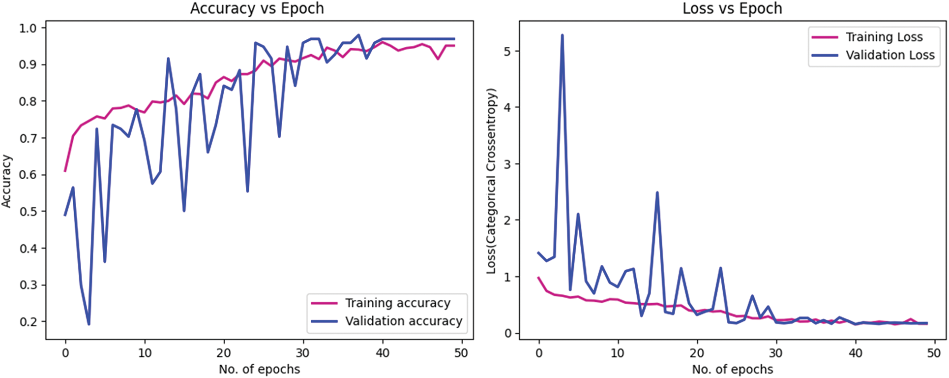
Figure 8: The ECAM model’s learning curve, including its training and validation accuracy, as well as the training and validation loss, are being examined by using IDC DataBiox dataset

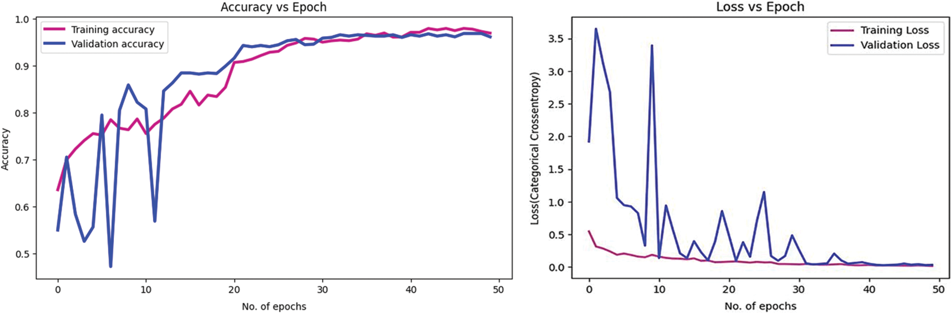
Figure 9: Learning curve of ECAM model with BreakHis dataset. Training and validation accuracy. Training and validation loss of an ECAM model

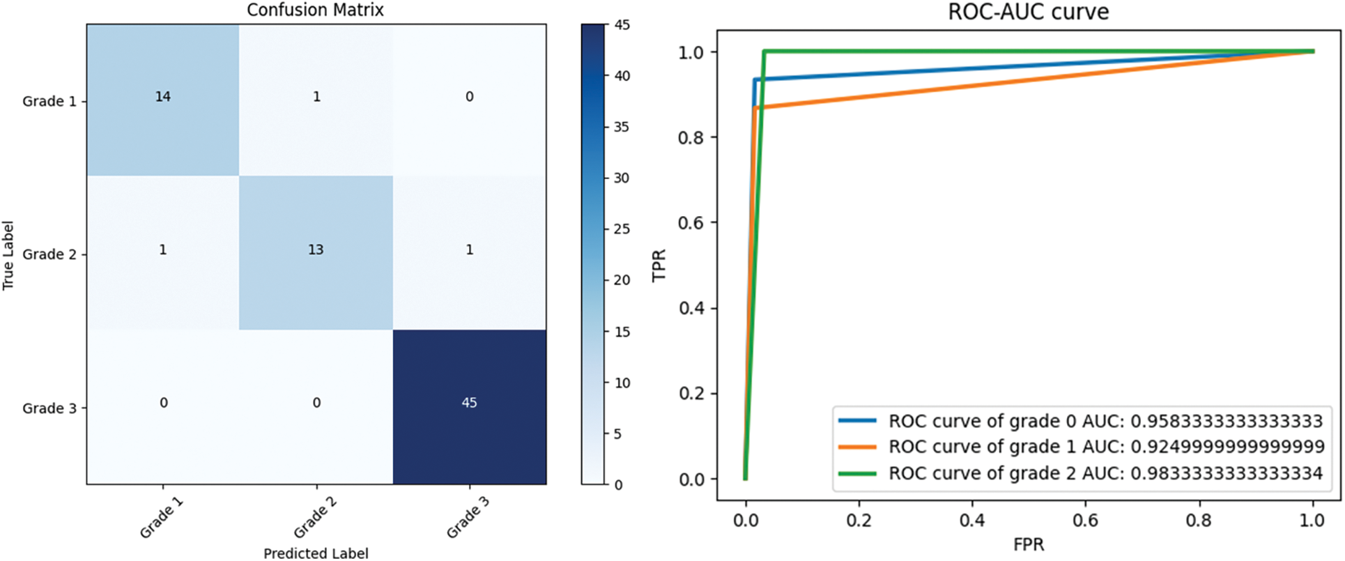
Figure 10: Confusion matrix, and RoC curve of ECAM model by using IDC DataBiox dataset

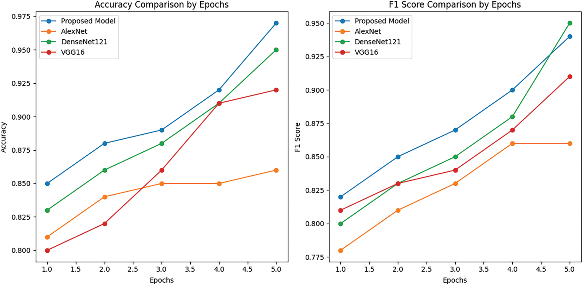
Figure 11: The ECAM model’s learning curve on the IDC DataBiox dataset is being examined, along with its training accuracy and F1 score compared to other models Densenet121, VGG16 and AlexNet

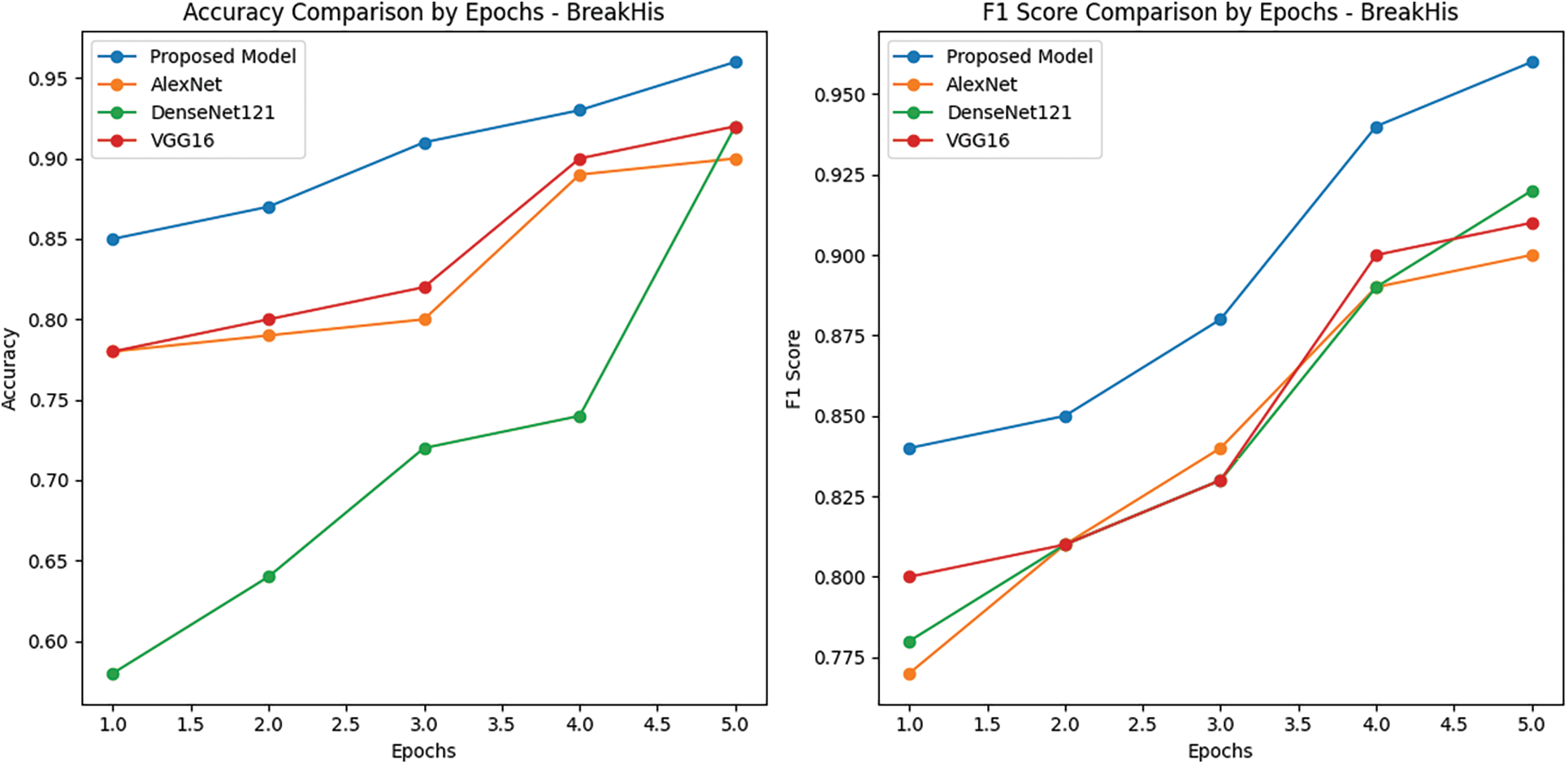
Figure 12: Learning curve of ECAM model on BreakHis dataset. Training accuracy and F1 score of ECAM model compared with other competitive Densenet121, VGG16 and AlexNet

Table 4 details the computational complexity of classification models using metrics such as trainable parameters and floating-point operations (FLOPs). The ECAM model and its reference models employ 0.3651 million parameters representing the lowest value out of all reference models; in comparison, AlexNet uses more parameters but requires the least number of FLOPs; DenseNetv121 and VGG16 requires the highest total FLOP count among these classification models.

5  Conclusions

This study introduces a novel DL model and conducts a comparative investigation into IDC classification using various pre-trained deep learning models, including DenseNet121, VGG16, AlexNet, and our ECAM model featuring deep feature aggregation and channel-wise attention. After being assessment using preferred quality metrics, our model achieved remarkable performance with an accuracy rate of 96.6% on the IDC dataset and 96.3% on the BreakHis dataset, as measured by the desired quality metrics. Especially, the F1 score soared to an impressive 96%, underscoring the model’s proficiency in accurately categorizing grades of breast cancer histopathology images. To measure its suitability for real-time applications, we conducted a thorough comparative analysis, scrutinizing factors such as inference time, model depth, memory utilization, and the number of parameters.

The paper utilized two medium-sized public datasets to conduct experiments. However, in order to verify the model’s generalization capabilities, cross-dataset experiments with a larger dataset are required. Moreover, it is crucial to conduct further testing with noisy data to evaluate the effectiveness of the model, considering potential variations in data during collection and preparation.

In our future work, our main focus will be on enhancing the accuracy of classification. Additionally, we intend to analyze the effect of other deep models on the performance of the ensemble model when dealing with large datasets. Moreover, we plan to consider all the historical data of the patient to provide more accurate inferences.

Acknowledgement: The authors would like to express their gratitude to Professor Dr. Wang Zhenfei and Professor Dr. Hou Weiyan for supervising of this study.

Funding Statement: The authors received no specific funding for this study.

Author Contributions: The authors confirm contribution to the paper as follows: study conception and design: Muhammad Mumtaz Ali, Faiqa Maqsood, Wang Zhenfei; data collection: Muhammad Mumtaz Ali, Liu Shiqi; analysis and interpretation of results: Muhammad Mumtaz Ali, Faiqa Maqsood, Hou Weiyan; draft manuscript preparation: Muhammad Mumtaz Ali, Faiqa Maqsood, Zhang Liying. All authors reviewed the results and approved the final version of the manuscript.

Availability of Data and Materials: The datasets can be accessed from IDC at: http://databiox.com and from BreakHis at: https://www.kaggle.com/datasets/ambarish/breakhis. The code and the outcomes of this study can be obtained from the corresponding authors upon a request. This option will be made available upon the publication of this work.

Conflicts of Interest: The authors declare that they have no conflicts of interest to report regarding the present study.

References

1. WHO, Breast Cancer. 2023. [Online]. Available: https://www.who.int/news-room/fact-sheets/detail/breast-cancer (accessed on 05/08/2023) [Google Scholar]

2. A. Cruz-Roa, A. Basavanhally, F. González, H. Gilmore, M. Feldman et al., “Automatic detection of invasive ductal carcinoma in whole slide images with convolutional neural networks,” in M. N. Gurcan, A. Madabhushi (Eds.SPIE Medical Imaging, pp. 904103, San Diego, California, USA: Spiedigitallibrary, 2014. [Google Scholar]

3. M. Veta, P. J. van Diest, R. Kornegoor, A. Huisman, M. A. Viergever et al., “Automatic nuclei segmentation in H&E stained breast cancer histopathology images,” PLoS One, vol. 8, no. 7, pp. e70221, 2013. [Google Scholar] [PubMed]

4. G. Yu, Z. Chen, J. Wu and Y. Tan, “A diagnostic prediction framework on auxiliary medical system for breast cancer in developing countries,” Knowledge-Based Systems, vol. 232, pp. 107459, 2021. [Google Scholar]

5. A. M. Khan, K. Sirinukunwattana and N. Rajpoot, “A global covariance descriptor for nuclear atypia scoring in breast histopathology images,” IEEE Journal of Biomedical and Health Informatics, vol. 19, no. 5, pp. 1637–1647, 2015. [Google Scholar] [PubMed]

6. A. Das, M. S. Nair and S. D. Peter, “Sparse representation over learned dictionaries on the riemannian manifold for automated grading of nuclear pleomorphism in breast cancer,” IEEE Transactions on Image Processing, vol. 28, no. 3, pp. 1248–1260, 2019. [Google Scholar] [PubMed]

7. S. Naik, S. Doyle, S. Agner, A. Madabhushi, M. Feldman et al., “Automated gland and nuclei segmentation for grading of prostate and breast cancer histopathology,” in 5th IEEE Int. Symp. on Biomedical Imaging: Nano to Macro, Paris, France, pp. 284–287, 2018. [Google Scholar]

8. T. Wan, J. Cao, J. Chen and Z. Qin, “Automated grading of breast cancer histopathology using cascaded ensemble with combination of multi-level image features,” Neurocomputing, vol. 229, pp. 34–44, 2017. [Google Scholar]

9. G. Maguolo, L. Nanni and S. Ghidoni, “Ensemble of convolutional neural networks trained with different activation functions,” Expert Systems with Applications, vol. 166, pp. 114048, 2021. [Google Scholar]

10. H. Bolhasani, E. Amjadi, M. Tabatabaeian and S. J. Jassbi, “A histopathological image dataset for grading breast invasive ductal carcinomas,” Informatics in Medicine Unlocked, vol. 19, pp. 100341, 2020. [Google Scholar]

11. Y. Benhammou, B. Achchab, F. Herrera and S. Tabik, “BreakHis based breast cancer automatic diagnosis using deep learning: Taxonomy, survey and insights,” Neurocomputing, vol. 375, pp. 9–24, 2020. [Google Scholar]

12. N. Brancati, G. de Pietro, M. Frucci and D. Riccio, “A deep learning approach for breast invasive ductal carcinoma detection and lymphoma multi-classification in histological images,” IEEE Access, vol. 7, pp. 44709–44720, 2019. [Google Scholar]

13. N. A. Barsha, A. Rahman and M. R. C. Mahdy, “Automated detection and grading of Invasive Ductal Carcinoma breast cancer using ensemble of deep learning models,” Computers in Biology and Medicine, vol. 139, pp. 104931, 2021. [Google Scholar] [PubMed]

14. A. M. Romano and A. A. Hernandez, “Enhanced deep learning approach for predicting invasive ductal carcinoma from histopathology images,” in 2nd Int. Conf. on Artificial Intelligence and Big Data (ICAIBD), Chengdu, China, IEEE, pp. 142–148, 2019. [Google Scholar]

15. A. Janowczyk and A. Madabhushi, “Deep learning for digital pathology image analysis: A comprehensive tutorial with selected use cases,” Journal of Pathology Informatics, vol. 7, no. 1, pp. 29, 2016. [Google Scholar] [PubMed]

16. R. Sujatha, J. M. Chatterjee, A. Angelopoulou, E. Kapetanios, P. N. Srinivasu et al., “A transfer learning-based system for grading breast invasive ductal carcinoma,” IET Image Processing, vol. 17, no. 7, pp. 1979–1990, 2023. [Google Scholar]

17. Y. Celik, M. Talo, O. Yildirim, M. Karabatak and U. R. Acharya, “Automated invasive ductal carcinoma detection based using deep transfer learning with whole-slide images,” Pattern Recognition Letters, vol. 133, pp. 232–239, 2020. [Google Scholar]

18. Y. Hao, L. Zhang, S. Qiao, Y. Bai, R. Cheng et al., “Breast cancer histopathological images classification based on deep semantic features and gray level co-occurrence matrix,” PLoS One, vol. 17, no. 5, pp. e0267955, 2022. [Google Scholar] [PubMed]

19. M. A. Islam, D. Tripura, M. Dutta, M. N. R. Shuvo, A. F. Wasik et al., “Forecast breast cancer cells from microscopic biopsy images using big transfer (BiTA deep learning approach,” International Journal of Advanced Computer Science and Applications, vol. 12, no. 10, 2021. [Google Scholar]

20. F. Parvin and Md. A. Mehedi Hasan, “A comparative study of different types of convolutional neural networks for breast cancer histopathological image classification,” in IEEE Region 10 Symp. (TENSYMP), pp. 945–948, 2020. [Google Scholar]

21. V. Badrinarayanan, A. Kendall and R. Cipolla, “SegNet: A deep convolutional encoder-decoder architecture for image segmentation,” IEEE Transactions on Pattern Analysis and Machine Intelligence, vol. 39, no. 12, pp. 2481–2495, 2017. [Google Scholar] [PubMed]

22. S. Lal, D. Das, K. Alabhya, A. Kanfade, A. Kumar et al., “NucleiSegNet: Robust deep learning architecture for the nuclei segmentation of liver cancer histopathology images,” Computerized Medical Imaging and Graphics, vol. 128, pp. 104075, 2021. [Google Scholar]

23. S. B. Hong, Y. H. Kim, S. H. Nam and K. R. Park, “S3D: Squeeze and excitation 3D convolutional neural networks for a fall detection system,” Mathematics, vol. 10, no. 3, pp. 328, 2022. [Google Scholar]

24. Md. M. K. Sarker, F. Akram, M. Alsharid, V. K. Singh, R. Yasrab et al., “Efficient breast cancer classification network with dual squeeze and excitation in histopathological images,” Diagnostics, vol. 13, no. 1, pp. 103, 2022. [Google Scholar] [PubMed]

25. M. Ayoub, Z. Liao, S. Hussain, L. Li, C. W. J. Zhang et al., “End to end vision transformer architecture for brain stroke assessment based on multi-slice classification and localization using computed tomography,” Computerized Medical Imaging and Graphics, vol. 109, pp. 102294, 2023. [Google Scholar] [PubMed]