An Intelligent Approach for Intrusion Detection in Industrial Control System

1  Introduction

The Industrial Control System is a control system for industrial production, and is an important part of national infrastructure, widely used in key fields such as water conservancy, nuclear power, and energy, as the core control equipment of national infrastructure; its security is related to the national economy and people’s livelihood [1].

With the fast growth of industrial control systems, which are now extensively employed, security problems are becoming more common. The “Stuxnet” virus outbreak in 2010 immediately caused substantial damage to the centrifuges of Iran’s nuclear plants. After the Stuxnet virus spread, the industrial control system eventually became one of the primary targets of attackers [2]. The global WannaCry ransomware epidemic in 2017 made use of the high-risk vulnerability “Eternal Bule” to spread globally, disrupting major businesses such as energy, transportation, and communications in many nations [3]. In March 2018, the United States Computer Emergency Preparedness Team issued security warning TA18-074A, which detailed a cyber-attack on a power facility in the United States by Russian hackers. The goal of this attack is to gather intelligence and record pertinent information for the computer implantation programmed to attack, resulting in massive losses for the power plant [4]. In 2019, a network targeted the computer system control center of the Guri Hydropower Station, Venezuela’s largest power plant, creating a statewide power outage and affecting around 30 million people. The Guri Hydropower Station in Venezuela was attacked again in July of the same year, resulting in widespread outages in 16 states, including Lagas [5]. Because industrial control systems are such an important aspect of national infrastructure, assaults on them frequently result in more significant consequences and bigger economic losses.

Given the security dangers to the industrial control system, using intrusion detection measures to defend is a critical step. Now, various elements of intrusion detection based on the industrial control system are being explored, and intelligent detection of infiltration of the industrial control system is accomplished by combining the machine-learning model. Among the different machine learning models, the one-class support vector machine (OCSVM) model requires just one sort of data on the training data, allowing it to detect unknown intrusions, and as a result, it has become a popular approach for intrusion detection in industrial control systems. Due to the lack of negative example training data, the trained model will have a high FPR (False Positive Rate), therefore this work provides the learning model for intrusion detection, trains the model using regular traffic as positive example label data, and retains the model for unknown intrusions. While enhancing the model’s detection ability, the model’s intrusion detection ability is enhanced. Because the suggested learning model employs both a class of labeled data and unlabeled data to be identified for model training, its classification performance is frequently superior to that of the anomaly detection model.

The main contributions of this paper can be summarized as follows:

•   Because the trained model will have a high FPR (False Positive Rate) due to a lack of negative example training data, this work supplies the learning model for intrusion detection, trains the model using ordinary traffic as positive example label data, and retains the model for unknown intrusions. The model’s intrusion detection ability is improved while its detection ability is improved. Because the proposed learning model uses both labeled and unlabeled data to train the model, its classification performance is typically superior to that of the anomaly detection model.

•   This paper analyses the class prior probability estimation algorithm based on the positive label frequency, divides the reliable positive example set through the one-class SVM model, improves the calculation method of the positive label frequency, and reduces the error in the prior probability estimate is small.

•   Based on the concealment characteristics of industrial control system attacks, positive unlabeled learning is applied to the intrusion detection of industrial control systems, a neural network is built for learning, and the classification model is trained using only normal traffic as label data, and a public data set experiment is performed. Experiments confirm the model’s efficacy.

This paper is structured as follows. Section 2 presents the research status of intrusion detection and positive unlabeled learning in industrial control systems. Section 3 is the main research content of this paper. Section 4 verifies the effectiveness of the proposed algorithm through experiments. Section 5 summarizes the article.

1.1 Symbols and Notation

Table 1 lists the symbols and corresponding descriptions.

2  Related Work

2.1 Overview of Industrial Control System

From top to bottom, the industrial control network layer model is separated into five layers: enterprise resource layer, production management layer, process monitoring layer, field control layer, and field device layer. The requirements for real-time depend on the layer. As indicated in Fig. 1, the enterprise resource layer primarily consists of the functional units of the ERP system that are utilized to offer decision-making operation methods for the employees of the enterprise decision-making layer.

Figure 1: Industrial control system architecture

The field device layer is the lowest level of industrial control and contains certain field devices such as sensors, monitors, and other execution equipment units that are used to perceive and run the production process.

Field devices are monitored and controlled using the process monitoring layer and the field control layer. SCADA and HMI are the primary components of the process monitoring layer. SCADA may monitor and operate on-site operational equipment to perform data acquisition, equipment control, measurement, parameter modification, and other operations. HMI stands for human-machine interface, and it is used to communicate information between the system and the user. The on-site control layer is mostly PLC, which communicates with the HMI, receives control orders and query requests and communicates with field devices, controlling them by delivering operation instructions.

The production management layer includes MES and MOMS, which are used to manage the production process, such as manufacturing data management, production scheduling management, etc.

The top layer is the enterprise resource layer, where the enterprise resource planning (ERP) system manages core business processes, such as production or product planning, material management, and financial conditions.

2.2 Features of Intrusion Detection in Industrial Control System

There are significant differences between the intrusion detection of industrial control systems and the intrusion detection of the Internet. Due to the particularity of the environment of industrial control systems, it has unique characteristics [6]:

•   High real-time performance. Industrial control systems are usually deployed in fields such as electric power and nuclear energy, and the systems have high real-time performance, so intrusion detection also requires high real-time performance.

•   The resources of industrial control equipment are limited. Industrial control systems contain a large number of sensors and actuators that perform specific operations. To reduce costs, their computing and storage resources are usually very limited.

•   The device is difficult to update and reboot. The industrial control system is closely connected with the physical world, and it is usually impossible to suspend work, otherwise, it will cause serious harm to the entire industrial control system, personnel, and the environment.

Based on the characteristics of the above industrial control system, higher requirements are put forward for the intrusion detection system:

•   Real-time. Industrial control systems have higher real-time requirements for intrusion detection, requiring intrusion detection systems to use real-time information from industrial control systems for intrusion detection.

•   Resources are limited. The limited resources of the industrial control system restrict the methods of intrusion detection and require the intrusion detection model to have low resource consumption. The time complexity of some algorithms based on deep learning is relatively high, especially the deep learning model, regardless of the training time, some deep neural network models have a very large number of complex network structure parameters, and the required training and prediction time is also longer. In the case of resources first, some complex deep neural network models are difficult to apply to intrusion detection of industrial control systems. Therefore, when applying the neural network model to the intrusion detection of industrial control systems, it is necessary to focus on the complexity of the model and make the neural network structure as simple as possible while ensuring accuracy.

•   The device is difficult to update and restart. This feature limits the performance of intrusion detection models. First of all, because it is difficult for the equipment to update the model, it needs to have good generalization performance, that is, the model trained on the training data also needs to have good performance when applied to the real data. The second is the requirement of indicators. Since the device cannot be restarted or suspended, it is necessary to have a high precision rate for intrusion detection, that is, it is better to miss than to falsely report.

The above are the characteristics of industrial control systems. When performing intrusion detection, it is usually necessary to analyze based on its traffic. The characteristics of industrial data are high dimensionality and strong correlation, which will increase the training time of the intrusion detection model. Therefore, it is necessary to analyze the industrial data Feature extraction reduces the complexity of subsequent data modeling and processing.

Based on the requirements of high precision rate and low resource consumption of industrial control systems, as well as the difficulty of obtaining data labels, this paper constructs a shallow neural network for PU learning, which is used for intrusion detection of industrial control systems. At the same time, given the high dimensionality and strong correlation of industrial control system data, a feature selection algorithm based on PU learning is proposed for data dimensionality reduction.

2.3 Literature of Intrusion Detection Methods in Industrial Control Systems

Industrial control system intrusion detection can be divided into traffic-based detection, device state-based detection, and protocol-based detection. In terms of traffic, construct features through the real traffic of the industrial control system, such as flow duration, port, and other information, and then combine some machine learning models for detection, such as one-class support vector machine (SVM) [7]. In terms of equipment status, reference [8] proposed an intrusion detection method based on the CUSUM algorithm. In this method, the difference between the actual value obtained by the sensor and the predicted value of the model is used as the statistical sequence, and the offset is designed according to the 3σ principle. The constant determines the threshold, and finally, the method is verified in experiments to effectively detect deviation attacks and geometric attacks. In terms of protocols, some industrial control protocols are open, and detection rules can be formulated according to the specifications of these protocols to detect specific industrial control protocols, such as the Modbus protocol [8,9].

With the rapid development of machine learning and artificial intelligence, its influence gradually radiates to the field of intrusion detection. A large number of machine learning models are used for intrusion detection. Different applicable machine learning algorithms can be divided into traditional classification models and clustering models [10,11], ensemble models, anomaly detection models, and neural networks. Due to the rapid development of neural networks and better classification performance than traditional machine learning models, intrusion detection based on traditional classification models is gradually cooling down. The integrated model and the anomaly detection model have their characteristics. The integrated model has better classification performance by integrating multiple base classifiers, and it is like a random forest [12]. The advantages of anomaly detection such as OCSVM are: 1) It can detect unknown intrusions; 2) Only background traffic is required as training data. With the deepening of research, neural networks such as autoencoders are used for unsupervised anomaly detection [13].

The most commonly used anomaly detection algorithm for intrusion detection is OCSVM. Reference [14] investigated the application of a one-class SVM algorithm in the intrusion detection of industrial control systems. On the network layer and the transport layer, the OCSVM algorithm is used for TCP/IP traffic anomaly detection of the SCADA system. On the application layer, the OCSVM model is trained based on the normal communication flow of ModbusTCP for intrusion detection. At the same time, the paper also pointed out that there are three main problems in OCSVM anomaly detection: Industrial control system problem of feature construction, parameter optimization, and high false positive rate.

Dynamic control center architectures are vulnerable to a variety of potentially active and passive cyber-attacks, as already explored by various industrial control protocols such as IEEE C37.118, IEC 61850, DNP3, IEC-104c, which put a variety of power system assets, such as RTUs, PMUs, protection systems, or relays, as well as control room servers, in danger. MITM attacks, data spoofings (such as inserting fake commands to trip lines or manipulating PMU measurement information), eavesdropping, or reconnaissance assaults are examples of common active or passive attack types. Intrusion detection systems (IDSs) enable the detection of unlawful activities or occurrences in ICT systems and reduce cyberattacks on vital infrastructures as a common defensive strategy. To identify cyber-attacks occurring during the PMU data transmission based on the IEEE C37.118 protocol, specification-based NIDS with a variety of stateful or stateless deep packet inspections are provided.

Compared with classic anomaly detection models such as one-class SVM, the deep learning model has improved the detection rate, but it takes longer to train the model.

Table 2 summarizes the work related to intrusion detection of industrial control systems based on machine learning in recent years. From the analysis of related work, the research on intrusion detection of industrial control systems has the following trends:

•   Tend to anomaly detection. The intrusion detection of industrial control systems is more often treated as an anomaly detection problem. In terms of model selection, a classification model such as one-class SVM or an unsupervised model such as AE is preferred for identification [15].

•   Tend to high precision. In recent years of research work, some researchers tend to optimize model parameters through some parameter optimization algorithms such as Particle Swarm Optimization (PSO) and Gravitational Search Algorithm (GSA), so that the model has better classification performance.

•   Tend to be real-time and efficient. Due to limited resources, the industrial control system requires the model to have a small calculation cost. From the perspective of related work, the intrusion detection of industrial control systems pays more attention to the model with low calculation consumption. At the same time, most of the models are trained through feature selection or feature extraction methods, such as principle component analysis (PCA) and fisher score for dimensionality reduction, thereby reducing the time and computation required for model training. The long-short memory network (LSTM) is also compared.

2.4 Positive Unlabeled Learning

Positive unlabeled learning is a neural network-based anomaly detection approach that estimates the binary classification error using positive and unlabeled data sets, allowing the positive unlabeled learning model to attain classification performance similar to the binary classification model. Because positive unlabeled learning requires training the model with both positive and unlabeled data sets, the unlabeled data set must first estimate the mixing ratio of positive and negative samples before applying it to positive unlabeled learning [31,32], also known as class prior estimation. The main method of class prior probability estimation is to start from the distribution of the positive unlabeled data set. The distribution of the unlabeled data set is a combination of the positive data distribution and the negative data distribution, the class prior probability can be obtained by comparing the distribution of positive unlabeled data sets [33–35]. In addition, the class prior probability estimation algorithm based on the positive label frequency is one of the most advanced algorithms at present. Reference [36] proposed the TICE algorithm, which divides reliable positive examples in the unlabeled data set Estimate the frequency of positive labels, which is currently the algorithm with the lowest time complexity.

Reference [37] first theoretically analyzed the positive unlabeled learning problem, compared positive unlabeled learning with the binary classification model, and estimated the loss of the binary classification sample under the condition of known class prior probability π, theoretically can obtain the same decision surface as the binary classification model, which is called uPU (unbiased Positve-unlabeled learning). Because the loss function of the uPU model needs to satisfy the symmetric condition, reference [38] continued to carry out research, gave a method of applying the loss function that does not satisfy the symmetric condition to the uPU, and verified the non-convex loss function and the convex loss function functions have similar precision.

Reference [39] further compared the positive unlabeled learning model with the binary classification model and analyzed the reasons why the positive unlabeled learning model performed better than the binary classification model in some cases.

Reference [40] proposed the nnPU (Positive-unlabeled learning with Non-negative risk estimator) algorithm to solve the problem that uPU is prone to overfitting. Based on uPU, it estimated the binary classification loss method to change. Furthermore, it ensures that the estimated negative example loss is always positive, thereby avoiding the problem caused by the estimated loss being negative, and points out that the performance of nnPU is better than that of uPU. Finally, reference [41] summarized the existing positive unlabeled learning and analyzed the seven main problems of positive unlabeled learning in the article, including the assumptions of positive unlabeled learning, evaluation indicators, main models, and class priors.

3  Proposed Intrusion Detection Learning Mechanism

The problem of intrusion detection in industrial control systems has received the attention of scholars as an anomaly detection problem, but some classic anomaly detection algorithms such as the one-class SVM algorithm have a high false positive rate, and the classification performance has a large gap compared with the binary classification model. This paper proposes to use positive unlabeled learning for intrusion detection. This method has been proved to have classification performance close to binary classification, and at the same time, it only needs one type of label data on the training data like the one-class SVM model.

The intrusion detection process based on positive unlabeled learning is shown in Fig. 2. In feature engineering, it is necessary to analyze features through positive label data and wrong label data, select key features, reduce data dimensions, and reduce the impact of irrelevant features on model classification performance. At the same time, the class prior probability of positive unlabeled learning is used as prior knowledge, which needs to be processed at the same time as feature engineering. By analyzing positive data and mislabeled data, a model is built to estimate the class prior probability of mislabeled data sets. Then combine the positive label data, unlabeled data, and class prior probability after feature selection to train the positive unlabeled learning model, and finally output the classification label of the model and the mislabeled data set.

Figure 2: Proposed algorithm flowchart

Based on the above process, the main research content of this part is divided into three parts: First, explore a feature selection algorithm based on positive unlabeled learning, and analyze the importance of features based on positive label data and unlabeled data. Secondly, research class prior probability estimation algorithm, improve the accuracy of class prior probability estimation and provide important prior knowledge for positive unlabeled learning. Finally, based on the data after feature selection and the estimated class prior probability, the classification model is trained by positive unlabeled learning.

In this paper, the problems of anomaly detection are answered in a targeted manner:

•   In terms of feature engineering, this paper studies the calculation method of feature importance based on positive unlabeled learning, which can be used as a feature selection metric for feature selection of industrial control system data;

•   In terms of resource constraints and real-time issues in industrial control systems, this paper chooses a shallow neural network, which requires less storage resources and computing resources, which meets the needs of industrial control systems;

•   In terms of false alarm rate, positive unlabeled learning has been shown to perform similarly to the binary classification model and to have a higher accuracy rate than the unsupervised anomaly detection model.

3.1 Feature Importance

In industrial control systems, data has the characteristics of high dimensionality and strong correlation. Many machine learning problems become difficult when the data dimensionality is high, a phenomenon known as the curse of dimensionality. Feature selection is an important part of feature engineering. Its principle is to extract key features from all features, to achieve the purpose of dimensionality reduction. Feature selection methods can be divided into two categories: encapsulation and filtering. Among them, the encapsulation feature selection usually selects a base model for multiple rounds of training and gradually screens out redundant features according to the classification performance of the trained model. Filtering feature selection is to calculate the importance of features, set a threshold to filter out irrelevant features, and further filter out redundant features through correlation.

In positive unlabeled learning, since there is only one class of labeled samples, it is difficult to evaluate the performance of the packaged model. Therefore, the filtering feature selection method is used in this paper. The commonly used feature importance calculation methods are shown in Table 3.

The importance calculation method of the filtering feature selection method is calculated by evaluating the correlation between features and labels, and it is considered that the features that have an obvious correlation with the target category are the key features. However, in positive unlabeled learning, there is only one class of labeled samples, and the feature importance calculation method in the binary classification model cannot be directly used. Therefore, it is necessary to find a feature importance calculation method suitable for positive unlabeled learning scenarios.

Inspired by the importance calculation idea of this binary classification, this paper presents a key feature identification method for PU learning: Considering that the unlabeled data set is a mixture of positive samples and negative samples, the attribute value of the feature in the unlabeled data set includes two parts: the positive value and the negative value. If the feature is strongly related to the class label, then the unlabeled data distribution of attribute values of this feature should show obvious bimodal or multimodal features and the distribution of different class sample features is quite different, as shown in Fig. 3. When the feature is weakly correlated with the class label, the positive sample similar to the feature distribution of the negative samples.

Figure 3: Comparison of feature relation of data correlation

The distribution difference of the feature on the positive data set and the unlabeled data set can be used as the importance of the feature. The Kullback–Leibler (KL) divergence can describe the difference between two distributions, and its discrete form is shown in formula (1).

KL(P||U)=∑P(x)log⁡(P(x)U(x))(1)

The KL divergence requires the probability of a feature attribute value when calculating the difference between two feature distributions. First of all, considering that the value range of the attribute value of the feature is not limited, it is necessary to standardize the maximum and minimum values before the calculation, to limit the attribute value after normalization to the [0,1] interval. Secondly, there are two forms of continuous and discrete attribute values of features. To deal with them uniformly, the [0,1] interval is equally divided in the algorithm, and the KL divergence is calculated by using the frequency of samples in each small area as a probability. The specific steps are shown in Algorithm 1.

Time complexity analysis: In the third step of the algorithm, data standardization is carried out, and the data standardization method adopted is the standardization of maximum and minimum values, and the time complexity of this step is O(mn). Steps 4 to 6 are to calculate the feature’s importance. By dividing the [0,1] interval into equal parts, the KL divergence is calculated with the frequency in each small interval as the probability. The time complexity of this part is O(mn). So the total time complexity of the algorithm is O(mn).

Through KL divergence, the estimated value of feature importance can be given in the scene with only positive label data, and key features can be distinguished from irrelevant features. In the case of redundant features, features can be filtered based on feature importance, such as setting feature importance thresholds or specifying the number of selected features.

3.2 Class Prior Probability Estimation for PU Learning

In the industrial control system, it is very difficult to collect a large amount of intrusion data, but the collection of traffic and status codes in the normal operation of the system is relatively simple. Taking the data in the normal state as the positive label data for positive unlabeled learning is in line with the actual situation of the industrial control system. In positive unlabeled learning, it is very important to analyze the data to be detected and obtain the class prior probability. The class prior probability of positive unlabeled learning is defined as π=p(y=1), when the collection of samples satisfies the SCAR (select at completely random) assumption, the class prior probability is the proportion of positive samples in the unlabeled data set proportion.

Definition 1 (SCAR assumption): The collection of samples has nothing to do with the attributes of the samples and is completely random, namely:

p(s=1|y)=p(s=1|x,y)(2)

According to the different sources of positive data, it can be divided into two categories: One Sample (OS) and Two Samples (TS). When the OS collects data, it only performs random sampling once, that is, randomly collects a part of the data in the real data, digs out some positive data from the collected data and adds labels, and unlabeled data as unlabeled data. When TS collects data, it needs to sample twice, that is, first randomly collect a part of the positive label data, and the unlabeled data set is obtained by random sampling in the real data.

Since the positive data is randomly selected in the unlabeled data set, an intermediate variable c is generated in this scenario, which is called the positive label frequency (label frequency), which is defined as c=p(s=1|y=1), where s=1 represents the sample that the sample is selected from. The relationship between label frequency and class prior probability can be expressed by Eq. (3).

p(y=1|x)=1cp(s=1|x)(3)

Therefore, the class prior probability can be estimated by estimating the positive label frequency c. In particular, in the TS scenario, the positive data and unlabeled data can be mixed, the positive samples can be regarded as randomly selected and labeled positive samples, and the frequency of positive labels can also be estimated.

The lower bound of the estimated positive label frequency is obtained by using the decision tree to obtain the estimated value of the positive label frequency. This algorithm is called the TIcE algorithm. In this paper, the one-class SVM algorithm is used to improve the TIcE algorithm, and the one-class SVM algorithm is proposed to divide the reliable positive example set, and then estimate the positive label frequency.

The one-class SVM algorithm is a classic anomaly detection algorithm. When it uses the RBF kernel function, its performance is similar to that of support vector data description (SVDD). It can be considered that the one-class SVM algorithm finds a hypersphere in the feature space, contains the positive samples in the hypersphere, and makes the radius of the hypersphere the smallest. Its problem description is shown in formula (4).

{min:12wTw−ρ+1vN∑i=1Nξis.t.wx≥ρ−ξi,ξi≥0,|w|=1(4)

The v in the formula is the upper bound of the proportion of outliers, so the number of samples classified as outliers in the positive data set can be limited by setting parameters so that the estimated deviation is caused by the small number of positive samples in the model division. At the same time, when the upper bound of the proportion of abnormal points is set larger, the radius of the hypersphere at this time is smaller, and the samples classified as positive by the model can be used as reliable positive samples.

On the estimation of positive label frequency, the estimated value can be given by Chebyshev’s inequality. Through Chebyshev’s inequality, the number LS of labeled samples in the positive example set S satisfies the formula (5).

P(|LS−μ|≥ε)≤σ2ε2(5)

where LS obeys the binomial distribution, and the expectation of the random variable LS is E(L)=cNS, the variance is D(L)=c(1−c)NS, and NS is the total number of samples in the positive example set S. Substitute into formula (5) to get:

P(|LS−cNS|≥ε)≤c(1−c)NSε2(6)

Let δ=c(1−c)NS/ε2, then formula (6) is equivalent to:

P(|LS−cNS|≤c(1−c)NSδ)≤δ(7)

Through the formula (7), the upper and lower bounds of the positive label frequency c can be constrained by the probability δ, as shown in the formula (8).

{P(c≤LSNs+c(1−c)δNS)≤δP(c≥LSNs−c(1−c)δNS)≤δ(8)

In the TIcE algorithm, since the algorithm for finding reliable positive examples is a decision tree, with the division of the decision tree, the number of leaf nodes decreases, and there will be some leaf nodes that deviate from the real sample mixing ratio. The lower bound of the experimental probability estimate is constrained. However, by dividing the reliable positive example set by the one-class SVM algorithm, the sample number of the positive example set can be constrained, so the midpoint of the interval can be taken as the estimated value of the positive example label frequency c, and then the class prior probability can be calculated, called a type of prior probability estimation algorithm (one-class SVM-cE).

Compared with the TIcE algorithm, the one-class SVM first converts the algorithm for finding positive examples from decision trees to one-class SVM. On the one hand, this can limit the number of samples of reliable positive examples through the parameters of the one-class SVM model, and avoid the problem caused by reliable positive examples. On the other hand, the data used in the training model is optimized. TIcE needs to use both the positive data set and the unlabeled data set when constructing the decision tree.

When the TIcE algorithm estimates the class prior probability, it needs to repeatedly construct decision trees based on different unlabeled data sets, which is expensive in practical applications. However, the one-class SVM-cE algorithm only needs positive data sets when building the model, and the trained model can be used in different unlabeled data sets, so after the model is trained, the time complexity of the OCSVM-cE algorithm is reduced to O(n). The specific steps are shown in Algorithm 2.

Algorithm 2 can analyze the industrial control data to be detected, estimate its class prior probability, provide important prior knowledge for positive unlabeled learning, and avoid collecting industrial control system intrusion detection data, greatly reducing labor costs.

3.3 Neural Network in Positive Unlabeled Learning

In industrial control systems, intrusions are highly concealed and updated quickly. From “Stuxnet” to “Duqu”, and then to “Flame” flame virus, the traditional classification-based intrusion detection technology is difficult to cope with its update, and the intrusion detection is treated as anomaly detection. Although it cannot identify the type of intrusion, it can also have the ability to warn in the face of unknown intrusions. In this paper, the positive unlabeled learning method is used for intrusion detection, and the normal traffic is used as the label data, which participates in the training of the model at the same time as the data to be detected. The positive unlabeled learning approach, like the anomalous detection algorithm, can detect unknown assaults, and it has been demonstrated that the trained model has an accuracy comparable to the binary classification model.

3.3.1 Positive Unlabeled Learning under Data Imbalance

The unlabeled data set is treated as a negative example data set with noisy label samples in PU learning, and the binary classification loss is computed using the class prior probability. Formula (9) depicts the predicted computation of the binary classification loss.

R¯(f)=πEP(l(f(x),1))+(1−π)EN(l(f(x),−1))(9)

However, in positive unlabeled learning, there are no labeled negative examples, so the loss of negative examples cannot be directly calculated. In nnPU, it is proposed to estimate the loss of negative examples through unlabeled data sets, which is also the core idea of nnPU. The unlabeled data set mixes positive and negative samples, and it is regarded as a negative data set containing wrongly labeled samples, then the loss expectation can be expressed as follows:

EU(l(f(x),−1))=πEUP(l(f(x),−1))+(1−π)EN(l(f(x),−1))(10)

where π is the class prior probability in the unlabeled dataset, l is the loss function, and UP is the set of positive samples in the unlabeled dataset. In formula (10), EU(l(f(x),−1)) can be directly calculated, and EN(l(f(x),−1)) is the negative sample loss to be estimated, so the problem is transformed into calculation EUP(l(f(x),−1)).

In the TS scenario, both the positively labeled dataset and the unlabeled dataset are obtained by random sampling, so the expected loss of the positively labeled dataset and the expected loss of the positive sample in the unlabeled dataset are approximate, as follows:

EP(l(f(x),−1))=EUP(l(f(x),−1))(11)

Combine formulas (10) and (11) to get the method of estimating binary classification error, as shown in formula (12).

R¯PU=πEP(l(f(x),1))+max(0,EU(l(f(x),−1))−πEP(l(f(x),−1)))(12)

The formula is called Non-negative risk estimator [40], where, max(0,EU(l(f(x),−1))−πEP(l(f(x),−1))) is the estimated counter-example loss, EP(l(f(x),1)) is the expectation of the positive sample loss.

When performing intrusion detection, normal traffic is taken as a positive sample, so the proportion of positive samples in the unlabeled data set to be detected is usually much larger than that of negative examples, and there is a problem of data imbalance.

To deal with the data imbalance problem caused by the small prior probability of the class, the loss function of positive unlabeled learning is set as focal loss, as shown in Fig. 4, focal loss can be written as:

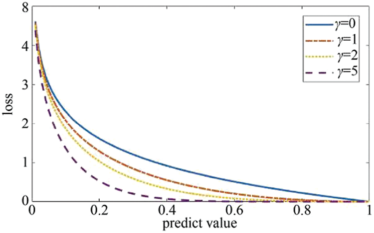
Figure 4: Loss comparison under various values of learning rate γ

fl(t,y)={−α(1−t)γlog⁡(t),y=1−αtγlog⁡(1−t),y=0(13)

During the training process of the model, when positive samples are misidentified, they will be regarded as difficult samples. At this time, there is a gap of tens or even hundreds of times between (f(xi))γ and (1−f(xi))γ, the weight of difficult samples can be increased to improve the classification performance of nnPU under data imbalance. The modified non-negative risk estimator is shown in formula (14).

R¯(fl)=πEP(fl(f(x),1))+max(0,EU(l(f(x),0))−πEP(fl(f(x),0)))(14)

The specific steps of positive unlabeled learning are shown in Algorithm 3.

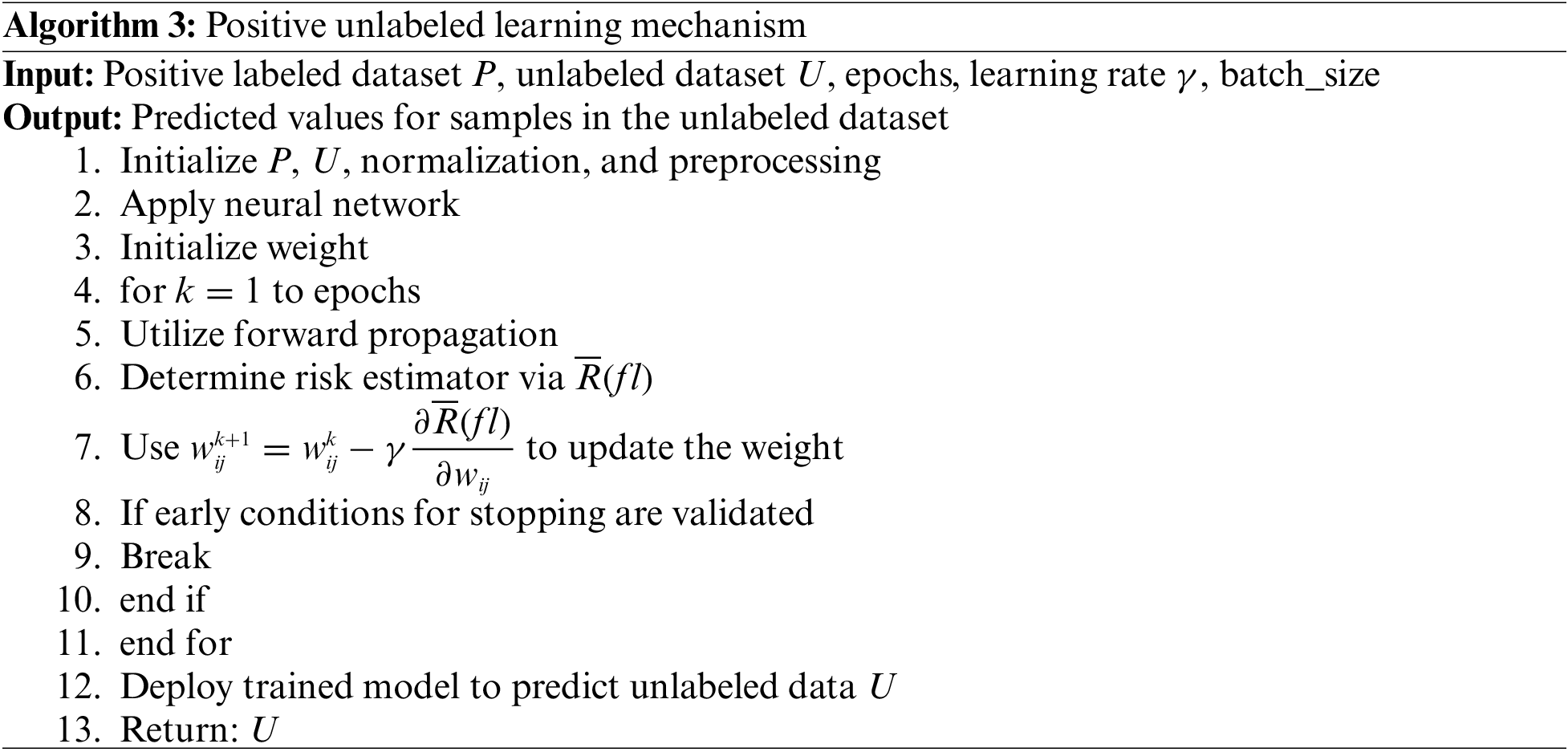
From the above analysis, it can be seen that compared with the binary classification model, positive unlabeled learning is adjusted in the error calculation, the binary classification error is estimated through the risk estimator, and the estimated binary classification error is used for backpropagation to adjust the parameters of the neural network model.

3.3.2 Neural Network Settings

In the process of using machine learning methods for industrial control system intrusion detection, it is necessary to pay attention to the real-time requirements of the industrial control system for the model, and the model is required to quickly make judgments on the input data. Therefore, the neural network structure used needs to be simplified as much as possible. On the one hand, the simplified model can reduce the detection response time and improve the real-time performance of the model. On the other hand, it can reduce the demand for computing resources and is more in line with the application scenarios of industrial control systems.

Positive unlabeled learning is a learning algorithm based on neural networks, which trains neural network models by estimating classification errors in scenarios where there is only one type of labeled data. The difference in neural network structure will also affect the performance of the model. In this section, we discuss two positive unlabeled learning models with different network structures.

The first is a fully connected deep neural network (DNN). It is a neural network with multiple hidden layers. In theory, DNN can fit any function. Reference [42] discussed the classification performance of DNN with different numbers of hidden layers in intrusion detection, and the results show that when performing binary classification, the DNN model with three hidden layers can have relatively high classification performance, and as the number of layers increases, the classification performance does not improve significantly. Therefore, in this paper, a DNN model with 3 hidden layers is selected, and the numbers of the three hidden nodes are 256, 64, and 16, respectively. The network structure settings of the model are shown in Table 4.

The positive unlabeled learning completes a binary classification task through DNN, divides all samples to be detected into normal traffic and intrusion traffic, and the output of DNN is mapped to the [0,1] interval through the Sigmoid function to complete the binary classification task.

In DNN, batch normalization (BN) is performed between two fully connected layers, that is, the output of each hidden layer neuron is standardized, so that the input value of the nonlinear transformation function falls into an area that is more sensitive to the input. The use of BN can speed up the convergence of the neural network. In addition, BN allows the model to use a higher learning rate and reduces the model’s requirements for network parameter initialization. It can also act as a regulator, and in some cases can eliminate the need for dropout.

The activation function in DNN is the ReLu function. (1) It can speed up network training. Compared with sigmoid and tanh, its derivation is faster. (2) Prevent the gradient from disappearing. When the value is too large or too small, the derivatives of sigmoid and tanh are close to 0, and ReLu is an unsaturated activation function, which does not exist. (3) Make the grid sparse.

The weight update algorithm uses the Adam algorithm, which is an adaptive learning rate optimization algorithm, and has the advantages of fast convergence and less memory usage.

The second is the Convolutional Neural Network (CNN). In this paper, a simple CNN network structure Lenet-5 structure is adopted. Considering that Lenet-5 is a network for processing two-dimensional images, the input is required to be 32 × 32, and the data of industrial control systems are usually one-dimensional vectors, so the network structure is adjusted to replace the two-dimensional convolution in Lenet-5 as For one-dimensional convolution, the input size is 32 × 1. Therefore, it is necessary to perform feature selection and reduce the dimension to 32 dimensions before training the model. The first layer of the network uses a 5 × 1 convolution, and after passing through the first layer, six feature maps with a size of 28 × 1 are obtained, and then through the maximum pooling sampling with a size of 2, the size is changed to 14 × 1. The first convolutional layer uses 5 × 1 convolution to output 16 feature maps with a size of 10 × 1, and then changes it to 5 × 1 through the maximum pooling sampling with a size of 2, and finally flattens all images into a fully connected layer, the fully connected layer has two layers, the number of neurons in the first layer is 120, and the number of neurons in the second layer is 84. Finally, according to the classification category, the output is performed through the softmax function. The model structure of the industrial control system based on Lenet-5 is shown in Fig. 5. The “?” in the input (?, 32, 1) represents the batch size, and the activation function uses the ReLu function.

Figure 5: CNN-based framework for intrusion detection in positive unlabeled learning

So far, the model structure based on positive unlabeled learning can be obtained. The offline training steps of the intrusion detection model based on positive unlabeled learning are as follows:

•   Read data, including positive label data and unlabeled data to be detected, and perform data preprocessing;

•   Using the OCSVM-cE technique, estimate the class prior probability of the unlabeled data set and save the OCSVM model;

•   Calculate the feature importance through the KL divergence, set the threshold th or the selected feature number K, and perform feature selection according to the feature importance to obtain a new training data set;

•   Initialize a deep neural network and use the new training data set after feature selection to train the PU learning model. The training process is shown in Algorithm 3;

•   Export the trained neural network and return the predicted value of the unlabeled dataset.

4  Experimental Results

4.1 Data Introduction and Analysis

Three publicly available datasets for intrusion detection are used in the experiments: NSL-KDD [43], UNSW-NB15 [44], and WADI [45]. Among them, the data in the NSL-KDD and UNSW-NB15 datasets are based on the characteristics extracted from Internet traffic, including the basic characteristics of the flow (such as transport layer protocol type, port, etc.), time information of the flow, connection content characteristics, etc. These characteristics can also be provided as industrial control system traffic. At the same time, to further verify the effectiveness of the model in the industrial control scene, the WADI dataset is introduced. On the one hand, the industrial control data provided by the industrial control test bench is applied to the data. On the other hand, simulates the unbalanced characteristics of industrial control data.

In terms of attack types, the NSL-KDD dataset is improved on the KDDCUP99 dataset, and some redundant data are removed. The dataset contains normal traffic and 22 types of attack traffic. The attack traffic mainly includes denial of service attack (DoS), monitoring and detection (Probing), remote machine illegal access (R2L), and ordinary user unauthorized access (U2R) four categories. The UNSW_NB15 dataset is an intrusion detection dataset generated by the Australian Cyber Security Center, including samples of 9 types of attacks including DoS and Backdoors. The WADI dataset is collected on an attached test rig, which consists of many large tanks that supply water to user tanks. The WADI dataset contains 16 attacks whose goal is to stop the water supply to the user tanks.

In the experiment, the UNSW-NB15 dataset uses the training and testing data sets provided by the official website, with a total of 257,673 samples. The WADI dataset uses labeled data from October 2019. The sample size of each data set is shown in Table 5.

4.2 Data Preprocessing

In the division of training and test data sets, based on the true labels of the samples, a specified number of positive samples are randomly selected from the positive data as the training set, and the remaining data are used as the test set. In terms of data processing, for the string data existing in NSL-KDD, such as protocol types and services, one-hot encoding is required to convert the string into a vector, and the dimension of the NSL-KDD dataset after encoding is increased from 41 dimensions to 122 dimensions. The data in the UNSW-NB15 and WADI datasets do not have null values and strings, so they can be used directly.

The equipment used in this experiment: the processor is Intel core i7 8750H, the operating system is 64-bit Windows 10 Home Chinese Edition, the hard disk is Western Digital SN720, and the memory is 16 GB.

4.3 Evaluation Index

After the model is trained, the data set to be predicted is classified through the model, and based on the judgment result of the model, the confusion matrix shown in Table 6 can be established.

As shown in Tables 2–5, the row represents the true category of the data, and the column represents the predicted category of the model. In intrusion detection, the focus is on the ability of the model to identify intrusion samples. Therefore, the precision and recall of intrusion samples are used as evaluation indicators. In the sample, the true label is the proportion of positive examples, as shown in formula (15).

precision=TPTP+FP(15)

The recall rate is shown in formula (16). The recall rate describes the proportion of the model that recognizes all samples of the true category as positive examples.

recall=TPTP+FN(16)

The F1-score is also often used as an evaluation index. F1-score is the harmonic mean of precision and recall, as shown in the formula (17).

F1=21precision+1recall=2×precision×recallprecision+recall(17)

In addition to the above indicators, in the intrusion detection scenario, due to the large amount of data faced, the time taken for model training and prediction is also an important indicator to measure the performance of the model.

4.4 Analysis of Results

4.4.1 Effectiveness Analysis and Time Efficiency of Feature Importance

In this experiment, the importance of each feature is first calculated by random forest in the binary classification scenario, and compared with the feature importance calculated based on KL divergence to verify the effectiveness of the feature weight calculated using KL divergence.

In the experiment, 2000 positive samples were randomly selected from all samples as the positive label data set, and then 2000 positive samples and 4000 negative samples were mixed as the unlabeled data set, and all the remaining samples were used as the test set. Figs. 6 and 7 show the experimental results of the KLOCSVM and KDE-OCSVM algorithms in the NSL-KDD dataset and the UNSW-NB15 dataset, respectively.

Figure 6: Evaluation of feature importance (UNSW-NB15)

Figure 7: Evaluation of feature importance (NSL-KDD)

Further, the correlation of the feature importance obtained by the two algorithms is calculated and the correlation test is carried out. By calculation, under the UNSW-NB15 data set, the average correlation coefficient of the feature importance of the two algorithms after normalization is 0.72, and the p value of the test is 4.29 ×10–7. The correlation coefficient on the NSL-KDD data set is 0.9364, and the p value of the test is 1.15 ×10–56. With a significance level of 0.05, it can be concluded that there is a significant correlation between the feature importance calculated by KL divergence and the feature importance in the case of binary classification, that is, the feature importance calculated by KL divergence is effective.

4.4.2 Class Prior Probability Estimation

To verify the effectiveness of the OCSVM-cE algorithm proposed in this paper, it is compared with the following class prior probability algorithm.

•   KM1/KM2 algorithm. This algorithm embeds it into the kernel space by calculating the distribution of positive and negative data sets and can solve the class prior probability by solving a quadratic programming problem. The algorithm is an algorithm with high estimation accuracy at present.

•   TICE algorithm. This algorithm divides all samples based on a decision tree, raises the lower bound of the label frequency of positive samples through subsets, obtains the estimated value of the label frequency of positive samples, and then calculates the class priority. This algorithm is currently the algorithm with the lowest time complexity for class-prior probability estimation.

•   One-class SVM-cE algorithm. The algorithm proposed in this paper trains the One-class SVM model to find reliable positive examples of unlabeled datasets, estimates the label frequency of positive examples through the reliable positive examples, and then calculates the class prior probability.

In the class prior probability estimation problem, the core evaluation index is the estimation accuracy, that is, the error between the estimated value and the real value. In addition, the time complexity of the algorithm is also an important evaluation index.

Based on the above evaluation indicators, the following two experiments are designed for verification: 1) To verify the accuracy of class prior probability estimation, construct unlabeled data sets with different class prior probabilities in the experiment, and estimate the class prior probabilities of the constructed unlabeled data sets through four different baseline algorithms, analyze the error between the estimated value of different algorithms and the real value; 2) Verify the time complexity of the algorithm. In this experiment, we first compare the time required for each algorithm to estimate the class prior probability under the same sample size, and then estimate the time trend of the class prior probability under different sample sizes.

The first is the accuracy of class prior probability estimates. In the experiment, the sample size of the positive label dataset is set to 1000, and the number of negative samples in the unlabeled dataset is 2000, respectively, constructing unlabeled datasets with class prior probabilities of 0.1, 0.2, 0.3, 0.4, and 0.5. The class prior probabilities were estimated for the constructed datasets using baseline algorithms, respectively.

The experimental results are shown in Figs. 8 and 9. The abscissa is the prior probability of the real class, and the ordinate is the absolute value of the error between the estimated value and the predicted value. The experimental results show that the one-class SVM-cE algorithm can maintain high prediction accuracy on the two data sets, the error is close to that of the KM2 algorithm and maintained below 0.05, and the stability of the algorithm estimation is better.

Figure 8: Error comparison of algorithms (UNSW-NB15)

Figure 9: Error comparison of algorithms (NSL-KDD)

During the experiment, the TIcE algorithm has a large positive error. This is because the TIcE algorithm estimates the real label frequency by seeking the lower bound of the label frequency, which will cause the estimated label frequency to be lower than the real value, so the estimated class prior probability is larger than the true value. In the one-class SVM-cE algorithm, the one-class SVM algorithm is used to find reliable positive examples, avoiding the use of lower bounds, and improving the accuracy of estimation.

To further test the stability of the one-class SVM-cE algorithm estimation, the number of samples in the positive label data set is set to 2000, and the value is randomly selected in the interval [0.1,0.9] as the class prior probability to construct the unlabeled data set, and the experiment is repeated 100 times, computes the error between the class prior probability estimate and the true value.

Fig. 10 shows the boxplot of 100 repeated experiments. It can be found that the predicted effect of the one-class SVM-cE algorithm on the KDD and UNSW-NB15 data sets is better than that on the WADI data set, and the estimated four-point error is less than 0.05, while The lower quartile of the estimated error on the WADI dataset is 0.0407, the median is 0.0672, and the upper quartile is 0.0884. There are only two outliers, so the estimated value of WADI is relatively stable, and the error is concentrated in [0.05,01] interval, the estimation results of the three data sets are combined, and OCSVM-cE is a stable class prior probability estimation algorithm.

Figure 10: Error comparison of various datasets

Fig. 10 shows the boxplot of 100 repeated experiments. It can be found that the predicted effect of the one-class SVM-cE algorithm on the KDD and UNSW-NB15 datasets is better than that on the WADI dataset, and the estimated four-point error is less than 0.05, while the lower quartile of the estimated error on the WADI dataset is 0.0407, the median is 0.0672, and the upper quartile is 0.0884. There are only two outliers, so the estimated value of WADI is relatively stable, and the error is concentrated in [0.05,01] interval, the estimation results of the three datasets are combined, and one-class SVM-cE is a stable class prior probability estimation algorithm.

In PU learning, class prior probability is important prior knowledge, and its estimated error will directly affect the performance of the trained model. Through experiments, we further explore the influence of class prior probability estimation error on model performance. In the experiment, the true class prior probability of the unlabeled data set is set to 0.4, and different values are taken as the estimated value of the class prior probability in the interval [0,1] with 0.05 prior probability. The results are shown in Fig. 11. It shows the experimental results of setting the number of positive label samples to 10,000 and the number of negative samples in the unlabeled dataset to 20,000 under the UNSW-NB15 dataset. The abscissa is the estimated class prior probability, and the ordinate is the F1-score. It can be observed that when the estimated class prior probability is 0.4, the F1-score achieves its highest value, and the model’s performance is the best at this moment, and when the error between the estimated and true class prior probabilities increases. When the estimated value is zero, all unlabeled samples are classed as negative, and when the projected value is one, all unlabeled samples are classified as positive. The estimated class prior probability error from the F1-score analysis should be less than 0.05 to guarantee that the model has satisfactory classification performance.

Figure 11: F1-score evaluation under class prior

Fig. 12 shows that when the number of fixed positive samples is 1000, the time required by the one-class SVM-cE algorithm and the TIcE algorithm is positively correlated with the number of unlabeled samples [46,47]. Considering that in one-class SVM-cE, only positive samples are needed to train the OCSVM model, it can be considered that the one-class SVM-cE algorithm is more suitable for intrusion detection application scenarios, and the one-class SVM model trained in the process can be reused. When the class prior probability estimation is performed on the labeled dataset, the model can be directly loaded to classify reliable positive examples.

Figure 12: Comparison of estimation time of the algorithms (UNSW-NB15)

Fig. 13 compares the runtime of the proposed algorithm under IEC 60870-5104 [48] and DNP3 [49] datasets. As can be seen from Fig. 13, the runtime of the proposed algorithm under the IEC dataset is better than DNP3.

Figure 13: Comparison of estimation time of the proposed algorithm under IEC 60870-5104 and DNP3 datasets

4.4.3 Positive Unlabeled Learning Performance Analysis

The neural network settings of the compared binary classification model: the DNN settings are the same as the DNN network model used for PU learning. The model contains three hidden layers. The number of neurons in the first layer is 256, the number of neurons in the second layer is 64, and the number of neurons in the third layer is 16, but the positive and negative samples with real labels are used for training during the training process. The network structure of CNN uses the same LeNet-5 structure. The input is an image of 32 × 32, and the first layer uses a convolution of 5 × 5 [50]. After passing through the first layer, six images with a size of 28 × 28 feature map, and through the maximum pooling sampling of 2 × 2, it is changed to a size of 14 × 14, and the second convolutional layer uses convolution of 5 × 5 to output 16 feature maps with a size of 10 × 10, and then passes The maximum pooling sampling of 2 × 2 is changed to 5 × 5, and finally all the images are flattened and input into a fully connected layer, the number of neurons in the first layer is 120, and the number of neurons in the second layer is 84, and finally according to the classification category, output through the softmax function. RNN sets the number of hidden layer nodes to 80.

In the experiment, the number of positive labeled samples is set to 10,000, the number of negative examples in the unlabeled data set is 2000, the class prior probability is 0.9, the learning rate is 0.01, and the number of iterations is 50.

Table 7 shows the comparison results of positive unlabeled learning and binary classification models. The comparison experiments in the table can be divided into two categories: positive unlabeled learning and binary classification performance comparison under the same network structure (DNN/CNN), positive unlabeled learning, and current better performance binary classification model comparison. According to the experimental data, the precision of positive unlabeled learning under the same network topology is comparable to that of the binary classification model, however, there is little difference in the recall rate [51]. According to the previous analysis, industrial control intrusion detection requires higher precision of the model, it is expected to achieve “prefer false negatives rather than false positives”, so positive unlabeled learning is suitable for industrial control intrusion detection, and compared with the current advanced CNN-BiLSTM and other models, it can still maintain a small gap in precision. At the same time, the positive unlabeled learning compares the binary classification model, which reduces the requirements for training data. Only one type of labeled data is needed, which can effectively reduce the data collection work. At the same time, only positive and unlabeled data are used for training, so that the model can mine unknown types of intrusion.

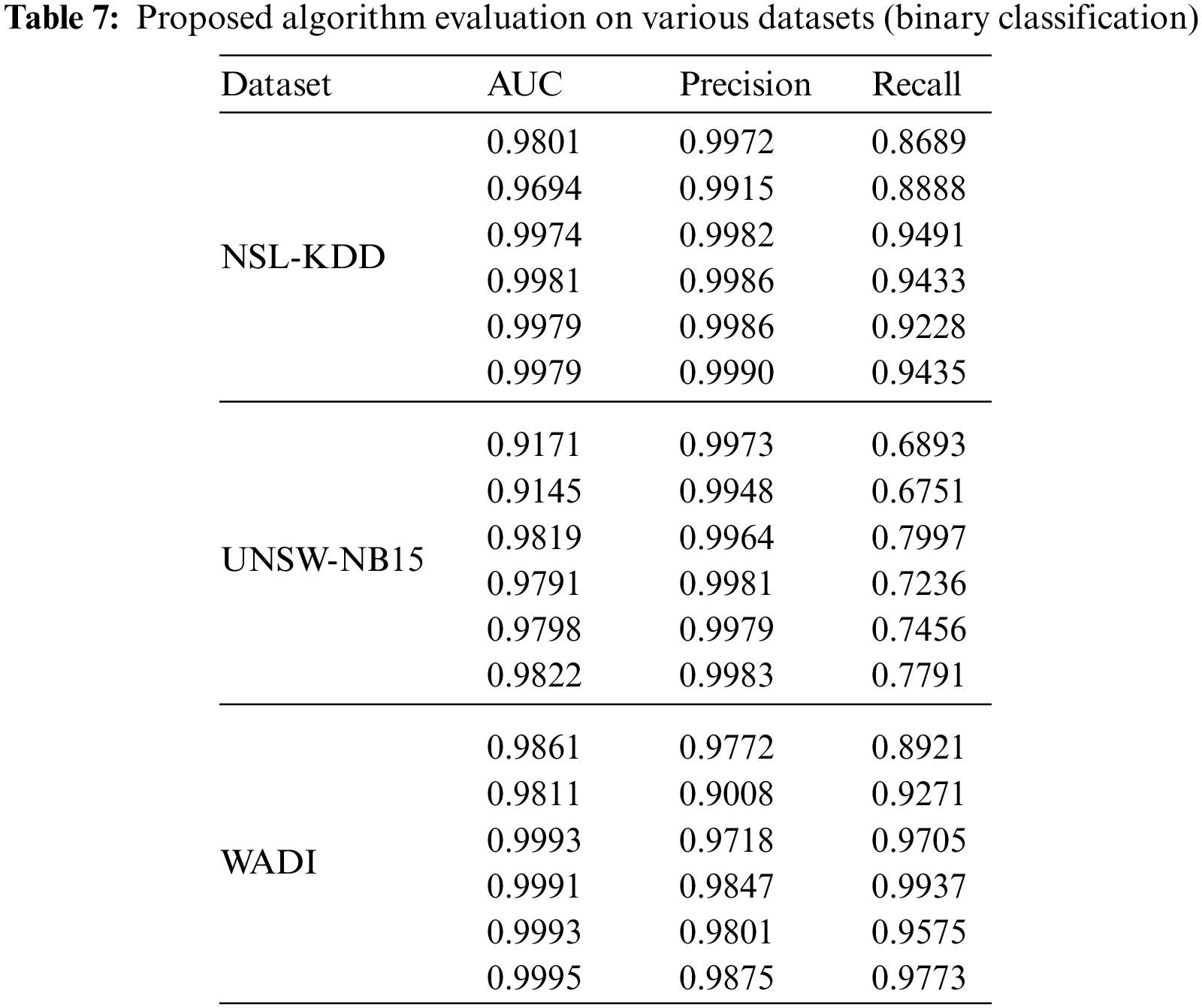
In Table 7, the experiment compares the performance of PU learning and binary classification model, then compares the proposed learning and anomaly detection model, and analyzes the performance difference under the same condition of only one type of label data. From the research analysis listed in Table 2, the anomaly detection models currently used for intrusion detection are mainly AE and one-class SVM, where AE is an unsupervised model, and consists of two parts: Encoder and decoder. The role of the encoder is to find the compressed representation of the given data. The decoder is used to reconstruct the original input and perform anomaly detection by calculating the error between the reconstructed input and the original input [52]. At the same time, looking at the research of one-class SVM for intrusion detection, its main work is focused on feature engineering. In this experiment, feature selection is based on the feature importance metric of positive unlabeled learning, and one-class SVM is used for anomaly detection. In terms of parameter setting, one-class SVM sets the upper limit of the error to 0.1, and the parameters of AE adopt the default settings in the source code.

Table 8 shows the comparison results of the positive unlabeled learning and anomaly detection models. The indicators in the table show that, in particular, it can be observed that the performance of the one-class SVM and AE models on the WADI dataset is poor, which is caused by the imbalance of the test data. The ratio of positive data to negative data in the test data set is about 16:1, which also shows that the one-class SVM and AE algorithms are insufficient when dealing with unbalanced data, and positive unlabeled learning improves the performance of the model under unbalanced data through focal loss [53]. Therefore, positive unlabeled learning has significantly improved the precision rate and recall rate. On the three data sets, the proposed algorithm has significantly better performance than AE and one-class SVM in terms of precision rate.

Combining the results of Tables 7 and 8, it is not difficult to find that although proposed learning is similar to the anomaly detection algorithm in terms of training data, only one type of label data is needed, but the classification performance of the trained model has a larger gap than that of the anomaly detection algorithm. Especially in industrial control scenarios, taking the WADI dataset as an example, the ratio of normal data to abnormal data is as high as 16:1, and proposed learning can also maintain a high precision and recall rate, compared with some binary classification algorithms, their only a slight difference in precision. Combined with the previous characteristics of industrial control scenarios, the proposed learning is suitable for anomaly detection in industrial control scenarios.

To sum up, this paper proposes to use proposed learning for intrusion detection. It is an algorithm similar to anomaly detection, but it needs to label positive data on the training data, and the positive data needs to meet the SCAR condition. It can provide intrusion detection with high precision and high recall, and its precision and recall are significantly improved compared with unsupervised anomaly detection models. In particular, it is close to the binary classification model in terms of precision.

5  Conclusion

Industrial control systems are mostly utilized in nuclear power, water conservation, and other critical infrastructures. It is important to assure the safety of industrial control systems. The intrusion detection system ensures network security and is an important component of industrial control system security. In this study, a positive unlabeled learning for intrusion detection in industrial control systems and used normal traffic as label data to find aberrant samples in the data. A feature significance calculation approach for feature selection with the goals of high dimensionality and strong correlation of industrial control system data is deployed. Simultaneously, the class prior probability estimation algorithm is enhanced, and the one-class SVM-cE algorithm for class prior probability estimation is employed, which increases the estimate’s stability and accuracy. Finally, experiments are performed to validate the efficiency of the suggested learning. When compared to a supervised binary classification model, the proposed learning model maintains a high accuracy rate while having a slightly lower recall rate. Although the suggested learning approach avoids using negative data, it also imposes limits on positive data: positive samples are picked randomly. That is, their distribution is the same as the distribution of positive samples in unlabeled dataset. It is also a shortcoming of the suggested learning, and future research can concentrate on executing positive unlabeled learning on a data set with selection bias.

Acknowledgement: This research is supported by the University of Ha’il -Saudi Arabia.

Funding Statement: This research has been funded by the Research Deanship at the University of Ha’il -Saudi Arabia through Project Number RG-20146.

Author Contributions: The authors confirm their contribution to the paper as follows: study conception and design: A. Alkhalil, D. Uliyan; data collection: M. Altameemi; analysis and interpretation of results: A. Abdelrhman, Y. Altameemi; draft manuscript preparation: A. Ahmad, R. Mansour, A. Alkhalil. All authors reviewed the results and approved the final version of the manuscript.

Availability of Data and Materials: The data used for the findings of this study is available within this article.

Conflicts of Interest: The authors declare that they have no conflicts of interest to report regarding the present study.

References

1. O. Pospisil, P. Blazek, K. Kuchar, R. Fujdiak and J. Misurec, “Application perspective on cybersecurity testbed for industrial control systems,” Sensors, vol. 21, no. 23, pp. 1–24, 2021. [Google Scholar]

2. J. Hajda, R. Jakuszewski and S. Ogonowski, “Security challenges in industry 4.0 PLC systems,” Applied Sciences, vol. 11, no. 21, pp. 1–20, 2021. [Google Scholar]

3. A. Hocky, “Uncovering the cyber security challenges in healthcare,” Network Security, vol. 20, no. 4, pp. 18–19, 2020. [Google Scholar]

4. P. Radanliev and D. Roure, “Advancing the cybersecurity of the healthcare system with self-optimizing and self-adaptive artificial intelligence (part 2),” Health and Technology, vol. 12, no. 3, pp. 923–929, 2022. [Google Scholar] [PubMed]

5. S. Pal and Z. Jadidi, “Analysis of security issues and countermeasures for the industrial Internet of Things,” Applied Sciences, vol. 11, no. 20, pp. 1–19, 2021. [Google Scholar]

6. L. Wu, W. Zhang and W. Zhao, “Privacy-preserving data aggregation for smart grid with user anonymity and designated recipients,” Symmetry, vol. 15, no. 5, pp. 1–18, 2022. [Google Scholar]

7. M. Sun, Y. Lai, Y. Wang, J. Liu, B. Mao et al., “Intrusion detection system based on in-depth understandings of industrial control logic,” IEEE Transactions on Industrial Informatics, vol. 1, no. 3, pp. 1–12, 2022. [Google Scholar]

8. S. Mubarak, M. Habaebi, M. Islam, F. Rahman and M. Tahir, “Anomaly detection in ICS datasets with machine learning algorithms,” Computer Systems Science and Engineering, vol. 37, no. 1, pp. 33–46, 2021. [Google Scholar]

9. Y. Chu, Y. Lai and J. Liu, “Industrial control intrusion detection approach based on multiclassification GoogLeNet-LSTM model,” Security and Communication Networks, vol. 19, no. 1, pp. 1–10, 2019. [Google Scholar]

10. I. Butun, I. Ra and R. Sankar, “An intrusion detection system based on multi-level clustering for hierarchical wireless sensor networks,” Sensors, vol. 15, no. 11, pp. 1–19, 2015. [Google Scholar]

11. H. Wang, H. Zhou, Z. Hao, S. Hu, J. Li et al., “Network traffic analysis over clustering-based collective anomaly detection,” Computer Networks, vol. 205, no. 3, pp. 1087–1098, 2022. [Google Scholar]

12. X. Duan, Y. Fu and K. Wang, “Network traffic anomaly detection method based on a multi-scale residual classifier,” Computer Communications, vol. 198, no. 2, pp. 206–216, 2023. [Google Scholar]

13. X. Li, W. Chen and Q. Zhang, “Building auto-encoder intrusion detection system based on random forest feature selection,” Computers & Security, vol. 95, no. 4, pp. 943–961, 2020. [Google Scholar]

14. A. Tama, S. Lee and J. Lee, “A systematic mapping study and empirical comparison of data-driven intrusion detection techniques in industrial control networks,” Archives of Computational Methods in Engineering, vol. 29, no. 5, pp. 5353–5380, 2022. [Google Scholar]

15. S. Zhang, Z. Liu, Y. Jia, J. Ren and X. Zhao, “Network intrusion detection method based on PCA and Bayes algorithm,” Security and Communication Networks, vol. 18, no. 4, pp. 1–10, 2018. [Google Scholar]

16. O. Tushkanova, D. Levshun, A. Branitskiy, E. Fedorchenko, E. Novikova et al., “Detection of cyberattacks and anomalies in cyber-physical systems: Approaches, data sources evaluation,” Algorithms, vol. 16, no. 2, pp. 1–17, 2023. [Google Scholar]

17. J. Ling, Z. Zhu, Y. Luo and H. Wang, “An intrusion detection method for industrial control systems based on bidirectional simple recurrent unit,” Computers & Electrical Engineering, vol. 91, no. 5, pp. 7049–7063, 2021. [Google Scholar]

18. S. Huda, Y. Yearwood and M. Hassan, “Securing the operations in SCADA-IoT platform based industrial control system using an ensemble of deep belief networks,” Applied Soft Computing, vol. 71, no. 1, pp. 66–77, 2018. [Google Scholar]

19. J. Nedeljkovic and Z. Jakovljevic, “CNN-based method for the development of cyber-attacks detection algorithms in industrial control systems,” Computers & Security, vol. 114, no. 3, pp. 2585–2598, 2022. [Google Scholar]

20. N. Ahmed, V. Krishan and S. Foroutan, “Cyber-physical security analysis for anomalies in transmission protection systems,” IEEE Transactions on Industry Applications, vol. 55, no. 6, pp. 6313–6323, 2019. [Google Scholar]

21. Z. Wang, Y. Lai, Z. Liu and J. Liu, “Explaining the attributes of a deep learning based intrusion detection system for industrial control networks,” Sensors, vol. 20, no. 14, pp. 1–23, 2020. [Google Scholar]

22. S. Li, J. Yang and J. Wu, “Web intrusion detection system combined with feature analysis and SVM optimization,” EURASIP Journal on Wireless Communications and Networking, vol. 33, no. 1, pp. 1–18, 2020. [Google Scholar]

23. S. Han, Q. Wu and Y. Yang, “Machine learning for internet of things anomaly detection under low-quality data,” International Journal of Distributed Sensor Networks, vol. 18, no. 10, pp. 717–731, 2022. [Google Scholar]

24. A. Khan, D. Pi and Z. Khan, “HML-IDS: A hybrid-multilevel anomaly prediction approach for intrusion detection in SCADA systems,” IEEE Access, vol. 7, no. 5, pp. 89507–89521, 2019. [Google Scholar]

25. Z. Liu, C. Wang and W. Wang, “Online cyber-attack detection in the industrial control system: A deep reinforcement learning approach,” Mathematical Problems in Engineering, vol. 22, no. 7, pp. 1–8, 2022. [Google Scholar]

26. L. Xu, K. Xu, Y. Qin, Y. Li and X. Huang, “TGAN-AD: Transformer-based GAN for anomaly detection of time series data,” Applied Sciences, vol. 12, no. 16, pp. 1–15, 2022. [Google Scholar]

27. S. Priyanga and K. Krithivasan, “Detection of cyberattacks in industrial control systems using enhanced principle component analysis and hypergraph-based convolution neural network (EPCA-HG-CNN),” IEEE Transactions on Industry Applications, vol. 56, no. 4, pp. 4394–4404, 2020. [Google Scholar]

28. F. Ayo, S. Folorunso, A. Alli, A. Adekunle and J. Awotunde, “Network intrusion detection based on deep learning model optimized with rule-based hybrid feature selection,” Information Security Journal: A Global Perspective, vol. 29, no. 6, pp. 267–283, 2020. [Google Scholar]

29. L. Zhu, S. He, L. Wang, W. Zeng and J. Yang, “Feature selection using an improved gravitational search algorithm,” IEEE Access, vol. 7, no. 3, pp. 114440–114448, 2019. [Google Scholar]

30. L. Lv, W. Wang, Z. Zhang and X. Liu, “A novel intrusion detection system based on an optimal hybrid kernel extreme learning machine,” Knowledge-Based Systems, vol. 195, no. 4, pp. 648–661, 2020. [Google Scholar]

31. Q. Zhang, V. Wild, S. Filippi, S. Flaxman and D. Sejdinovic, “Bayesian kernel two-sample testing,” Journal of Computational and Graphical Statistics, vol. 31, no. 4, pp. 1164–1176, 2022. [Google Scholar]

32. A. Scott, “A rate of convergence for mixture proportion estimation, with application to learning from noisy labels,” Artificial Intelligence and Statistics, vol. 15, no. 3, pp. 838–846, 2015. [Google Scholar]

33. M. Plessis and M. Sugiyama, “Semi-supervised learning of class balance under class-prior change by distribution matching,” Neural Networks, vol. 50, no. 3, pp. 110–119, 2014. [Google Scholar] [PubMed]

34. M. Plessis and M. Sugiyama, “Class prior estimation from positive and unlabeled data,” IEICE Transactions on Information and Systems, vol. 97, no. 5, pp. 1358–1362, 2014. [Google Scholar]

35. M. Plessis, G. Niu and M. Sugiyama, “Class-prior estimation for learning from positive and unlabeled data,” Machine Learning, vol. 106, no. 4, pp. 463–492, 2017. [Google Scholar]

36. M. Lazecka, J. Mielniczuk and P. Teisseyre, “Estimating the class prior for positive and unlabeled data via logistic regression,” Advances in Data Analytics and Classification, vol. 15, no. 1, pp. 1039–1068, 2021. [Google Scholar]

37. M. Plessis, G. Niu and M. Sugiyama, “Analysis of learning from positive and unlabeled data,” Advances in Neural Information Processing Systems, vol. 7, no. 2, pp. 703–711, 2014. [Google Scholar]

38. H. Bao, T. Sakai, I. Sato and M. Sugiyama, “Convex formulation of multiple instances learning from positive and unlabeled bags,” Neural Networks, vol. 105, no. 7, pp. 132–141, 2018. [Google Scholar] [PubMed]

39. A. Wolf, S. Regnery, R. Tarnawski, B. Billewicz, J. Polanska et al., “Weakly supervised learning with positive and unlabeled data for automatic brain tumor segmentation,” Applied Sciences, vol. 12, no. 21, pp. 1–18, 2022. [Google Scholar]

40. L. Zhang, F. Zhu, X. Ling and Q. Liu, “Best-in-class imitation: Non-negative positive-unlabeled imitation learning from imperfect demonstrations,” Information Sciences, vol. 601, no. 2, pp. 71–89, 2022. [Google Scholar]

41. J. Bekker and J. Davis, “Learning from positive and unlabeled data: A survey,” Machine Learning, vol. 109, no. 4, pp. 719–760, 2020. [Google Scholar]

42. Y. Kim and P. Panda, “Revisiting batch normalization for training low-latency deep spiking neural networks from scratch,” Frontiers in Neuroscience, vol. 15, no. 4, pp. 1–13, 2021. [Google Scholar]

43. Y. Tang, L. Gu and L. Wang, “Deep stacking network for intrusion detection,” Sensors, vol. 22, no. 1, pp. 1–18, 2022. [Google Scholar]

44. N. Moustafa and J. Slay, “UNSW-NB15: A comprehensive data set for network intrusion detection systems (UNSW-NB15 network data set),” in Conf. Military Communications and Information Systems (MilCIS), Sydney, Australia, pp. 1–6, 2015. [Google Scholar]

45. M. Ahmed, V. Palleti and A. Mathur, “WADI: A water distribution testbed for research in the design of secure cyber-physical systems,” in IEEE 3rd Int. Workshop on Cyber-Physical Systems for Smart Water Networks, New York, USA, pp. 25–28, 2017. [Google Scholar]

46. W. Lin, H. Lin and P. Wang, “Using convolutional neural networks to network intrusion detection for cyber threats,” in IEEE Int. Conf. on Applied System Invention, Seoul, South Korea, pp. 1107–1110, 2018. [Google Scholar]

47. L. Yin, Y. Zhu and J. Fei, “A deep learning approach for intrusion detection using recurrent neural networks,” IEEE Access, vol. 5, no. 3, pp. 21954–21961, 2017. [Google Scholar]

48. IEC 60870-5-104 Intrusion Detection Dataset. [Online]. Available: https://zenodo.org/record/7108614 [Google Scholar]

49. DNP3 Intrusion Detection Dataset. [Online]. Available: https://zenodo.org/record/7348493 [Google Scholar]

50. https://standards.ieee.org/ieee/C37.118.1/4902/ [Google Scholar]

51. https://iec61850.dvl.iec.ch/ [Google Scholar]

52. https://www.dnp.org/About/Overview-of-DNP3-Protocol [Google Scholar]

53. https://www.ipcomm.de/protocol/IEC104/en/sheet.html [Google Scholar]