Graph-Based Feature Learning for Cross-Project Software Defect Prediction

1  Introduction

Software defect prediction (SDP) is a challenging task in software engineering that aims to identify potential defects in software systems early during software development. Defect prediction aims to help software developers and testers prioritize their efforts and resources toward the most likely problematic areas of the software codebase, ultimately improving the software quality and reliability [1–3]. Extracting features from source code is symbiotic with the software quality assurance model and helps with the software testing process. Effective feature extraction not only aids in identifying potential defects and vulnerabilities early in the development cycle and aligns with the principles of open-source software quality assurance [4–6]. By comprehensively analyzing code interdependencies, design patterns, and intricate relationships, feature extraction techniques enhance the ability to identify and rectify issues promptly, fostering higher software quality.

Early research in defect prediction focused mainly on within-project defect prediction (WPDP), where data from a single project was used to build and test predictive models in the same project. The underlying principle of this approach is that by leveraging patterns and trends within the historical data of the projects, it becomes possible to pinpoint areas of high risk within the software codebase [7,8]. One of the main advantages of WPDP is that it can be tailored to the specific characteristics and context of the project, such as the programming language, development process, and team expertise. However, WPDP can suffer from limited training data; within a single project, the available training data for defect prediction may be limited, especially for rare or severe defects [9]. This challenge can make it difficult to build accurate and reliable models. To address the issue of limited data in certain single projects, researchers employed data from well-established software projects (known as the source project) to construct an SDP model that can be applied to predict faults in another software project (referred to as the target project). This approach is the fundamental concept behind the cross-project defect prediction (CPDP) approach. The objective of CPDP is to utilize data from multiple software projects to improve the accuracy and generalizability of defect prediction models [10–12].

Most previous studies in CPDP [13–21] have used traditional static features to train machine learning algorithms for predicting potential defects. These traditional CPDP models rely on handcrafted features, such as code size, code complexity, and process features, to train machine learning models that classify code parts as defective or non-defective. Traditional features-based CPDP approaches have shown tangible success in predicting defects in new projects. However, these models often suffer from low prediction accuracy and limited generalization to new projects due to the variability in software projects and difficulty defining meaningful features for different projects.

Recently, deep learning has become increasingly popular for SDP. Some researchers have proposed CPDP models that can automatically learn semantic (syntactic) features from source code. For instance, Wang et al. [22] used a deep belief network (DBN) to extract syntactic features from Abstract Syntax Trees (ASTs) of program modules. These learned features were subsequently utilized to build the SDP model. Chen et al. [23] introduced the CPDP approach based on deep learning. They extracted a simplified AST to represent each program module in the source code. Then they used Bi-directional LSTM to learn syntactic features from simplified AST nodes. Dynamic syntactic features-based approaches can help effectively differentiate the semantics of various code snippets, a task that traditional features cannot address adequately. However, these methods often cannot capture the complex relationships among software products, such as function calls and variable dependencies. Fig. 1 shows a motivating example of a defect in a real-world Java code. The defect revolves around three methods: the “fetchProductInfo” method (Method 1) retrieves information about a product by utilizing the “getProductDetails” method (Method 3) to retrieve its details and then employs the “getDataTypeInfo” method (Method 2) to validate and process the attribute data types. This validation is crucial to find the appropriate description for the processed data node. However, the defect arises due to inconsistencies in handling the case sensitivity of the attribute names. While the attribute names within the data are lowercase (line 2, Method 2), the product identifier is not. Consequently, the validation process in Method 2 might not function correctly due to this case discrepancy. To address this defect, a fix is implemented by modifying the “getProductDetails” method (Method 3). The developer introduced a method call to convert the product identifier into lowercase (lines 2–3, Method 3) before performing the lookup in the product details map. This modification ensures consistency in handling case sensitivity and resolves the defect.

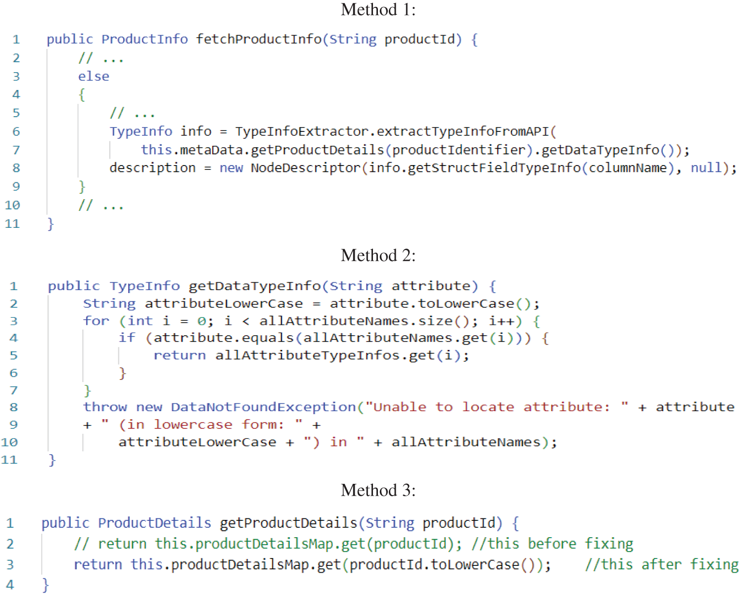
Figure 1: Motivating Java code example

Two important observations have been drawn from this example as the following:

Observation 1 (O1): This defect involves multiple methods, and to completely understand and detect this defect, it is necessary to consider the dependencies and relationships among these methods. However, existing CPDP approaches often examine code within a method individually without considering interprocedural dependencies. For example, traditional features-based CPDP [15–19] uses handcrafted features to train machine learning algorithms for predicting potential defects, and semantic features-based CPDP [22,23] uses syntactic features extracted from ASTs of program modules to train deep learning models and predict defects, cannot detect this defect because they focus on individual methods and do not consider cross-method dependencies.

Observation 2 (O2): Complex defects like the one described can have diverse paths and dependencies contributing to their emergence. A uniform weighting of paths, as seen in existing approaches, might not effectively capture these critical paths. GB-CPDP addresses this limitation by employing graph-based embeddings that consider the significance of multiple graph representations that need to be considered, such as CFGs and PDGs, allowing for more accurate defect detection by prioritizing paths that are relevant to defects.

This example is a compelling motivation for adopting the proposed GB-CPDP model. By leveraging graph-based feature learning, the model can comprehensively capture the intricate relationships and dependencies between methods, enhancing the accuracy of CPDP. This paper introduces a graph-based feature learning approach for CPDP to address these challenges. In the proposed approach, source code features are extracted and learned from CFG and DDG using NetworkX. Subsequently, an LSTM is employed to learn a predictive model based on the acquired features. Our approach consists of three main phases: (1) graph construction, where the software items are represented as a graph and extract relevant features; (2) feature learning, where LSTM is used to learn feature representations from the graph; and (3) defect prediction, where the classifier is trained to predict defective code parts based on the learned features. The prediction performance of our model is evaluated using commonly used measures in defect prediction models F1-measure and AUC. According to experimental findings on nine Java projects, our proposed GB-CPDP outperforms baseline techniques regarding F1-measure and AUC under CPDP.

The main contributions of this paper are as follows:

•   We propose a new approach for CPDP using graph-based feature learning, which can capture the complex relationships among software projects, transfer data from related source projects, and handle missing or limited data in target projects.

•   We build a defect prediction model using the LSTM for learning the extracted graph features to enhance the defect prediction performance.

•   We conduct extensive experiments on several benchmark datasets and demonstrate that our approach outperforms several baseline methods and achieves competitive results compared to the best-performing methods.

Following is a summary of the rest of this paper. Section 2 reviews the related works. Section 3 explains the proposed approach to constructing a graph, learning graph features, and then utilizing the acquired features to predict defects. The experimental setup and results analysis is presented in Section 4. Section 5 presents threats to validity. Finally, our study is summarized in Section 6.

2  Related Work

2.1 Cross-Project Software Defect Prediction (CPDP)

CPDP approaches focus on developing predictive models for detecting software defects in target projects by leveraging data from related source projects [24,25]. The CPDP models aim to transfer data learned from source projects, which possess sufficient training data and established defect patterns, to target projects that may have limited or no historical data on defects. That leads to overcoming the scarcity of labeled data in target projects and enhancing the prediction capability [26].

Over the past years, CPDP has gained significant interest from industrial and academic communities. Initially, studies [13,27] focused on exploring the feasibility of CPDP. Their findings highlighted the potential risks of utilizing data from external projects to create a predictive model for a proprietary project. Consequently, advanced transfer learning methods have been employed to enhance CPDP. Recently, scholars [18,28–30] have increasingly focused on the CPDP model. Jin [18] introduced DA-KTSVM, which is a defect prediction model created using domain adaptation (DA) incorporating kernel twin (KT) with a support vector machine (SVM). The model aimed to create two nonparallel hyperplanes, where one hyperplane was close to one class and maintained a specific distance from the other. Limsettho et al. [28] introduced a model based on estimating the distribution of classes using synthetic minorities to enhance the performance of CPDP and prevent oversampling. Their method calculated the class distribution of the desired project. Subsequently, synthetic minority over-sampling technique (SMOTE) is utilized to adjust the class distribution of the training data until it corresponds with the inverse target project distribution.

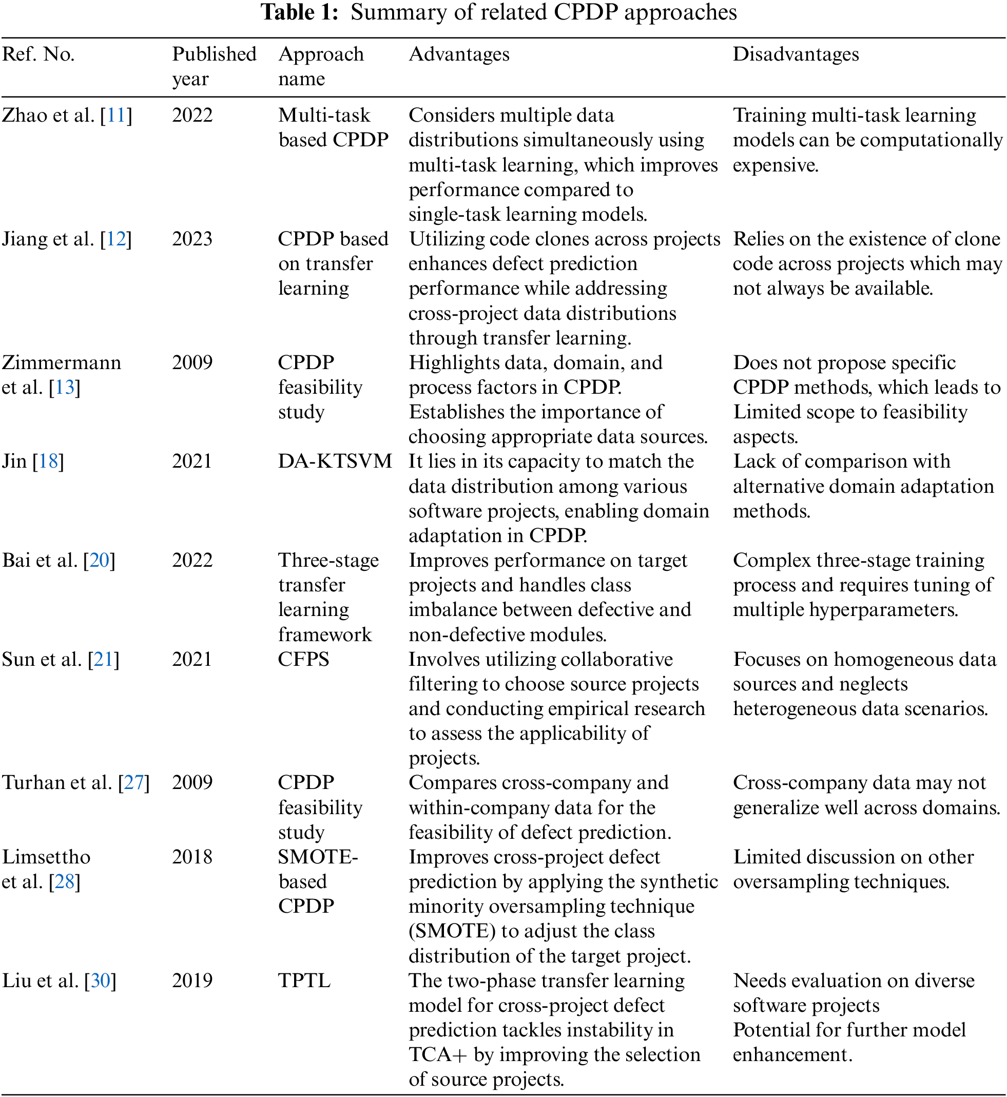
Sun et al. [21] introduced a source project selection technique termed collaborative filtering-based project source selection (CFPS). CFPS comprises three steps: inter-project similarity identification, inter-project applicability assessment, and collaborative filtering-based recommendations. Liu et al. [30] created a CPDP model involving two phases transfer learning (TPTL). During the initial phase, they suggested using a source project estimator to choose two source projects that are most similar in their distribution to a target project from a group of candidates. They prioritized the F1-score and cost-effectiveness values during this selection process. Zhao et al. [11] proposed an approach based on multiple data distribution simultaneously that improves the overall performance of CPDP. Jiang et al. [12] proposed a transfer-learning approach to predict clone consistency in software projects. The goal is to identify and predict consistent defects across clones, both at the time of creation and change. Bai et al. [20] proposed a three-stage transfer learning framework for multi-source CPDP and addressed multi-source and cross-project challenges. Table 1 introduces the summary and comparison of related works in CPDP approaches.

2.2 Long-Short-Term Memory (LSTM) in Software Defect Prediction

There has been significant research interest in applying deep learning techniques to SDP tasks in recent years. One prominent architecture that has gained attention in this field is LSTM. LSTM is a Recurrent Neural Network (RNN) type designed to deal with long-term dependencies in data [31]. This makes it particularly well-suited for modeling sequential data and capturing long-term dependencies.

The LSTM architecture consists of three main gates, as shown in Fig. 2: input, forget, and output gates. The input gate identifies the relevant input sequence elements that must be retained in the memory cell. It takes input from the current step and the previous hidden state and applies a sigmoid activation function to produce an output between 0 and 1. The role of the forget gate is to decide which data from the previous memory cell state ought to be eliminated. The output gate controls the output of the cell. It determines which memory cell information should be output to the next hidden state.

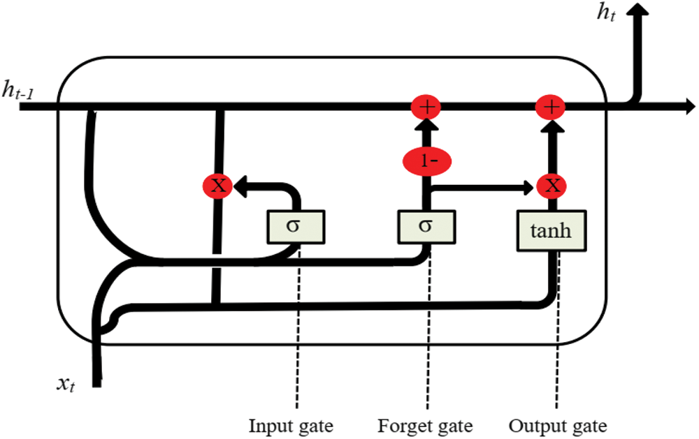
Figure 2: LSTM architecture

Several studies have used LSTM in building software defect prediction models. For example, Liang et al. [32] introduced an SDP model that combines LSTM and word embedding techniques. The method involves extracting a token sequence from the source code and mapping each token to a real-valued vector using an unsupervised word embedding model. Subsequently, they employed LSTM to acquire semantic information from programs and predict defects. Majd et al. [33] introduced SLDeep, an SDP approach that utilizes deep learning models and statement-level metrics to predict defects in software. The model was optimized using 32 metrics, including the number of operators in a given statement. LSTM was employed as the learning model for experiments conducted on 119,989 C/C++ programs, demonstrating its potential for software defect prediction. Deng et al. [34] employed an LSTM to capture contextual features from the source code. They extracted ASTs and evaluated the preservation of information for different node types. By traversing the ASTs and inputting them into the LSTM model, they successfully learned the program’s contextual features to identify defective files. This study leverages the efficiency of LSTM to learn a predictive model based on the graphs feature extracted from CFG and DDG. Our proposed model consists of three sequential steps for software defect prediction. Firstly, the graph features are extracted from CFG and DDG using Networkx. Secondly, these features are transformed into integer vectors by embedding Node2vec. Finally, the resulting integer vectors are fed into an LSTM model, enabling the prediction of software defects. This structured approach provides a systematic framework for effectively leveraging graph features, embedding techniques, and LSTM networks to enhance cross-project software defect prediction capabilities.

3  Proposed Approach

This section presents an overview of our methodology. The methodology consists of three main steps: graph construction, feature learning, and defect prediction, as shown in Fig. 3. Here is a more detailed explanation of the three steps:

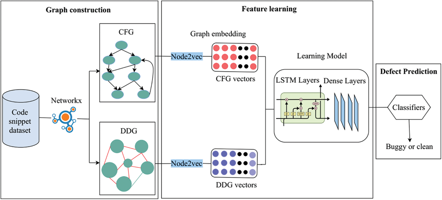
Figure 3: The architecture of the proposed model

3.1 Graph Construction

Graph construction of source code is a technique to represent the dependencies and relationships between different parts of the source code. This can be done for various purposes, such as understanding the system’s structure, identifying potential defects, or tracking changes to the system over time. In this work, the CFG and DDG are used to represent the code as a graph, analyze the code elements’ structure and dependencies, and predict the potential defects in the source code parts.

3.1.1 Control Flow Graph (CFG)

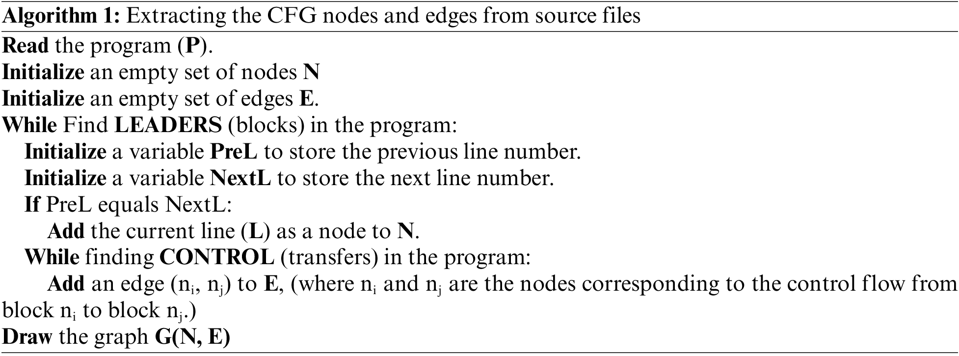
The CFG is a graphical representation of a program’s control flow or the sequence of statements and blocks. It visually represents how the program’s execution flows from one statement or block to another. The CFG helps to capture control flow within the code, analyze the program’s behavior and identify areas where errors may exist which leads to tracing the execution path, identifying unreachable code, detecting potential control flow issues like loops or conditional statements, and pinpointing potential sources of defects. The NetworkX is utilized to construct a graph G = (N, E) for each code in our dataset, where N represents a collection of nodes and E denotes a collection of edges. Each node, represented as n ∈ N, corresponds to a fundamental block within the code. Likewise, each edge, denoted as e = (ni, nj) ∈ E, symbolizes a potential control flow from block ni to block nj. Algorithm 1 illustrates extracting the nodes from the basic blocks and the edges from the control transfer statements, ensuring an accurate representation of the code’s control flow structure.

3.1.2 Data Dependence Graph (DDG)

This work aims to use every important information in the source code graph representation, which enables predict defects accurately.

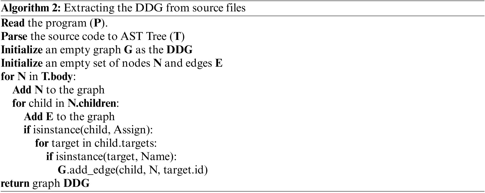
The DDG is a graphical representation that depicts the dependencies between data elements within a program. It focuses on capturing how variables or memory locations are related to each other based on the data flow between them. In a DDG, nodes represent variables or memory locations, while edges represent the data dependencies between them. DDGs are relationships between statements in which one statement’s value depends on another statement’s value. For example, if statement A assigns a value to a variable, and statement B uses that variable, then statement B is data-dependent on statement A. Algorithm 2 introduces the process of representing the DDG of the source code.

3.2 Feature Learning

This section is divided into graph embedding and the learning model. In the graph embedding part, the Node2Vec algorithm is used to embed the CFGs and DDGs into integer vectors. In the second part, the LSTM model is utilized to learn feature representations from these vectorized graphs.

3.2.1 Graph Embedding

This study leverages the power of Node2Vec, an algorithm specifically designed for graph embedding, to transform CFGs and DDGs into numerical vectors. By employing Node2Vec, the nodes in the CFGs and DDGs are represented as dense, low-dimensional vectors. Node2Vec utilizes random walks to explore the local neighborhood around each node. Then it applies the Skip-gram model to learn the vector representations based on the relationships and context within the graph. Here’s an explanation of how Node2Vec works for embedding CFGs and DDGs:

•   Random Walks: Node2Vec generates random walks on the graph to capture each node’s immediate surroundings. It simulates a random walker navigating the graph by iteratively traversing the edges. The walker can explore or exploit the neighborhood based on specific parameters such as walk length(walk_length) and walk numbers(num_walks). These random walks serve as sequences of nodes that encode the graph’s structural properties.

•   Skip-Gram Model: Once the random walks are generated, Node2Vec applies the Skip-gram model, which is a type of word embedding technique commonly used in natural language processing. The Skip-gram model learns dense vector representations for each node in the graph by predicting the context nodes given a target node.

•   Embedding Learning: The Skip-gram model learns the node embeddings by optimizing an objective function using stochastic gradient descent. It adjusts the node vectors to maximize the likelihood of predicting the context nodes accurately. This process captures the structural similarities and relationships between nodes in the graph.

•   Vector Representation: After training the Skip-gram model, each CFG node or DDG node is represented as a numerical vector, often with a fixed dimensionality. These vector representations, called node embeddings or latent representations, encode the graph’s topological and contextual information in a continuous vector space.

The vector representations are obtained using Node2Vec for nodes in CFGs and DDGs, which can then be used as inputs to LSTM.

3.2.2 Learning Model

The learning model is a crucial component of the proposed GB-CPDP and has been created using LSTM. To determine the optimal number of nodes and levels, multiple trials are conducted, which is a common practice in deep learning research. Our learning model architecture consists of eight layers, initiating with two LSTMs; each LSTM layer consists of 128 nodes. The remaining layers adhere to a standard neural network structure, with node counts of 128, 64, 32, 16, 8, and 2 for the third through eighth layers. The overall structure of our learning model is depicted in Fig. 4. As shown in Fig. 4, the input to the first LSTM layer is a sequence composed of semantic graph vectors. Except for the last layer, all dense layers utilize the ReLU as their activation function. The activation function employed in the last layer is softmax. Dropout refers to the probability of each node being excluded or dropped out.

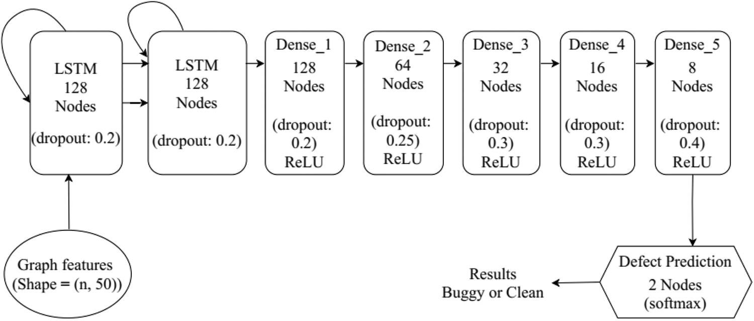
Figure 4: The overall architecture of the GB-CPDP learning model

3.3 Defect Prediction

This step is the final stage in our model, where the model can predict whether the software module is defective or clean. The final output is presented as follows:

y=softmax(W.X+b)(1)

where y represents the final output of the model, and X represents the output of the Dense_5 layer.

Softmax is the activation function applied element-wise to the output vector. It transforms the raw output values into a probability distribution over the two classes (defective or clean).

W represents the weight matrix of the softmax, and b represents the bias vector of the dense layer.

The binary_crossentropy is the chosen loss function in this stage. It evaluates the variance between the predicted and real output and quantifies the model’s performance, and it is commonly used in binary classification problems. The binary cross-entropy loss is computed using the equation:

loss(y_true,y_pred)=−(y_true*log⁡(y_pred)+(1−y_true)*log⁡(1−y_pred))(2)

where y_true represents the true labels, and y_pred represents the predicted probabilities.

The optimizer used in this model is the ‘Adam’ optimizer. Adam (Adaptive Moment Estimation) is a popular optimizer that combines the benefits of two other methods: AdaGrad and RMSProp. It efficiently adapts the learning rate based on the gradients to converge faster.

4  Experimental Setup and Results Analysis

This section provides the experimental setup and analyze the results derived from the proposed approach. The primary objective is to provide an overview of the dataset, evaluation metrics, and baseline methods. Furthermore, the results are discussed and compared with state-of-the-art approaches to assess the effectiveness and performance of our proposed approach. This section is divided into two main subsections: experimental setup and results analysis.

4.1 Experimental Setup

This subsection comprises the dataset, evaluation metrics, and baseline methods.

4.1.1 Dataset

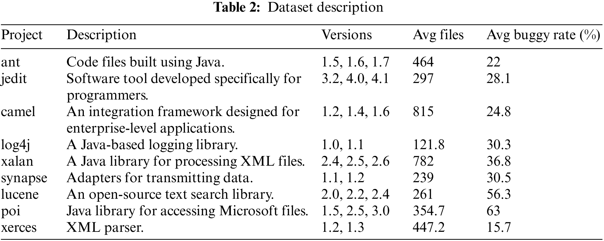
The experiments are validated in this study by utilizing the publicly accessible dataset obtained from the PROMISE repository. We specifically focus on selecting nine Java projects from the PROMISE dataset (https://github.com/ahmedabd39/promisedataset). The utilization of the PROMISE dataset in this research is motivated by two main factors. Firstly, the PROMISE dataset possesses a well-organized structure and encompasses comprehensive details concerning each project. These details include lines of code (LOC) and version numbers for individual projects. Such inclusivity facilitates the identification of defects across diverse behaviors, such as those occurring within a project or extending across multiple projects. Secondly, the PROMISE dataset incorporates real-world software projects, rendering it more pertinent to industry professionals and enabling a more authentic evaluation of the effectiveness of various approaches in predicting software defects. This aspect strengthens the practical relevance and validity of our assessments. Table 2 presents relevant details regarding the chosen projects, encompassing their project names, version numbers, concise descriptions, average source files, and average buggy rates.

4.1.2 Evaluation Metrics

The effectiveness evaluation of our software defect prediction model is conducted using two widely adopted metrics: F1-measure and AUC.

F1-measure evaluates the accuracy of a model by considering both recall and precision. It is determined by taking the harmonic mean of recall and precision, resulting in a fair evaluation of the model’s overall performance. The equations for recall, precision, and F1-measure are as follows:

Recall =TP(TP + FN)(3)

Precision =TP(TP + FP)(4)

F1−measure =2 * (Precision * Recall)(Precision + Recall)(5)

In these equations, where the True positive (TP) is the number of defective files predicted as defective. In contrast, the number of predicted defective files that are not defective is defined as the False positive (FP). False negative (FN) defines as the number of predicted defect-free files that are truly defective.

AUC (Area Under the Curve) is a frequently employed metric for assessing the effectiveness of binary classifiers. It quantifies the model’s overall performance by computing the area beneath the Receiver Operating Characteristic (ROC) curve. The ROC curve depicts the balance between the true positive rate (TPR) and the false positive rate (FPR). The equation for AUC is as follows:

AUC = integral(TPR, FPR)(6)

These evaluation metrics provide valuable insights into the performance of the proposed GB-CPDP model, allowing for a comprehensive assessment of its predictive capabilities.

4.1.3 Baseline Methods

To evaluate the efficacy of our GB-CPDP method, a comparative analysis is performed by evaluating its prediction performance against four state-of-the-art CPDP methods, as outlined below:

TPTL [30]: CPDP model that was built using a two-phase transfer learning approach. In the initial phase, TPTL uses the Source Project Estimator (SPE) tool to select source projects that are most similar in distribution to a target project from a group of possible source projects.

DA-KTSVMO [18]: DA-KTSVMO is a CPDP model incorporating an optimized quantum particle swarm optimization algorithm to enhance performance. DA-KTSVMO aimed to enhance prediction accuracy in CPDP tasks by effectively aligning training data distributions across diverse projects.

DBN [22]: Defect prediction model with syntactic features and source code change features generated by DBN. They evaluated the efficacy of their approach in the context of CPDP at both the file and change levels.

4.2 Results Analysis and Discussion

This section discusses the results of our experiments according to the following research questions:

RQ1: How does the effectiveness of the GB-CPDP approach compare to the state-of-the-art CPDP methods?

RQ2: How does the performance of GB-CPDP vary in response to external parameters?

For RQ1# As mentioned in Section 4.1.3, a comparative analysis is conducted by evaluating the prediction performance of the proposed GB-CPDP model against three baseline methods: TPTL, DA-KTSVMO, and DBN. The results in Table 3 compare the performance of the proposed GB-CPDP model against these three state-of-the-art methods in terms of AUC and F1-measure.

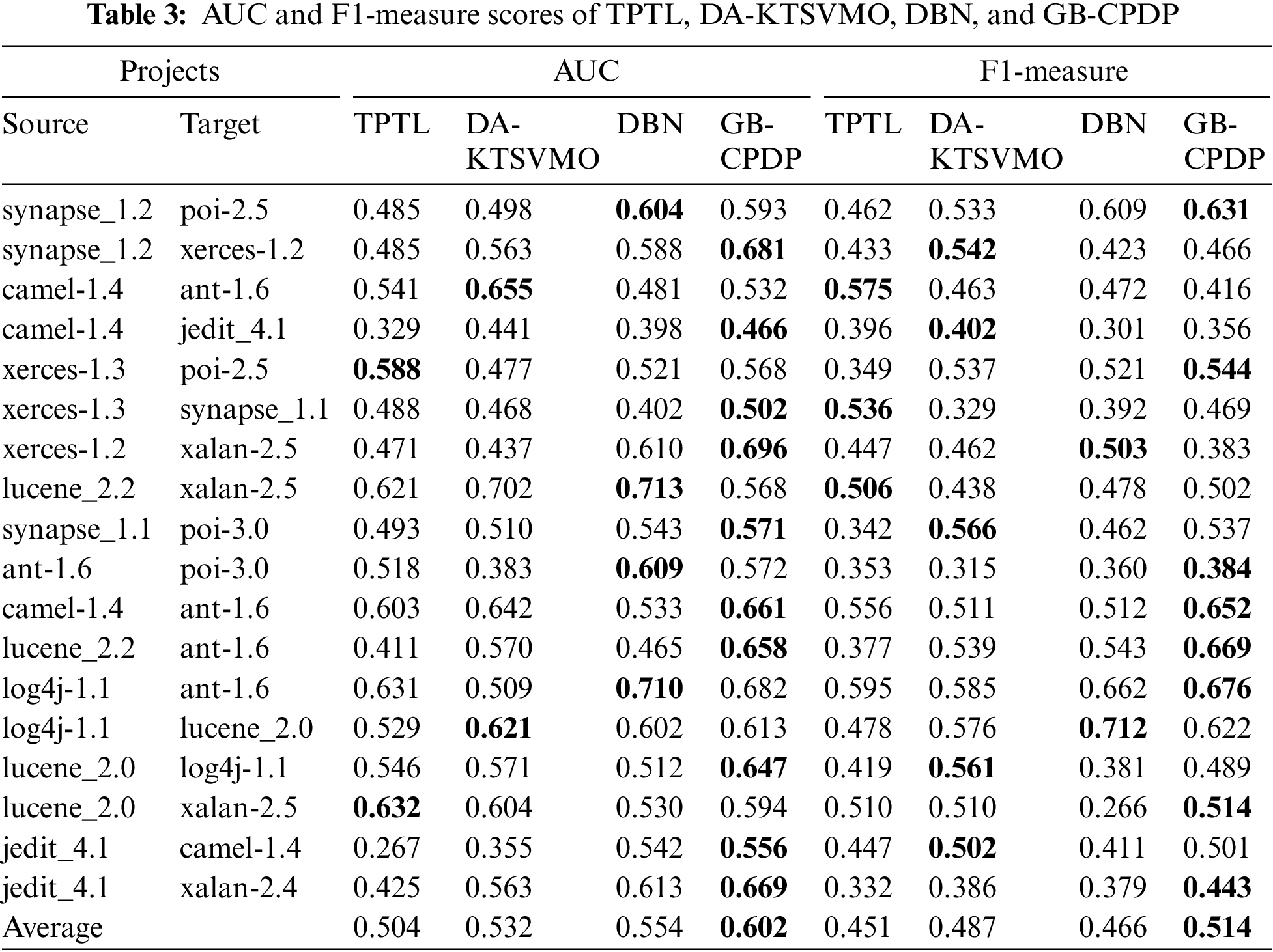
Analyzing the AUC results, the GB-CPDP model demonstrates competitive performance. It achieves an average AUC of 0.602, outperforming TPTL (0.504) and DA-KTSVMO (0.532), but being slightly outperformed by DBN (0.554). The individual dataset comparisons show that GB-CPDP consistently achieves competitive AUC scores across various source-target pairs. For example, in the synapse_1.2 to xerces-1.2 comparison, GB-CPDP achieves an AUC score of 0.681, which outperforms all the other methods. Similarly, in the log4j-1.1 to ant-1.6 comparison, GB-CPDP scores 0.682, slightly outperforming DBN’s score of 0.710. It is worth noting that there are cases where GB-CPDP’s performance is lower than that of the other methods. For instance, in the camel-1.4 to ant-1.6 comparison, GB-CPDP achieves an AUC score of 0.532, while both DA-KTSVMO and DBN achieve higher scores of 0.655 and 0.642, respectively. Table 3 also provides the F1-measure scores of the GB-CPDP model and three other state-of-the-art CPDP approaches: TPTL, DA-KTSVMO, and DBN. As shown in Table 3, the GB-CPDP model demonstrates promising results in cross-project defect prediction, outperforming the other three methods regarding the average F1-measure. The average F1-measure of GB-CPDP is 0.514, while TPTL, DA-KTSVMO, and DBN achieve average scores of 0.451, 0.487, and 0.466, respectively. This suggests that the graph-based feature learning approach, which involves extracting features from CFG and DDG using NetworkX, followed by learning with LSTM, effectively captures meaningful representations for defect prediction. The variability in performance across different project pairs is observed for all methods, indicating that the choice of source and target projects significantly impacts the predictive performance. Some project pairs show higher F1-measure scores, indicating better prediction accuracy, while others exhibit lower scores. It highlights the importance of project selection and the influence of project characteristics on the effectiveness of the CPDP methods.

In this work, Wilcoxon Signed Rank Test (WSRT) and Cliff’s delta are used to check if the performance difference between GB-CPDP and the baseline model is statistically significant. The WSRT is a statistical hypothesis test that does not rely on specific distribution assumptions. It is employed to assess if two paired samples originate from the same distribution. A p-value less than 0.05 from the test indicates a significant difference between the matched samples; otherwise, the difference is not deemed significant. To counter the influence stemming from numerous tests, the Win/Tie/Loss indicator is employed to evaluate the performance of distinct models. This approach has been utilized in previous studies to compare the performance of different methods [35,36]. The Cliff’s delta, nonparametric effect size test quantifies the practical degree of difference between two observational data sets. It serves as a complementary analysis to the WSRT. Table 4 provides the associations between Cliff’s delta (|δ|) values and their corresponding practical significance levels.

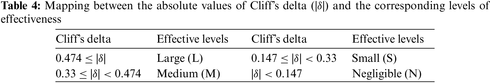
Table 5 illustrates the outcomes of Win/Tie/Loss indicators for F-measure values and AUC values. Each column presents the respective p-values of WSRT and Cliff’s delta values. The original value is shown in cases where the WSRT p-value is not less than 0.05; alternatively, if it is less than 0.05, it is replaced with “<0.05”. The corresponding practical significance level from Table 4 is employed for Cliff’s delta value. The effective level is accompanied by a “+” or “−” sign to differentiate between positive and negative Cliff’s delta values. For instance, in comparing GB-CPDP with TPTL on synapse_1.2-poi-2.56, the p-value is below 0.05, and Cliff’s delta value exceeds 0.474. Thus, the “p(δ)” of “GB-CPDP vs. TPTL” is denoted as “<0.05(+L)”. Following the Win/Tie/Loss indicator guidelines, GB-CPDP is categorized as a “Win”. By inspecting the WSRT and Cliff’s delta columns and the ‘Win/Tie/Loss’ row in Table 5, it is evident that our GB-CPDP model significantly surpasses other models in most tasks.

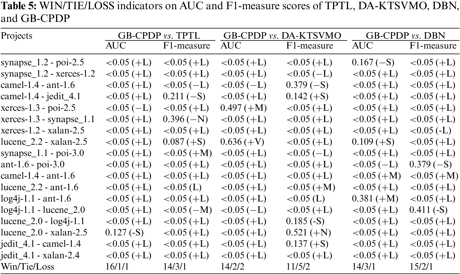
Fig. 5 presents the AUC boxplots for GB-CPDP and the three baseline methods (TPTL, DA-KTSVMO, and DBN) for all 18 experiments indicated in Table 3. Fig. 6 presents the F1-measure boxplots for GB-CPDP and the three baseline methods for all 18 experiments indicated in Table 3. For all 18 experiments, the F1-measure and AUC distribution (upper/lower and median quartiles) of each of the four approaches are presented in each boxplot. The boxplots show that GB-CPDP performs better than the four baseline approaches in F1-measure and AUC on almost all tasks. In conclusion, GB-CPDP outperforms the other baseline approaches when F1-measure and AUC are considered. These results show that semantic graph feature learning can enhance a cross-project software defect prediction.

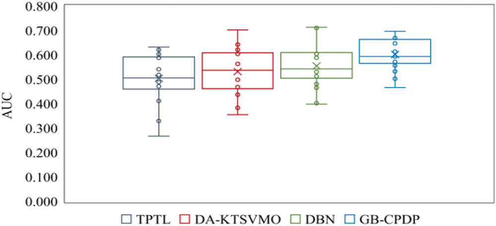
Figure 5: Comparison of AUC scores for TPTL, DA-KTSVMO, DBN, and GB-CPDP

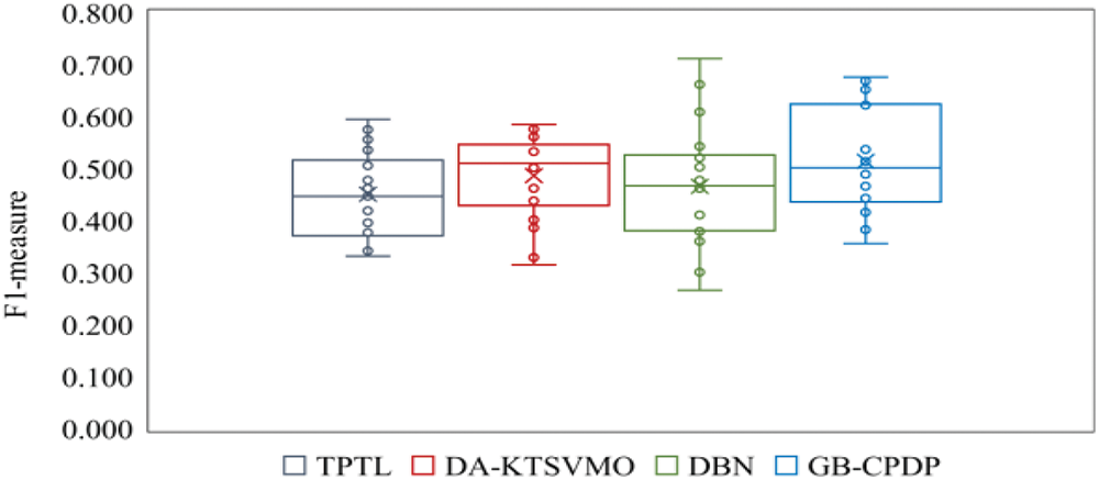
Figure 6: Comparison of F1-measure scores for TPTL, DA-KTSVMO, DBN, and GB-CPDP

In conclusion, the GB-CPDP model shows promise in CPDP, offering improved performance compared to the baseline approaches. The effective representation and prediction of defects are achieved through graph-based feature learning, which involves extracting features from CFG and DDG, along with LSTM-based learning.

For RQ2# In this section, we explore the impact of semantic graphs’ embedding dimensions as an external factor on the GB-CPDP model’s effectiveness. To determine the influence of semantic graphs’ embedding dimensions on the prediction performance of GB-CPDP, the Node2vec model is retrained using various dimension parameters: 20d, 40d, 60d, 80d, and 100d. Subsequently, the semantic features are regenerated using the corresponding Node2vec model. The F1-measure values for these 18 tasks with the five different dimensions are listed in Fig. 7.

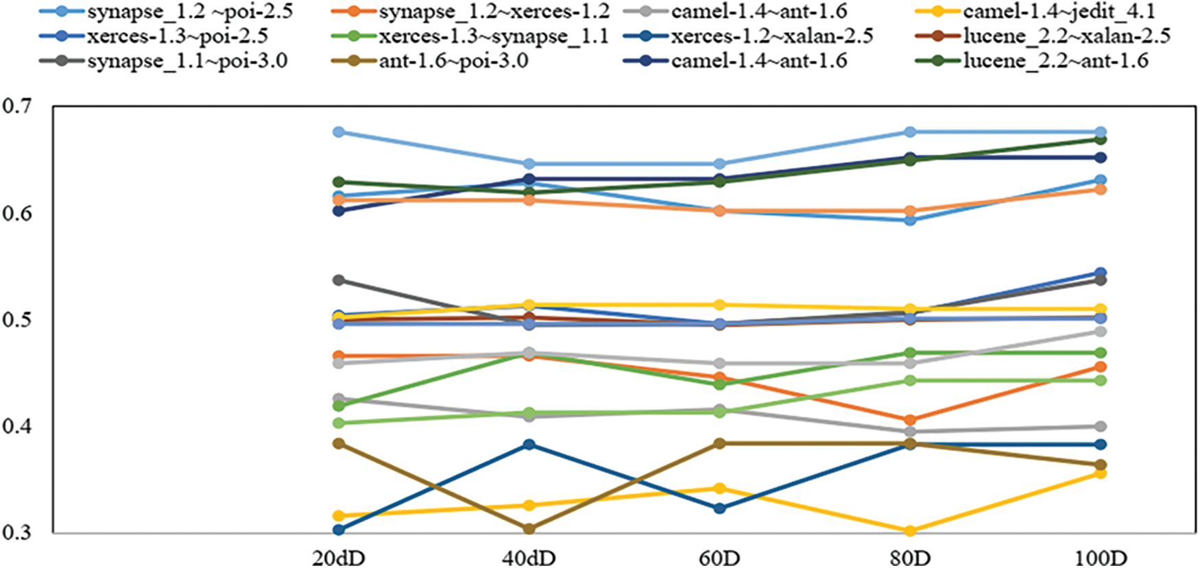
Figure 7: F1-measure of GB-CPDP under different semantic graphs’ embedding dimensions

As shown in Fig. 7, the choice of embedding dimensions significantly influences the prediction performance of the GB-CPDP model. Certain tasks exhibited higher F1-measure values with specific dimension parameters, while others displayed varied performance across the dimensions. For instance, when considering the task “synapse_1.2 poi-2.5”, the F1-measure values consistently increased from 0.602 for 20d to 0.631 for 100d. Similarly, for the task “synapse_1.1poi-3.0”, the F1-measure values improved as the dimensions increased, with the highest value recorded for 100d. On the other hand, some tasks demonstrated fluctuating F1-measure values across different dimensions. For example, the task “camel-1.4~ant-1.6” achieved the highest F1-measure value of 0.652 at 80d and 100d, while the F1-measure values were slightly lower at 60d and 40d.

These findings highlight the importance of carefully selecting the embedding dimensions for semantic graphs when using defect prediction models. It is crucial to consider the specific task and assess the performance across various dimension parameters to achieve optimal prediction accuracy.

5  Threats to Validity

5.1 Datasets Selection

A subset of nine open-source Java projects sourced from the PROMISE dataset is tested to validate our experiments. However, it should be noted that these selected projects may not represent the entirety of software projects. Furthermore, our evaluation just focused on Java projects, and therefore, the applicability of our model to other programming languages cannot be assured. As a result, our proposed method may produce varying outcomes for projects not included in the nine selected projects or those developed using different programming languages, such as Python or C.

5.2 Implementation of Baselines

Our prediction model is evaluated for comparative analysis against three state-of-the-art methods: TPTL, DA-KTSVMO, and DBN. Since these methods’ original versions were unavailable, we implemented them ourselves. While we followed the instructions provided in their respective works, it is possible that certain implementation details from the original versions may be absent in our new implementations. We used the data used in the original works to test our new implementations. We are confident that our new implementation faithfully represents the performance of these methods.

6  Conclusion

This study proposed a novel approach called GB-CPDP for cross-project software defect prediction. Our approach employed NetworkX to extract features from CFGs and DDGs. By leveraging Node2Vec, the CFGs, and DDGs have been transformed into numerical vectors, serving as graph features. LSTM was then used to learn a predictive model based on these acquired features. We conducted extensive experiments using nine Java projects from the PROMISE dataset and compared the performance of GB-CPDP with three state-of-the-art CPDP methods. Our results demonstrated that GB-CPDP outperforms the existing methods in terms of F1-measure and AUC, with improvements ranging from 2.7 to 6.3 and from 4.8 to 9.8, respectively, showcasing its efficacy in defect prediction. Despite the proposed GB-CPDP model is promising for cross-project software defect prediction, the proposed approach has limitations regarding its focus on Java projects and utilizing only CFG and DDG as graph features. While Java is a widely used programming language, the generalizability of the approach to other programming languages and domains may be limited. Additionally, relying solely on CFG and DDG may not capture all relevant contextual information for defect prediction. Other types of dependency graphs, such as Value Dependency Graphs (VDG), could provide additional insights and improve the model’s accuracy.

There are several avenues for future research and improvements. For example, extending the evaluation to a broader range of software projects, encompassing different programming languages such as C++ and Python and domains such as Mobile Apps, would provide a more comprehensive understanding of GB-CPDP’s performance. Exploring and incorporating other graph-based features beyond the CFG and DDG could further enhance the predictive capabilities of GB-CPDP. For example, data flow or module dependency graphs may capture additional contextual information relevant to defect prediction.

Acknowledgement: We are indebted to the Institute of Information & Communications Technology Planning & Evaluation (IITP) for supporting this work and all members who contributed to this work.

Funding Statement: This work was supported by Institute of Information & Communications Technology Planning & Evaluation (IITP) grant funded by the Korea government (MSIT) (No. RS-2022-00155885).

Author Contributions: Conceptualization, Ahmed Abdu; Methodology, Ahmed Abdu, Hakim A. Abdo and Zhengjun Zhai; Software, Ahmed Abdu, Redhwan Algabri and Hakim A. Abdo; Validation, Ahmed Abdu, Redhwan Algabri, Sungon Lee and Zhengjun Zhai; Formal analysis, Redhwan Algabri; Investigation, Ahmed Abdu, Hakim A. Abdo and Zhengjun Zhai; Resources, Zhengjun Zhai; Data Curation, Ahmed Abdu, Redhwan Algabri and Zhengjun Zhai; Writing—original draft, Ahmed Abdu.; Writing—review & editing, Redhwan Algabri and Sungon Lee; Visualization, Ahmed Abdu, Hakim A. Abdo and Zhengjun Zhai; Supervision, Zhengjun Zhai; Funding acquisition, Zhengjun Zhai and Sungon Lee; Project administration, Zhengjun Zhai and Sungon Lee. All authors have read and agreed to the published version of the manuscript.

Availability of Data and Materials: The data used in this paper can be requested from the corresponding author upon request.

Conflicts of Interest: The authors declare that they have no conflict of interest to report regarding the present study.

References

1. C. Ni, X. Chen, F. Wu, Y. Shen and Q. Gu, “An empirical study on pareto based multi-objective feature selection for software defect prediction,” Journal of Systems and Software, vol. 152, no. 1, pp. 215–238, 2019. [Google Scholar]

2. Z. Wan, X. Xia, A. E. Hassan, D. Lo, J. Yin et al., “Perceptions, expectations, and challenges in defect prediction,” IEEE Transactions on Software Engineering, vol. 46, no. 11, pp. 1241–1266, 2018. [Google Scholar]

3. E. Rashid and M. D. Ansari, “Fixing the bugs in software projects from software repositories for improvisation of quality,” Recent Advances in Electrical & Electronic Engineering, vol. 13, no. 2, pp. 184–192, 2020. [Google Scholar]

4. U. Sharma and R. Sadam, “How far does the predictive decision impact the software project? The cost, service time, and failure analysis from a cross-project defect prediction model,” Journal of Systems and Software, vol. 195, no. 13, pp. 111522, 2023. [Google Scholar]

5. M. D. Ansari and S. P. Ghrera, “Intuitionistic fuzzy local binary pattern for features extraction,” International Journal of Information and Communication Technology, vol. 13, no. 1, pp. 83–98, 2018. [Google Scholar]

6. E. Rashid, M. Prakash, M. D. Ansari and V. K. Gunjan, “Formalizing open source software quality assurance model by identifying common features from open source software projects,” in ICCCE 2020: Proc. of the 3rd Int. Conf. on Communications and Cyber Physical Engineering, Hyderabad, Telangana, India, Springer, pp. 1375–1384, 2021. [Google Scholar]

7. F. Wu, X. Y. Jing, Y. Sun, J. Sun, L. Huang et al., “Cross-project and within-project semisupervised software defect prediction: A unified approach,” IEEE Transactions on Reliability, vol. 67, no. 2, pp. 581–597, 2018. [Google Scholar]

8. H. Tong, B. Liu and S. Wang, “Software defect prediction using stacked denoising autoencoders and two-stage ensemble learning,” Information and Software Technology, vol. 96, no. 1, pp. 94–111, 2018. [Google Scholar]

9. J. Chen, K. Hu, Y. Yang, Y. Liu and Q. Xuan, “Collective transfer learning for defect prediction,” Neurocomputing, vol. 416, pp. 103–116, 2020. [Google Scholar]

10. K. Shi, Y. Lu, J. Chang and Z. Wei, “PathPair2Vec: An AST path pair-based code representation method for defect prediction,” Journal of Computer Languages, vol. 59, pp. 100979, 2020. [Google Scholar]

11. Y. Zhao, Y. Zhu, Q. Yu and X. Chen, “Cross-project defect prediction considering multiple data distribution simultaneously,” Symmetry, vol. 14, no. 2, pp. 401, 2022. [Google Scholar]

12. W. Jiang, S. Qiu, T. Liang and F. Zhang, “Cross-project clone consistent-defect prediction via transfer-learning method,” Information Sciences, vol. 635, no. 1, pp. 138–150, 2023. [Google Scholar]

13. T. Zimmermann, N. Nagappan, H. Gall, E. Giger and B. Murphy, “Cross-project defect prediction: A large scale experiment on data vs. domain vs. process,” in Proc. of the 7th Joint Meeting of the European Software Engineering Conf. and the ACM SIGSOFT Symp. on the Foundations of Software Engineering, Amsterdam, Netherlands, pp. 91–100, 2009. [Google Scholar]

14. C. Ni, W. S. Liu, X. Chen, Q. Gu, D. X. Chen et al., “A cluster based feature selection method for cross-project software defect prediction,” Journal of Computer Science and Technology, vol. 32, no. 6, pp. 1090–1107, 2017. [Google Scholar]

15. Z. Xu, P. Yuan, T. Zhang, Y. Tang, S. Li et al., “HDA: Cross-project defect prediction via heterogeneous domain adaptation with dictionary learning,” IEEE Access, vol. 6, pp. 57597–57613, 2018. [Google Scholar]

16. S. Qiu, L. Lu and S. Jiang, “Multiple-components weights model for cross-project software defect prediction,” IET Software, vol. 12, no. 4, pp. 345–355, 2018. [Google Scholar]

17. K. Zhu, N. Zhang, S. Ying and X. Wang, “Within-project and cross-project software defect prediction based on improved transfer naive bayes algorithm,” Computers, Materials & Continua, vol. 63, no. 2, pp. 891–910, 2020. [Google Scholar]

18. C. Jin, “Cross-project software defect prediction based on domain adaptation learning and optimization,” Expert Systems with Applications, vol. 171, no. 1, pp. 114637, 2021. [Google Scholar]

19. Y. Sun, Y. Sun, J. Qi, F. Wu, Y. Jing et al., “Unsupervised domain adaptation based on discriminative subspace learning for cross-project defect prediction,” Computers, Materials & Continua, vol. 68, no. 3, pp. 3373–3389, 2021. [Google Scholar]

20. J. Bai, J. Jia and L. F. Capretz, “A three-stage transfer learning framework for multi-source cross-project software defect prediction,” Information and Software Technology, vol. 150, pp. 106985, 2022. [Google Scholar]

21. Z. Sun, J. Li, H. Sun and L. He, “CFPS: Collaborative filtering based source projects selection for cross-project defect prediction,” Applied Soft Computing, vol. 99, no. 6, pp. 106940, 2021. [Google Scholar]

22. S. Wang, T. Liu, J. Nam and L. Tan, “Deep semantic feature learning for software defect prediction,” IEEE Transactions on Software Engineering, vol. 46, no. 12, pp. 1267–1293, 2018. [Google Scholar]

23. D. Chen, X. Chen, H. Li, J. Xie and Y. Mu, “DeepCPDP: Deep learning based cross-project defect prediction,” IEEE Access, vol. 7, pp. 184832–184848, 2019. [Google Scholar]

24. C. Ni, X. Xia, D. Lo, X. Chen and Q. Gu, “Revisiting supervised and unsupervised methods for effort-aware cross-project defect prediction,” IEEE Transactions on Software Engineering, vol. 48, no. 3, pp. 786–802, 2020. [Google Scholar]

25. F. Zhang, A. Mockus, I. Keivanloo and Y. Zou, “Towards building a universal defect prediction model with rank transformed predictors,” Empirical Software Engineering, vol. 21, no. 5, pp. 2107–2145, 2016. [Google Scholar]

26. A. Abdu, Z. Zhai, R. Algabri, H. A. Abdo, K. Hamad et al., “Deep learning-based software defect prediction via semantic key features of source code—systematic survey,” Mathematics, vol. 10, no. 17, pp. 3120, 2022. [Google Scholar]

27. B. Turhan, T. Menzies, A. B. Bener and J. di Stefano, “On the relative value of cross-company and within-company data for defect prediction,” Empirical Software Engineering, vol. 14, no. 5, pp. 540–578, 2009. [Google Scholar]

28. N. Limsettho, K. E. Bennin, J. W. Keung, H. Hata and K. Matsumoto, “Cross project defect prediction using class distribution estimation and oversampling,” Information and Software Technology, vol. 100, pp. 87–102, 2018. [Google Scholar]

29. D. Ryu, O. Choi and J. Baik, “Value-cognitive boosting with a support vector machine for cross-project defect prediction,” Empirical Software Engineering, vol. 21, pp. 43–71, 2016. [Google Scholar]

30. C. Liu, D. Yang, X. Xia, M. Yan and X. Zhang, “A two-phase transfer learning model for cross-project defect prediction,” Information and Software Technology, vol. 107, pp. 125–136, 2019. [Google Scholar]

31. A. K. Goel, R. Chakraborty, M. Agarwal, M. D. Ansari, S. K. Gupta et al., “Profit or loss: A long short term memory based model for the prediction of share price of DLF group in India,” in 2019 IEEE 9th Int. Conf. on Advanced Computing (IACC), Tamilnadu, India, IEEE, pp. 120–124, 2019. [Google Scholar]

32. H. Liang, Y. Yu, L. Jiang and Z. Xie, “SEML: A semantic LSTM model for software defect prediction,” IEEE Access, vol. 7, pp. 83812–83824, 2019. [Google Scholar]

33. A. Majd, M. Vahidi-Asl, A. Khalilian, P. Poorsarvi-Tehrani and H. Haghighi, “SLDeep: Statement-level software defect prediction using deep-learning model on static code features,” Expert Systems with Applications, vol. 147, pp. 113156, 2020. [Google Scholar]

34. J. Deng, L. Lu and S. Qiu, “Software defect prediction via LSTM,” IET Software, vol. 14, no. 4, pp. 443–450, 2020. [Google Scholar]

35. H. Wang, W. Zhuang and X. Zhang, “Software defect prediction based on gated hierarchical LSTMs,” IEEE Transactions on Reliability, vol. 70, no. 2, pp. 711–727, 2021. [Google Scholar]

36. G. Fan, X. Diao, H. Yu, K. Yang and L. Chen, “Deep semantic feature learning with embedded static metrics for software defect prediction,” in 2019 26th Asia-Pacific Software Engineering Conf. (APSEC), Putrajaya, Malaysia, IEEE, pp. 244–251, 2019. [Google Scholar]