
 Submit a Paper
 Propose a Special lssue
 Open Access
ARTICLE
EMU-Net: Automatic Brain Tumor Segmentation and Classification Using Efficient Modified U-Net
1 Department of Artificial Intelligence, Faculty of Artificial Intelligence, Egyptian Russian University, Badr City, 11829, Egypt
2 Computer Science Department, Shaqra University, Shaqra City, 11961, Saudi Arabia
* Corresponding Author: Mohammed Aly. Email:
Computers, Materials & Continua 2023, 77(1), 557-582. https://doi.org/10.32604/cmc.2023.042493
Received 01 June 2023; Accepted 11 August 2023; Issue published 31 October 2023
 View Full Text
 Download PDF
Abstract
Tumor segmentation is a valuable tool for gaining insights into tumors and improving treatment outcomes. Manual segmentation is crucial but time-consuming. Deep learning methods have emerged as key players in automating brain tumor segmentation. In this paper, we propose an efficient modified U-Net architecture, called EMU-Net, which is applied to the BraTS 2020 dataset. Our approach is organized into two distinct phases: classification and segmentation. In this study, our proposed approach encompasses the utilization of the gray-level co-occurrence matrix (GLCM) as the feature extraction algorithm, convolutional neural networks (CNNs) as the classification algorithm, and the chi-square method for feature selection. Through simulation results, the chi-square method for feature selection successfully identifies and selects four GLCM features. By utilizing the modified U-Net architecture, we achieve precise segmentation of tumor images into three distinct regions: the whole tumor (WT), tumor core (TC), and enhanced tumor (ET). The proposed method consists of two important elements: an encoder component responsible for down-sampling and a decoder component responsible for up-sampling. These components are based on a modified U-Net architecture and are connected by a bridge section. Our proposed CNN architecture achieves superior classification accuracy compared to existing methods, reaching up to 99.65%. Additionally, our suggested technique yields impressive Dice scores of 0.8927, 0.9405, and 0.8487 for the tumor core, whole tumor, and enhanced tumor, respectively. Ultimately, the method presented demonstrates a higher level of trustworthiness and accuracy compared to existing methods. The promising accuracy of the EMU-Net study encourages further testing and evaluation in terms of extrapolation and generalization.Keywords
Numerous deadly diseases impact the modern world, and one of them is brain tumors. These tumors can develop in various locations within the human brain and come in different sizes and shapes. Brain tumors can be categorized as either benign (non-cancerous) or malignant (cancerous). There are four grades (I to IV) used to classify brain tumors [1]. Grades I and II indicate benign tumors, while grades III and IV refer to malignant ones. Tumors can originate within the brain (primary type) or start elsewhere in the body and spread to the brain (secondary type). The most common type of brain tumor is glioma, which primarily affects adults and children. Gliomas are formed by abnormal glial cells in the brain and are further classified into high-grade glioma (HGG) and low-grade glioma (LGG). Notably, HGG has a median survival time (MST) of only 15 months [2]. Accurate detection and an effective treatment plan are vital in increasing patient survival rates. In the field of medicine, imaging techniques play a crucial role in analyzing the human body. Among the various available methods, magnetic resonance imaging (MRI) is highly beneficial in swiftly diagnosing brain tumors and generating multimodal images [3]. By utilizing radio waves and magnetic fields, MRI produces detailed pictures of the human body. MR images are created using two distinct signals: time to echo (TE) and repetition time (TR).
The presence of multimodal images in MRI makes manual segmentation of brain tumors challenging and time-consuming. Therefore, the development of a fully automated segmentation technique is necessary to address this issue. Numerous automated segmentation methods have been developed; however, achieving accuracy remains a significant challenge due to the absence of clear boundaries between tumor and normal brain cells [4]. MRI generates multimodal images such as T1-weighted (T1W), T2-weighted (T2W), T1 with contrast (T1C), and Fluid Attenuated Inversion Recovery (FLAIR) images. Each MRI modality represents a specific part of the brain tissue, with FLAIR images representing the entire tumor area. Refer to Fig. 1 for an illustration of the different types of MRI multimodal images.

Figure 1: MRI multimodal. (A) T1W, (B) T2W, (C) FLAIR and (D) T1C
The primary objective of tumor segmentation is to divide the pixels in an image into regions that exhibit similar characteristics [5]. When segmenting brain tumors, the main goal is to identify specific sections of the tumor, namely the tumor core (TC), enhancing tumor (ET), and whole tumor (WT). There are two primary approaches for brain tumor segmentation: discriminative and generative. The discriminative method relies on prior knowledge and fine-grained features in the images, learning from trained examples. On the other hand, the generative method utilizes previous knowledge about normal tissues and tumors [6]. In Fig. 2, a visual representation of the substructure of a brain tumor is depicted.
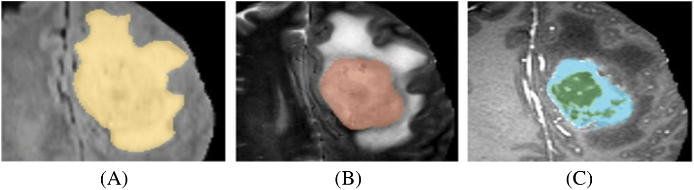
Figure 2: Brain tumor substructures. (A) WT, (B) TC, (C) ET
In recent times, there has been an increased utilization of deep-learning methods in both the classification [7] and segmentation [8] of brain tumors. These methods extract semantic features from the images and assign class labels accordingly. The field of computer vision is employed to extract new information from digital images. Among the concepts in artificial neural networks, the convolutional neural network (CNN) is widely employed for segmentation and classification purposes. The neural network comprises three layers: input, hidden, and output. The input layer receives data that is then propagated through the rest of the network. The hidden layer plays a vital role in ensuring the network’s efficient performance, possessing an automatic feature extraction function and facilitating data transformation. The output layer stores the final results. For biomedical image segmentation, the U-Net is a popular CNN-based architecture. Its name derives from its U-shaped design and its core, which is a fully convolutional network. The U-Net is specifically designed to achieve accurate segmentation results even with limited training images [9]. The architecture of U-Net consists of two components: the encoder and the decoder. These components form the first and second parts of the network. The encoder employs down-sampling techniques, while the decoder utilizes up-sampling techniques.
In order to address the limitations observed in other brain tumor segmentation models like U-Net, such as inadequate edge detail segmentation, ineffective feature information reuse, subpar extraction of location information, and the inefficacy of commonly used binary cross-entropy and Dice loss functions, we propose a novel solution. Our proposed approach involves a serial encoding-decoding structure that enhances segmentation performance through the addition and concatenation of each module in two modified U-Net serial networks.
This research paper focuses on the utilization of the Brain Tumor Segmentation (BraTS) 2020 multimodal dataset. Two types of brain tumor classification are performed: (A) feature extraction using the Gray Level Co-occurrence Matrix (GLCM) and (B) a proposed Convolutional Neural Network (CNN). The best classification result is selected from these two methods. The brain tumor segmentation is accomplished using an efficient modified U-Net (EMU-Net) segmentation architecture. In this approach, we enhance the low-level features by adding additional residual blocks to all encoder path layers, transforming them into high-level features. The proposed method comprises two crucial components: the encoder component (down-sampling) and the decoder component (up-sampling), with a bridge section connecting the two modified U-Net architecture. This modification leads to improved segmentation results.
The remaining sections of the document are as follows: Section 2 describes the research on classifying and segmenting brain tumors. Section 3 lists the materials, metrics, and tools utilized in this research article. Section 4 presents our new suggested technique for tumor classification and segmentation. Section 5 notes the outcomes of the suggested method, including comparisons with state-of-the-art methods. Finally, Section 6 concludes the research study.
In the medical field, brain tumor segmentation is a crucial process that helps doctors accurately identify different parts of the tumor. Various automatic brain tumor segmentation techniques have been developed, facilitating the segmentation process for doctors. Pereira et al. [10] used a deep Convolutional Neural Network (CNN) architecture consisting of three kernel layers for brain tumor classification. They utilized the BraTS 2013 and 2015 datasets and incorporated three stages: pre-processing, CNN-based classification, and post-processing. In their study, Chen et al. [11] utilized the MU-Net, a novel convolutional network with multiple paths for upsampling, to preserve a greater amount of high-level information. The MU-Net architecture is primarily composed of three essential components: a contracting path, skip connections, and multiple expansive paths. The performance of the proposed MU-Net architecture has been assessed using three distinct medical imaging datasets.
Deep CNN is widely used in brain tumor segmentation due to its advantages of low training requirements, data augmentation, and faster processing time. Hussain et al. [12] developed a fully automatic segmentation method using deep CNN on the BraTS 2013 dataset. They employed two types of image patches, 37 × 37 and 19 × 19, and incorporated max-pooling, max-out, and dropout layers to enhance training and testing speed. Iqbal et al. [13] implemented deep CNN for tumor segmentation, creating three networks: skipNet, Interpolated Network (Internet), and SE-Net, with an encoder and decoder architecture on the BraTS 2015 dataset. Their method involved pre-processing, training, and obtaining results based on a test dataset.
Wang et al. [14] developed a fully automated brain tumor segmentation technique using an underlying network architecture. They utilized three networks: 3D UNet, cascaded network, and WNet, with training and testing involving 3D rotation and flipping of the images. They employed metrics such as Hausdorff distance and dice score for tumor comparison with ground truth images. Thaha et al. [15] introduced a new technique called Enhanced Convolutional Neural Networks for Segmentation (ECNN), incorporating the BAT algorithm for the loss function. Their approach focused on optimization-based MRI segmentation and employed small-size kernels to achieve a deep architecture.
Thillaikkarasi et al. [16] combined CNN and Multiclass Support Vector Machine (M-SVM) for tumor segmentation. They used pre-processing techniques such as Contrast Limited Adaptive Histogram Equalization (CLAHE) and Laplacian of Gaussian Filtering (LOG), along with the Statistical Gray Level Difference Method (SGLDM) for feature extraction. Zhou et al. [17] employed a 3D-Method Atrous-Convolution Feature Pyramid Network (AFPNet) to locate brain tumors, addressing spatial information loss and weak points in multi-scale tumor processing. Their method incorporated fully connected conditional random fields for post-processing.
Zeineldin et al. [18] developed a modified U-Net architecture for tumor segmentation based on the BraTS 2019 dataset. Their approach involved feature extraction in the encoder part and image up-sampling in the decoder part, focusing only on FLAIR-type MR images. Kalaiselvi et al. [19] created six distinct CNN models for tumor classification, with the sixth model achieving superior results. They incorporated five layers, batch normalization, and dropout techniques, although their method required more computational time.
Chen et al. [20] implemented the Deep Convolution Symmetric Neural Network (DCSNN) for brain tumor segmentation, incorporating symmetric masks in multiple layers and using a left-right similarity metric for whole tumor segmentation. Vijh et al. [21] devised a hybrid adaptive Particle Swarm Optimization (PSO) and OTSU technique for brain tumor segmentation, utilizing both non-tumor and tumor images from the Internet Brain Segmentation Repository (IBSR) dataset. They employed skull stripping for pre-processing and achieved 98% accuracy using CNN.
In the study conducted by Preethi et al. [22], wavelet texture features and deep neural networks (DNNs) were utilized for brain tumor classification. The feature matrix was generated by combining wavelet texture features (GLCM) and wavelet GLCM. Subsequently, the brain images were categorized using the DNN based on the selected features. The results indicated that the classifier achieved a total sensitivity, specificity, and accuracy of 86%, 90%, and 88%, respectively.
In the study conducted by Widhiarso et al. [23], the researchers employed the Gray Level Co-occurrence Matrix (GLCM) to analyze brain tumor data. The primary objective of this research was to process the extracted information from the GLCM and apply it to a Convolutional Neural Network (CNN) to achieve accurate measurements. For the training and retraining of the CNN, four different combinations of tumor data (Meningioma, Glioma, and Pituitary Tumor) from TI1 were utilized. The training process involved 14 combinations of GLCM features using the Mg-Gl, Mg-Pt, Gl-Pt, and Mg-Gl-Pt datasets. The results obtained from this method on the respective datasets demonstrated an overall accuracy of 50% for Mg-Gl, 76% for Mg-Pt, 82% for Gl-Pt, and 54% for Mg-Gl-Pt.
Munajat et al. [24] conducted a study where they employed the Gray Level Co-occurrence Matrix (GLCM) to detect brain tumors. The GLCM generated values like Contrast, Homogeneity, Energy, and Correlation, which were subsequently utilized in a classification approach using the Backpropagation Neural Network algorithm. The results demonstrated that the highest accuracy was achieved when utilizing a GLCM parameter with a distance (
To address the remaining challenges faced by the U-Net network, several approaches have been proposed. Alom introduced a recursive neural network and a recursive residual convolution neural network based on the U-Net model [25]. Zhang et al. extended the U-Net path with residual connections and presented a depth residual U-Net for image segmentation [26]. Milletari et al. proposed a 3D U-Net model that expanded the original structure using a 3D convolution kernel and incorporated residual units for further modification [27]. Salehi et al. employed an auto-context algorithm to enhance U-Net and improve segmentation effectiveness [28]. Zhou et al. replaced the original connection method with a nesting approach [29]. Chen et al. introduced a stacked U-Net with a bridging structure to tackle the increasing training difficulty as the network’s layer count grows [30]. However, these segmentation models are limited to image segmentation and do not encompass tumor grading. In order to fulfill this clinical requirement, Naser et al. employed a trained segmentation model and MRI images to generate masks, which were subsequently classified using a densely connected neural network classifier [31].
3 Materials, Metrics, and Tool
The BraTS initiative aims to foster collaboration within the research community and encourage the development of innovative solutions to various challenges. As part of this initiative, benchmark datasets are made available, specifically designed for the segmentation task. The organizers provide a diverse range of independent datasets for training, validation, and testing purposes in BraTS competitions. In this manuscript, we utilized the BraTS2020 dataset, which consists exclusively of glioma-type tumor images [32]. The dataset comprises a total of 369 patient images, with 259 High-Grade Glioma (HGG) and 110 Low-Grade Glioma (LGG) cases. Each patient’s MRI multimodal data includes T1W, T2W, T1C, and FLAIR, along with corresponding ground truth MR images. The MRI multimodal data is stored in separate folders, with each folder containing 155 image slices. It is important to note that all BraTS images are exclusively available in the neuroimaging informatics technology initiative (NIfti) file format [33].
Several evaluation criteria have been devised to assess the performance of classification and segmentation results. This article utilizes three classification metrics: sensitivity, specificity, and accuracy. Additionally, for brain tumor segmentation, the Dice Coefficient is employed along with the aforementioned metrics. The Dice metric is commonly used in the segmentation of MR images of brain tumors and serves as a benchmark for result comparison in many studies. The Eqs. (1) to (4) below represent the metrics utilized in this evaluation: Eq. (1): Sensitivity, Eq. (2): Specificity, Eq. (3): Accuracy, and Eq. (4): Dice Coefficient.
True positive (TP) refers to the number of pixels that are correctly identified as a tumor. False positive (FP) represents the number of pixels that are actually normal but are incorrectly identified as a tumor. True negative (TN) indicates the number of pixels correctly identified as normal tissues. False negative (FN) denotes the number of pixels that are a tumor but are incorrectly identified as normal tissues.
This paper utilized MATLAB R2021a (academic version) for the MR image classification and tumor image segmentation process. MATLAB, also known as Matrix Laboratory, is particularly used for image processing. The method employed an Intel® i5-2430M CPU @ 2.40 GHz and 8 GB RAM as hardware specifications. Matlab utilized machine learning methods to classify the images and also included built-in medical image segmentation algorithms [34].
This paper comprises two main phases: brain tumor classification and segmentation. The MRI multimodal images from the dataset were utilized for this purpose. The classification process involved two approaches: Method (A) utilizing the GLCM method and Method (B) employing CNN. Both classification methods used the same labels: tumor (1) and normal (0). Subsequently, the results of Method A and Method B were compared, and the best result was selected for further segmentation. The segmentation process involved dividing the tumor images into three parts: tumor core, enhanced tumor, and whole tumor, using our modified U-Net architecture called EMU-Net. The complete workflow diagram illustrating the developed methodology is presented in Fig. 3.
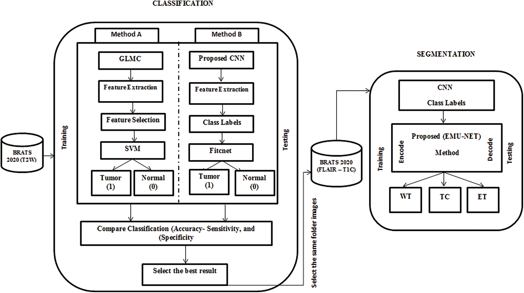
Figure 3: Proposed EMU-Net method workflow diagram
Classification plays a crucial role in the medical field [35–37], and this manuscript specifically focuses on T2W images from the dataset. The MR images of the BraTS type do not require any pre-processing steps such as head stripping or noise removal. Each grayscale image has dimensions of 240 × 240 × 1 pixels. All T2W images from the 369 patients were used in this study, resulting in a dataset containing a total of 57,195 images (369 × 155). For classification, a combination of High-Grade Glioma (HGG) and Low-Grade Glioma (LGG) images was utilized, with 45,756 (80%) images used for training and 11,439 (20%) images used for testing. The method extracts relevant features and selects the best ones for classification. The manuscript compares the results obtained from the Method A and Method B approaches and subsequently selects the superior one. Fig. 4 shows CNN is combination of Feedforward and fully-connected layer.
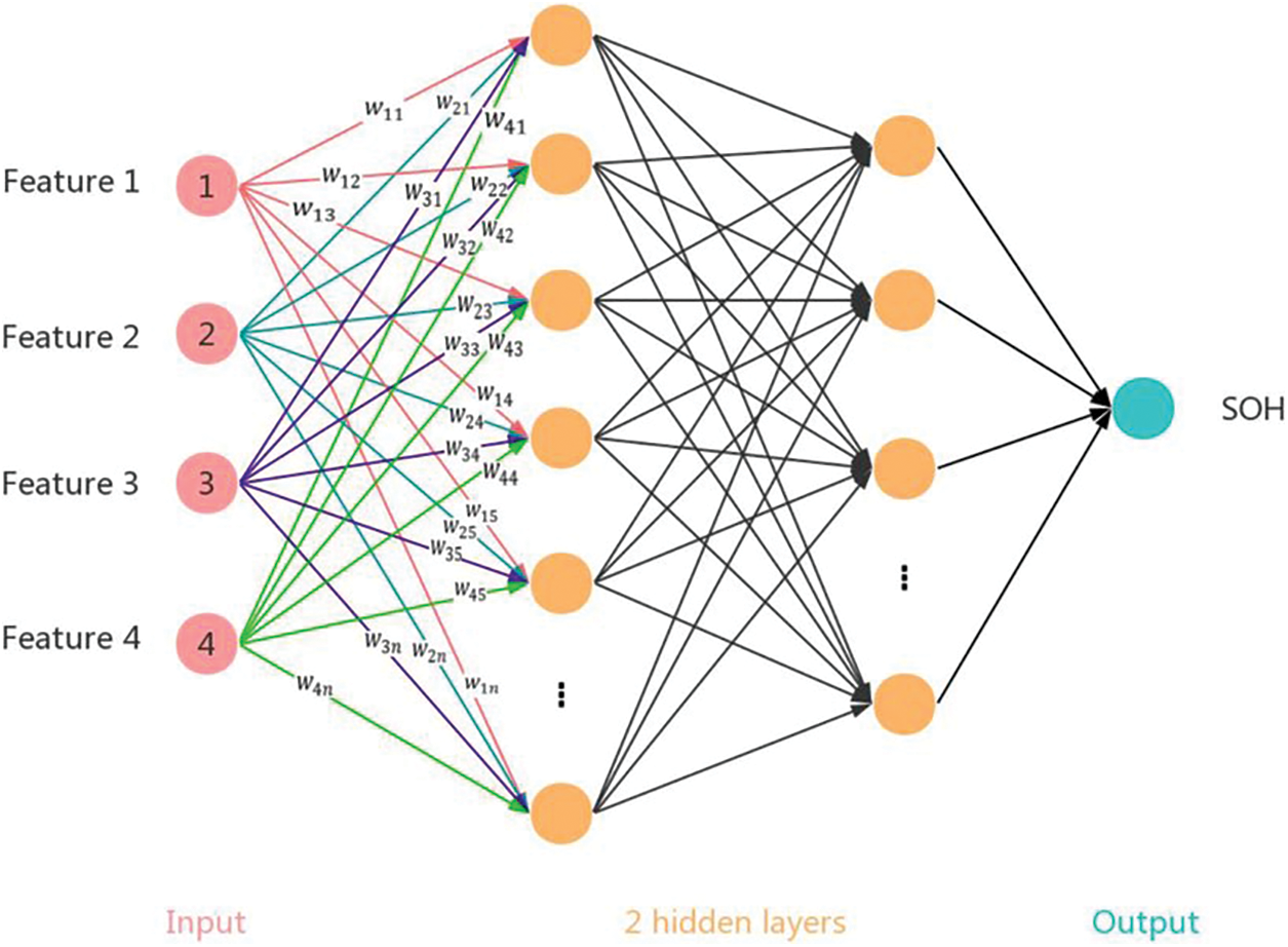
Figure 4: Illustrates a fully connected 3-layer feedforward neural network and a convolutional neural network (CNN) with a convolutional layer as the first layer and a pooling layer as the second layer. In the CNN, the filter size is 2 × 2 with a stride of (1,1), and the pooling size is 1 × 3 with a stride of (1,1)
4.1.1 Method A-Classification Using the GLCM Method
In this approach, feature extraction plays a vital role as each feature provides specific information about individual pixels. The GLCM method is employed to extract nineteen features from both the training and testing images. The co-occurrence matrix captures texture and spatial features [38]. The GLCM technique encompasses projection angles at different orientations, including 0°, 45°, 90°, and 135°. For this method, the 45° projection angle is utilized. The specific reason to choose the angle of 45 degrees in GLCM is to capture diagonal texture patterns within an image. This angle allows for the detection of diagonal relationships between pixels, which can be useful for identifying diagonal texture features or structures present in the image. Fig. 5 illustrates the starting pixel of the image, denoted by a gray-colored pixel box. The different types of projection angles are depicted in Fig. 5. The extracted features, totaling nineteen, for the resulting images are presented in Table 1. Fig. 6 presents the GLCM feature extraction flowchart.
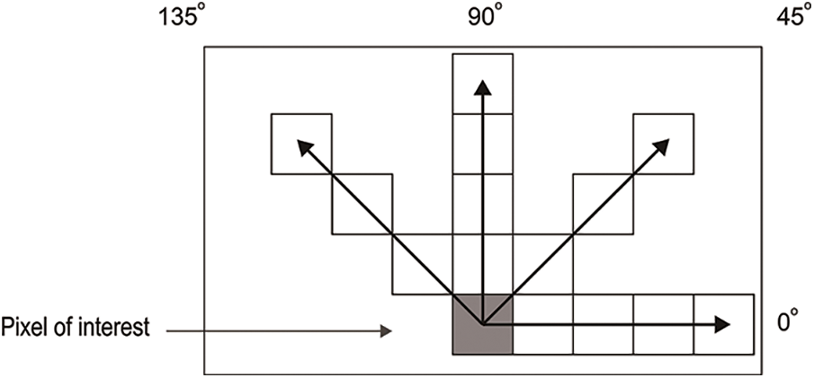
Figure 5: GLCM projection angles
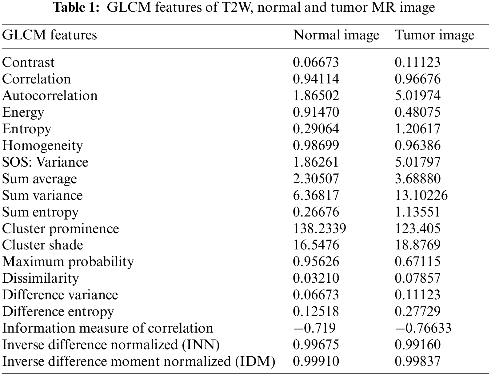
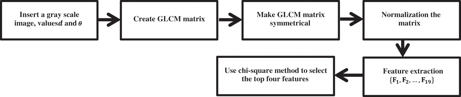
Figure 6: GLCM feature extraction flowchart
The input for this method consists of the nineteen GLCM features extracted from both normal and tumor images, along with the corresponding response variables. In this approach, two response variables are utilized: normal (0) and tumor (1). Not all GLCM feature values are employed for classification; instead, a selection process is carried out using the chi-square test method [39]. This method compares each feature with the response variable and generates a feature rank based on their relevance. The feature selection rank is visualized through a bar chart, as depicted in Fig. 7.
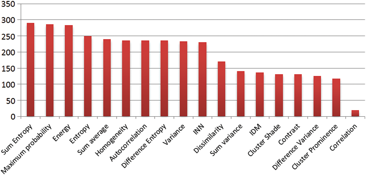
Figure 7: Feature selection rank bar chart
The goal of feature selection is to identify the most relevant features or variables that contribute the most to the predictive power of a model [40]. A chi-square test measures the independence between two categorical variables. It determines whether there is a significant association or relationship between the variables based on their observed frequencies. In the context of feature selection, the chi-square test can be used to assess the association between each individual feature and the target variable. Here is a step-by-step process of using chi-square tests for feature selection:
1. Define the problem: Determine the classification task you are working on and the target variable you want to predict.
2. Preprocess the data: Ensure that all variables are categorical or can be discretized into categories. If necessary, transform continuous variables into categorical ones through binning or other methods.
3. Calculate the chi-square statistic: For each feature, compute the chi-square statistic by comparing the observed frequencies with the expected frequencies under the assumption of independence between the feature and the target variable. This can be done using a contingency table, which cross-tabulates the feature and the target variable.
4. Determine the degrees of freedom: The degrees of freedom in the chi-square test depend on the number of categories in both the feature and the target variable. The formula is
5. Evaluate the p-value: Calculate the p-value associated with each chi-square statistic. The p-value indicates the probability of observing the association between the feature and the target variable by chance, assuming they are independent. Lower p-values suggest a stronger association.
6. Set a significance level: Choose a significance level (e.g., 0.05) to determine the threshold for statistical significance. Features with p-values below this threshold are considered statistically significant.
7. Select features: Based on the p-values, select the features that have p-values below the significance level. These features are considered to have a significant association with the target variable and can be included in your model.
The Chi-square test is well-suited for the BraTS dataset due to several reasons:
- Categorical Variables: The Chi-square test is designed to examine associations between categorical variables. In the context of BraTS, the dataset may contain categorical variables representing different tumor characteristics or regions. By using the Chi-square test, we can effectively investigate these variables.
- Independence Testing: The Chi-square test is commonly employed to determine the independence between variables. In the case of BraTS, it helps assess the independence between features (e.g., imaging features) and the target variable (e.g., tumor segmentation labels). This step is crucial for feature selection, as it allows us to identify features that have a statistically significant association with the target variable.
- Non-parametric Nature: The Chi-square test is a non-parametric test, meaning it does not assume a specific data distribution. This is advantageous when working with the BraTS dataset since the features or variables may not follow a particular parametric assumption. The Chi-square test can accommodate this variability in the data.
- Statistical Significance: The Chi-square test provides a p-value, which indicates the statistical significance of the association between variables. This is valuable for identifying features that exhibit a significant association with tumor segmentation in the BraTS dataset. By considering the p-value, we can prioritize and select features that are most relevant for further analysis.
In summary, the Chi-square test is a suitable statistical tool for analyzing the BraTS dataset due to its ability to handle categorical variables, test independence, accommodate non-parametric data, and provide a measure of statistical significance.
It’s important to note that the chi-square test assumes certain assumptions, such as the absence of multi-collinearity between features. If features are highly correlated, it may affect the interpretation of the chi-square test results. While it can provide additional insights into the relationships between features, it does not necessarily validate the scientific nature of the selected features. The scientific validity of features depends on domain knowledge, data quality, and the specific problem you are working on.
To ensure the scientific nature of the selected features, it’s essential to consider other aspects such as theoretical relevance, prior knowledge, domain expertise, and further evaluation using appropriate validation techniques or experiments. Feature selection should be seen as an iterative process, and the selected features should be validated and refined based on the specific context and goals of the analysis.
The bar chart displays the ranking order of the nineteen GLCM features. The first four bars exhibit higher predictive power, while the remaining fifteen bars have relatively lower predictive capability. Consequently, this method selects the top four ranked features: Sum entropy, Maximum probability, Energy, and Entropy. Sum entropy enables the prediction of unordered image pixels in the MRI. Maximum probability assists in assigning class labels to individual image pixels. Energy aids in distinguishing tumor image pixels from normal pixels. Entropy measures the level of disorder in the image pixels of the MRI. The equations corresponding to these features are presented below as Eqs. (5) to (8).
GLCM is used for feature extraction in test images because it effectively captures textural information. By analyzing the spatial relationship between pixels based on their gray level values, GLCM provides texture-related features. These features are valuable for distinguishing different regions or patterns within an image, making GLCM suitable for tasks where texture analysis is important. GLCM-based features can help differentiate tumor and non-tumor regions in medical imaging or identify specific tumor characteristics. However, the choice of feature extraction method depends on the data characteristics and analysis objectives.
In the above equations,
Method A-Training, and Testing
The classification process in this method utilizes Support Vector Machine (SVM) technology. SVM can be employed for binary class classification as well as multi-class classification. For this proposed method, binary class classification is employed. The “fitcsvm” method is utilized, which enables the mapping of predictor data using kernel functions [41]. The selected features and corresponding class labels are used for training the SVM. Subsequently, the testing images’ selected features are employed without class labels. The SVM automatically assigns class labels based on the training knowledge. The images are classified into two class labels: normal (0) and tumor (1). During the training process, the SVM establishes a pattern for the class labels, and when new class labels are encountered, it automatically updates the pattern.
Support vectors are employed to differentiate between normal and tumor images. A support vector refers to a data point that is located close to the hyperplane. Once the training process is completed, the testing process commences automatically. The SVM automatically assigns labels to the 11,439 testing images based on the knowledge obtained from the 45,756 training images. In the testing process, tumor images are indicated in red color, normal images are indicated in green color, and support vectors are represented by small black circles. The SVM class labels and support vectors are visualized in Fig. 8.
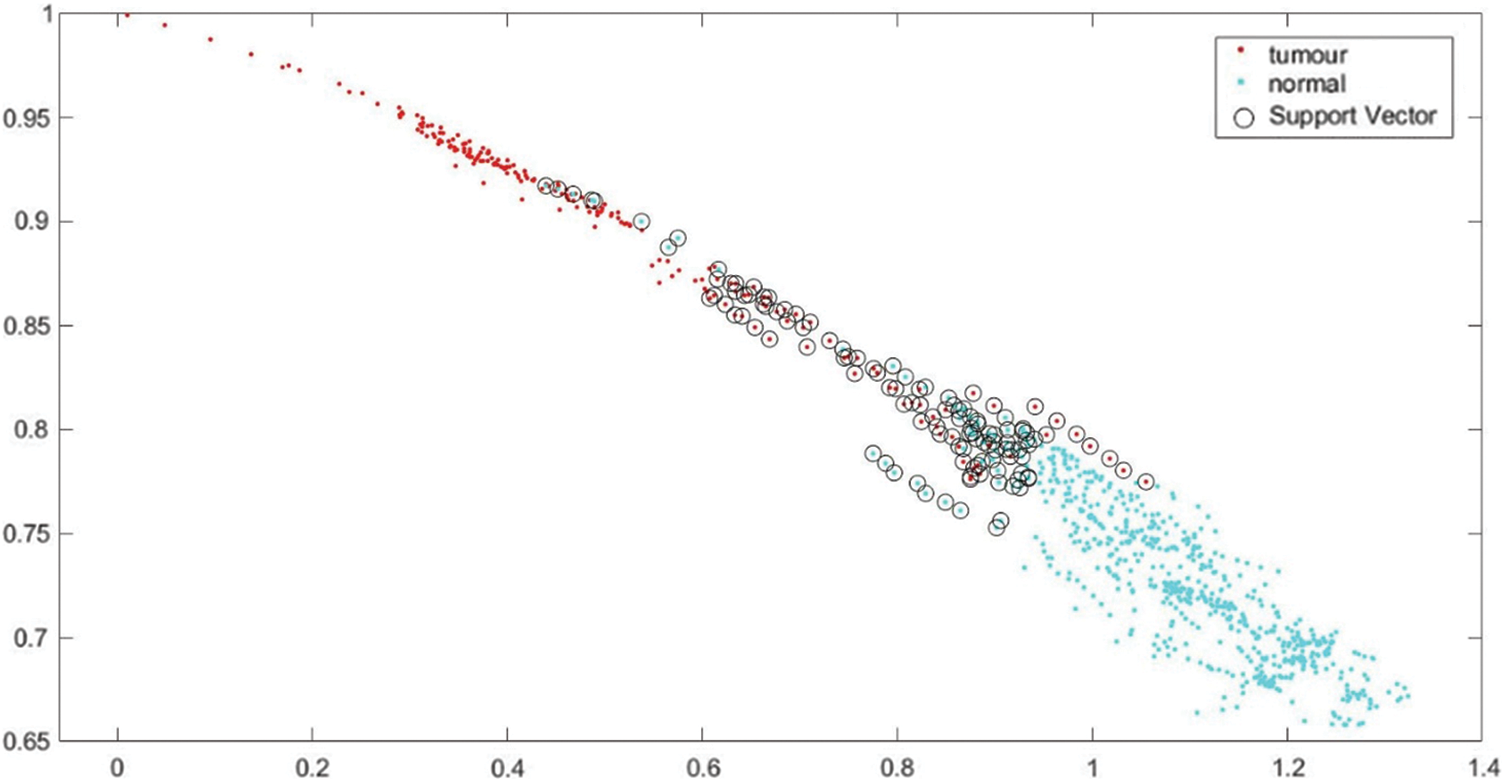
Figure 8: SVM class labels and support vectors
4.1.2 Method B-Classification Using Proposed CNN
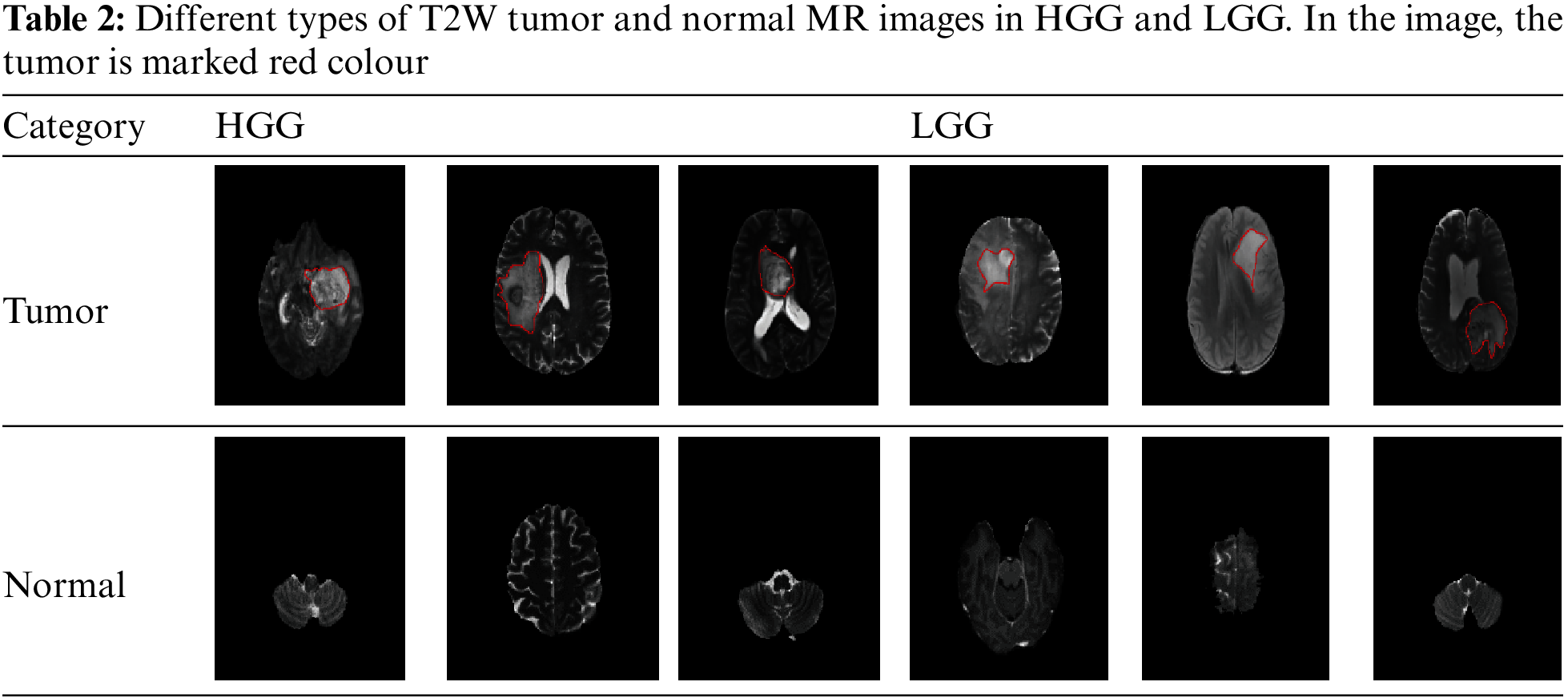
The classification process using convolutional neural networks (CNN) is a combination of pre-trained, feedforward, and fully connected neural networks. Similar Method A images are also utilized for classification, encompassing both normal and tumor images. The tumor can occur in various locations within the brain. Examples of normal images and images depicting different locations where the tumor can manifest are provided in Table 2.
The established CNN classification approach consists of two main components: feature extraction and classification. The feature extraction part includes the input layer, convolutional layer, and pooling layers. On the other hand, the classification part involves the output layers and fully connected layers. The input layer receives tumor and normal images as input, with a size of 240 × 240 × 1. The convolution layer is applied initially, followed by batch normalization and rectified linear unit (ReLU) layers within the network. The pooling layer utilizes max-pooling, which reduces the output size by half compared to the input. The fully connected layers gather information from these smaller parts for classification. Finally, the output layer generates the output image. This CNN classification network technique comprises a total of nineteen layers, including input, hidden, and output layers.
The proposed method utilizes an input layer with an image size of
The network training process incorporates an image input layer to accept the input images. The convolutional layers form the core of the neural network. These layers take the input image and convolve it with a set of filters to extract features and generate a feature map. The filters are represented by M (i, j), and the image by N (i, j). To standardize the input and accelerate training, a batch normalization layer is applied. Subsequently, a ReLU layer is used as an activation function to capture only positive values, returning 0 for any negative values. A max-pooling layer is utilized to select the maximum value within a region of the feature map. Additionally, a fully connected layer, which is a feed-forward network, collects input data from the final pooling layers.
The SoftMax layer serves as an activation function to normalize the outputs. Finally, a classification layer computes weighted classification tasks, employing mutually exclusive tasks and cross-entropy loss for classification. The network is trained using stochastic gradient descent with momentum (sgdm) [42]. By incorporating a momentum term, sgdm overcomes the oscillation issues of standard stochastic gradient descent. The layer-wise workflow of the proposed CNN classification network is illustrated in Fig. 9.
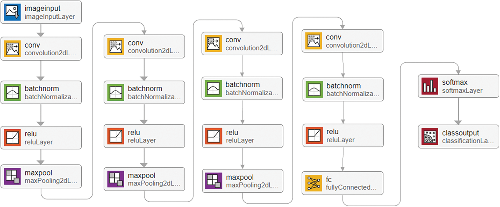
Figure 9: Layer-wise proposed CNN classification network workflow
The neural network classification in this approach was conducted using MATLAB R2021a (academic version) and relied on a single CPU for hardware resources. A fixed learning rate of 0.01 was employed, and the learning rate schedule remained constant throughout. The training process consisted of ten epochs, each with three iterations, resulting in a total of thirty iterations. Upon reaching Epoch 10, the training was automatically terminated. Accuracy, represented by the color blue, and loss, denoted by the color red, were computed and evaluated. The training process for the 45,756 images was completed in 3 min and 35 s. The training progress of the developed CNN classification method is illustrated in Fig. 10.
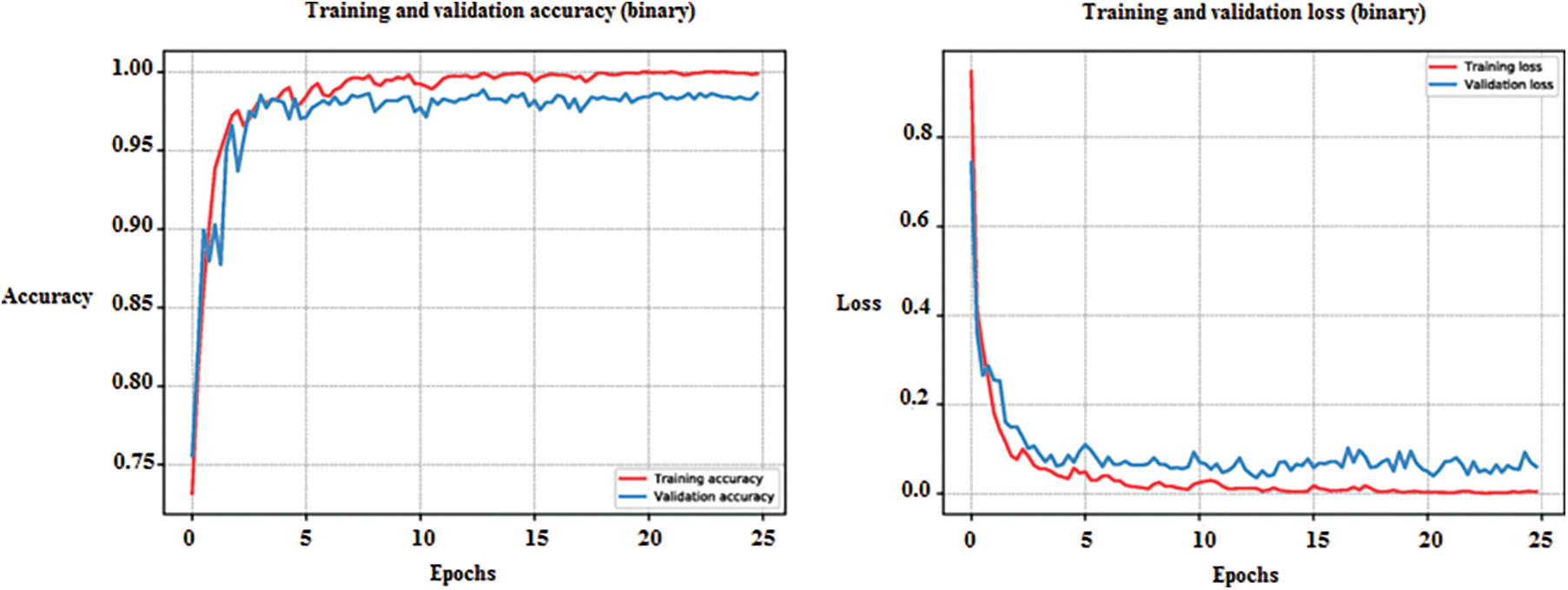
Figure 10: Training progress of developed method of CNN classification
4.1.3 Compare the Classification Results
In this paper, two classification methods were employed: Method A-the GLCM method, and Method B-the proposed CNN method. Both methods exclusively utilized T2W-MR images for training and testing purposes. During the training and testing processes, both techniques extracted features from the images. The confusion matrix was used to evaluate the classification results, with class labels “normal” (0) and “tumor” (1) being indicated. The rows of the matrix represent the true class labels, while the columns represent the predicted class labels. The confusion matrix results for Method A and Method B methods are illustrated in Fig. 11.
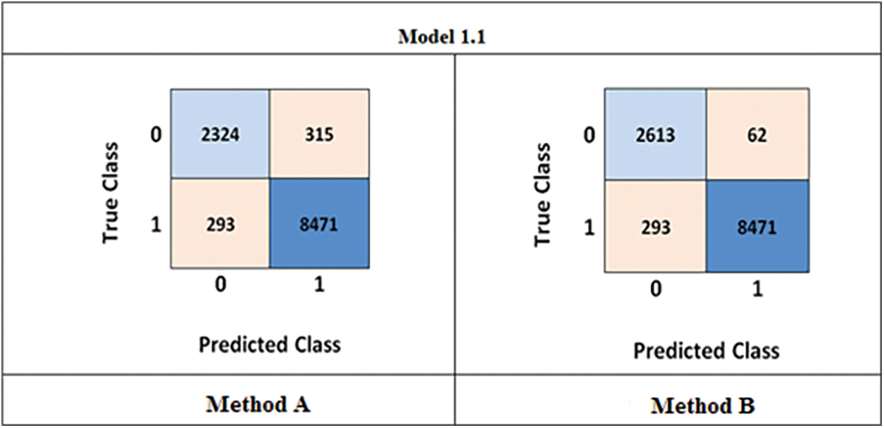
Figure 11: Confusion matrix (Method-A) GLCM method (Method-B) developed CNN
Upon comparing the results obtained from the above confusion matrix, it can be observed that the GLCM method had a higher number of incorrect classifications, with 351 normal images being classified as tumors. On the other hand, the proposed method exhibited a lower number of incorrect classifications, with only 62 normal images being misclassified as tumors. Additionally, the accuracy, sensitivity, and specificity were calculated using Eqs. (1) to (3) as mentioned earlier. The Method A achieved an accuracy, sensitivity, and specificity of 94.87%, 89.77%, and 96.35%, respectively, while the Method B achieved 99.65%, 90.81%, and 97.43%, respectively. Based on these results, it can be concluded that the proposed CNN method yields superior outcomes.
Segmentation of brain tumors plays a crucial role in identifying tumor regions within MRI scans. This process divides the MR images into three distinct parts: Tumor Core (TC), Enhanced Tumor (ET), and Whole Tumor (WT). In the BraTS 2020 dataset, each patient image is assigned a unique sequence number. In the preceding Method B-proposed CNN classification section, a specific T2W image is classified as a tumor, leading to the consideration of all other MRI multimodal images such as T1W, FLAIR, and T1C as tumor images as well. FLAIR, among all the multimodal images, clearly delineates the entire tumor, whereas T1W has limitations in spatial resolution and contrast and exhibits heterogeneous tissue characteristics. However, T1W provides a distinct boundary for the tumor core and enhanced tumor. It is crucial to consider the specific requirements of the segmentation task, the clinical context, and the available data when choosing the imaging modality and sequence. In some cases, T1W and T2W images alone may suffice, while in others, incorporating additional image types can enhance segmentation accuracy and clinical utility. Therefore, this segmentation method utilizes FLAIR and T1W images.
U-Net, a convolutional neural network (CNN), was originally developed in 2015 by the Computer Science Department at the University of Freiburg specifically for medical image segmentation [43]. This network was designed to achieve accurate segmentation even with limited training images and is based on a fully convolutional network [44]. In this study, a modified U-Net architecture is proposed for segmentation purposes using the same MATLAB R2021a (academic version). The input for segmentation consists of FLAIR and T1C images. The FLAIR image is provided with two class labels: background and whole tumor, while the T1C image is given three class labels: background, enhanced tumor, and tumor core.
The proposed method comprises two crucial components: the encoder component (down-sampling) and the decoder component (up-sampling), with a bridge section connecting the two. The term “Encoder Depth” is used to indicate the depth of both the up-sampling and down-sampling subnetworks. If the encoder depth is denoted as N, then both the encoder and decoder parts consist of N blocks, making the U-Net a symmetric network [45]. In this modified U-Net architecture, the Encoder Depth is set to four, resulting in four blocks in both the encoder and decoder parts, with each block consisting of five layers. Additionally, a residual block is employed in all encoder layers to transform low-level features into high-level features and enhance segmentation results.
In each encoder block, the first four layers consist of two sets of convolutional and ReLU layers, while the final layer is a max-pool layer. The decoder blocks, on the other hand, start with a transposed convolutional layer as the primary layer, followed by two sets of convolutional and ReLU layers in the subsequent four layers. The encoder blocks gather features from the input image in the first four layers and reduce the size in the last layer, transforming the image from
During the concatenation process, only blocks of the same size from the up-sampling and down-sampling processes are concatenated. In the encoder blocks, the convolutional layers use 64, 128, 512, and 1024 num-filters, with a filter size of
For each pixel in the image, the U-Net architecture employs a loss function that aids in the precise identification of individual pixels within the segmentation map. The choice of loss function and network structure significantly impacts the performance of neural networks [40]. In this proposed method, which involves segmenting multiple classes within brain tumors, a multiclass dice loss function is utilized. The modified U-Net architecture of the proposed method is depicted in Fig. 12.
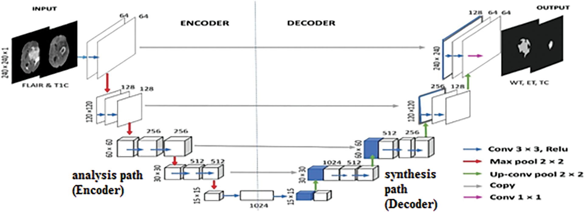
Figure 12: The proposed method comprises two crucial components: the encoder component (down-sampling) and the decoder component (up-sampling), with a bridge section connecting the two modified U-Net architecture
This section presents the segmentation of brain tumors using an efficient modified U-Net (EMU-Net) architecture, and the results are validated from various perspectives. The segmentation process is performed twice: firstly, the FLAIR images are segmented into the background and the whole tumor, and then the T1C images are segmented into the background, enhanced tumor, and tumor core. The dataset used includes HGG and LGG-type images from the dataset. These segmentation components are combined to generate the complete tumor image, and the results are evaluated using the Dice Similarity Coefficient (DSC) measure, compared to the ground truth image.
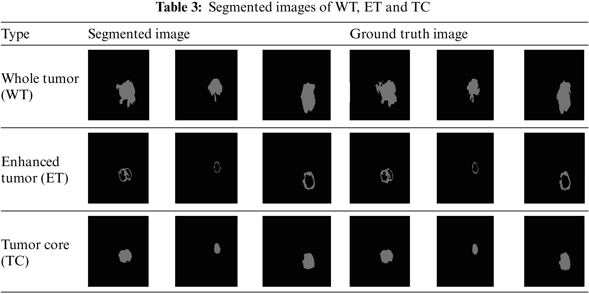
For the classification task, this method utilized 11,439 patient images, and the Method B proposed CNN method successfully classified 2,613 images as having tumors (1). Therefore, the same set of 2,613 FLAIR and T1C images is employed for the segmentation task. During the training process, all FLAIR and T1C images are provided as input to the proposed modified U-Net architecture. The architecture segments the tumor regions, and these segmentation results are stored within the network. Subsequently, new FLAIR and T1C images are tested, and the technique automatically performs segmentation of the tumor regions based on the learned knowledge from the training phase. Table 3 presents the segmentation outcomes alongside the corresponding ground truth images.
The objective of the proposed network is to perform the segmentation of MR images into Tumor Core (TC), Enhanced Tumor (ET), and Whole Tumor (WT). This network receives two types of inputs: the original image and the labeled image. The dataset is divided into training, validation, and testing sets, with proportions of 60%, 20%, and 20%, respectively. The class labels include background (BG), WT, ET, and TC. Stochastic gradient descent with momentum is used in the training options, with a learning rate drop period set to 10, a starting learning rate of 0.001, the momentum of 0.9, a learning rate drop factor of 0.3, and a mini-batch size of 8.
The training process consists of 10 epochs, with an automatic shuffling of the data after each epoch. During training, the network learns from 60% of the training images and their corresponding class labels. The remaining images are used for validation and testing. The network training and testing are performed using a single CPU. Each epoch comprises ten iterations, resulting in a total of 100 iterations (10 epochs × 10 iterations). The final state is reached at the tenth epoch. The overall training duration is 2 min and 12 s. Accuracy and loss percentages are calculated to evaluate the performance of the developed method. The results are assessed using the Dice Similarity Coefficient (DSC) metric and compared with state-of-the-art methods. The test data results are presented in Table 4.
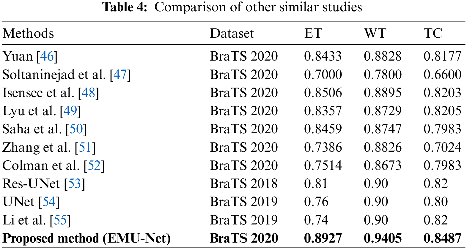
The comparison of Dice Similarity Coefficient (DSC) results reveals that the proposed method achieves a high DSC score for the whole tumor region but a relatively lower score for the enhanced tumor region. This discrepancy can be attributed to the fact that FLAIR images provide a more accurate boundary for the whole tumor area, while T1C images present a more complex boundary for the tumor core and enhanced tumor areas.
In comparison to Yuan’s method [46] for the enhanced tumor region, our proposed method utilizes a dynamic scale attention network with skip connections and long-range connections. Additionally, it employs a learning rate of 0.3 in conjunction with ResNet, which establishes connections only with important networks. When compared to Soltaninejad et al.’s method [47], our approach outperforms all tumor sub-regions due to its utilization of a smaller field of view for segmentation and the incorporation of a coarse down-sampling path. The DSC results of the proposed method, in comparison with state-of-the-art techniques, are illustrated in Fig. 13.
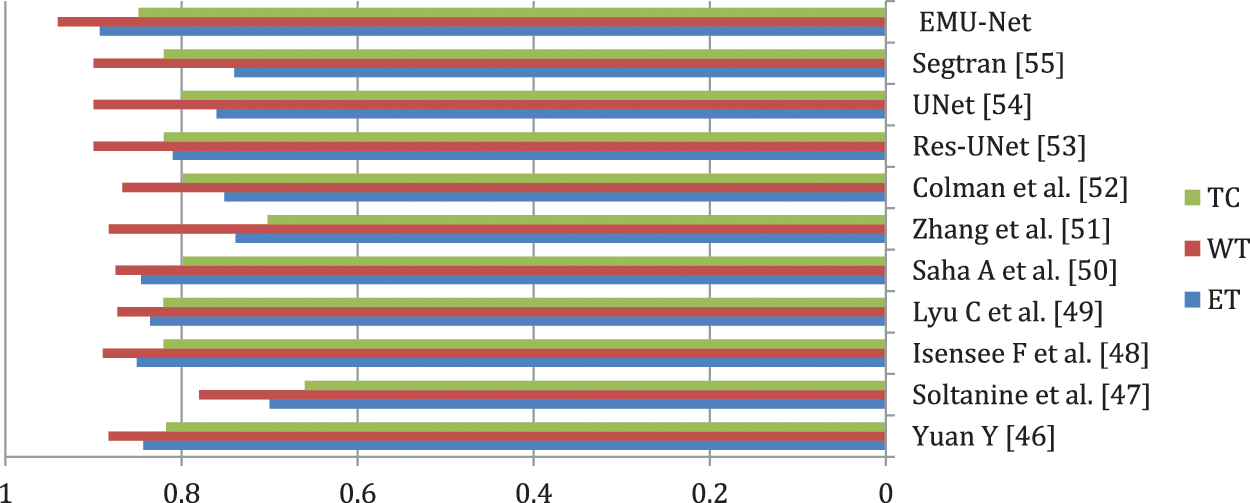
Figure 13: Proposed method DSC results
In the comparison to Isensee et al. [48], the proposed method demonstrates superior performance in segmenting the tumor core and enhanced tumor regions. It utilizes a modified U-Net architecture for segmentation and employs an expanded batch size strategy to enhance the network’s understanding of tumorous areas. Notably, it achieves an impressive DSC score of 0.8487 for the enhanced tumor region.
Overfitting is a common challenge in U-Net segmentation, which Lyu et al. [49] address by incorporating variational autoencoder regularization in both the encoding and decoding phases. By leveraging an expanded dataset, this approach utilizes network adapt attention gates and additional training, leading to accurate predictions of the enhanced tumor region and consequently yielding excellent DSC results.
In the study of Saha et al. [50], the primary objective is to achieve accurate segmentation. They incorporate a residual network in both the encoding and decoding stages, particularly emphasizing the utilization of a multi-pathway technique. While this method delivers average results across all tumor regions, it lacks the use of individual encoders for each stage and instead employs a common encoder for all stages.
Addressing the issue of voxel imbalance, Zhang et al. [51] employed different weights for different segment regions simultaneously. They introduce a new categorical dice loss function, which yields improved results for the whole tumor region. However, when compared to our proposed method, their approach exhibits a lower DSC score.
Similarly, in the study conducted by Colman et al. [52], their method achieves a high score solely for the whole tumor region. They utilize a deep residual network with 104 convolutional layers and employ a sparse categorical cross-entropy loss function. In contrast, our proposed method utilizes a multiclass dice loss function and focuses on all classes to prevent the loss, resulting in the best DSC results.
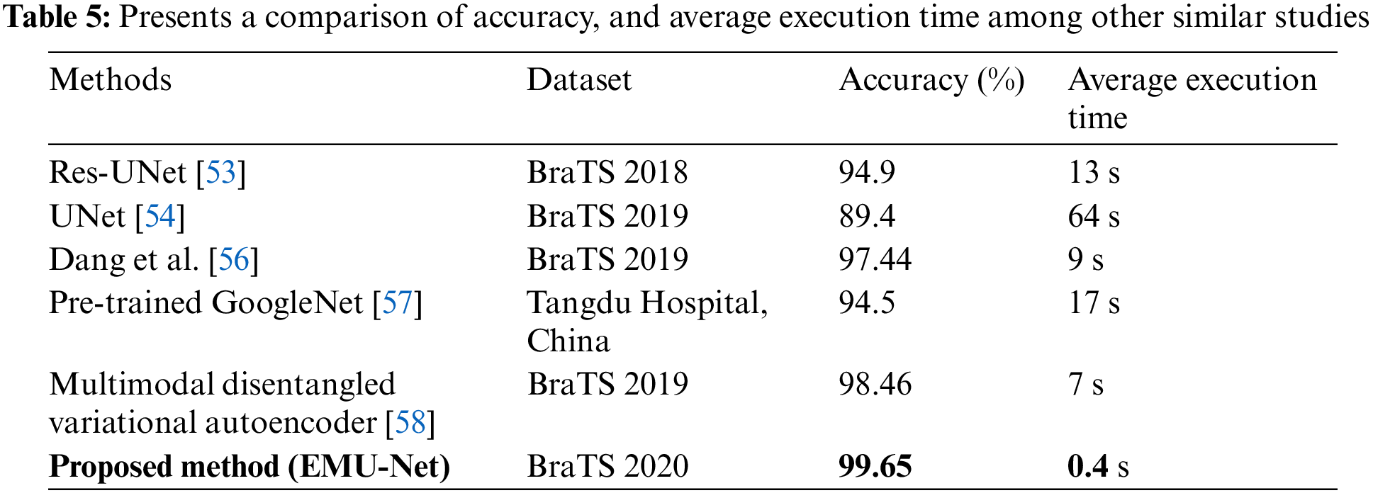
In Table 4, the performance of other studies that primarily concentrate on the BraTS dataset is compared. Our proposed pipeline demonstrates exceptional results in predicting TC, WT, and ET. Moreover, it substantially improves the Dice coefficient for TC, WT, and ET compared to the other studies. On the other hand, alternative designs like Res-UNet [53] showcase their effectiveness in enhancing tumor-core prediction.
Table 5 provides an overview of cutting-edge techniques that should be acknowledged for their exceptional accuracies, particularly [58]. The approach taken in their study for problem investigation can serve as a valuable reference for future research. The researchers in [58] devised an auto-encoder to reconstruct features derived from MRI images, encompassing intensity, wavelet, Laplacian of Gaussian, and local binary pattern. These features were then combined through two hidden layers to obtain the final prediction outcomes. Through an examination of other studies, it becomes evident that our method, EMU-Net, warrants further exploration and assessment in terms of extrapolation and generalization. EMU-Net enhance the low-level features by adding additional residual blocks to all encoder path layers, transforming them into high-level features. This modification leads to improved segmentation results. According to Table 5, the proposed technique demonstrates the lowest average computation time when compared to similar studies. Table 5 clearly indicates that the proposed model exhibits the fastest computation time along with the highest accuracy. The results indicate that the suggested method yielded precise and efficient segmentation outcomes. The time required to test a single image is unpredictable due to its brevity and occasional lack of accuracy. Consequently, the average number of test images per second is determined by conducting 300 MRI segmentation tasks on the BraTS19 and BraTS20 datasets.
The results of the experimented models, including the specific hyperparameters and configurations, are presented in Table 6. The models were trained using an initial learning rate of 0.01 for a total of 10 epochs. The Adam optimizer was utilized to enhance the detector performance, and the Dice loss function was employed.
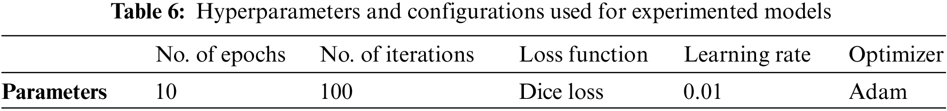
Fig. 14 depicts the comparison between the segmentation results and the ground truth for five distinct types of tumors using different models. In the figure, the red region represents glioma tumors, the green region represents meningioma tumors, and the yellow region represents pituitary tumors. In the segmentation figure of the Pre-Trained GoogleNet [57], certain glioma tumors are inaccurately identified as meningioma tumors, resulting in a triangular segmentation pattern that significantly differs from the ground truth. The U-Net model, on the other hand, demonstrates poor performance as it barely segments the tumor, yielding unsatisfactory results. The segmentation map produced by the Multimodal disentangled variational autoencoder [58] exhibits incorrect classification in nearly 50% of the regions, while the segmentation results from other models appear excessively smooth, despite correctly predicting the tumor categories. Conversely, the segmentation map by Dang et al. [56] performs poorly, displaying considerable deviation from the ground truth. In contrast, the proposed method (EMU-Net) achieves the best segmentation results with minimal error predictions, and notably superior edge segmentation effects compared to other models. The experimental results clearly demonstrate the robustness of the proposed method (EMU-Net) on the brain tumor dataset presented in this paper.
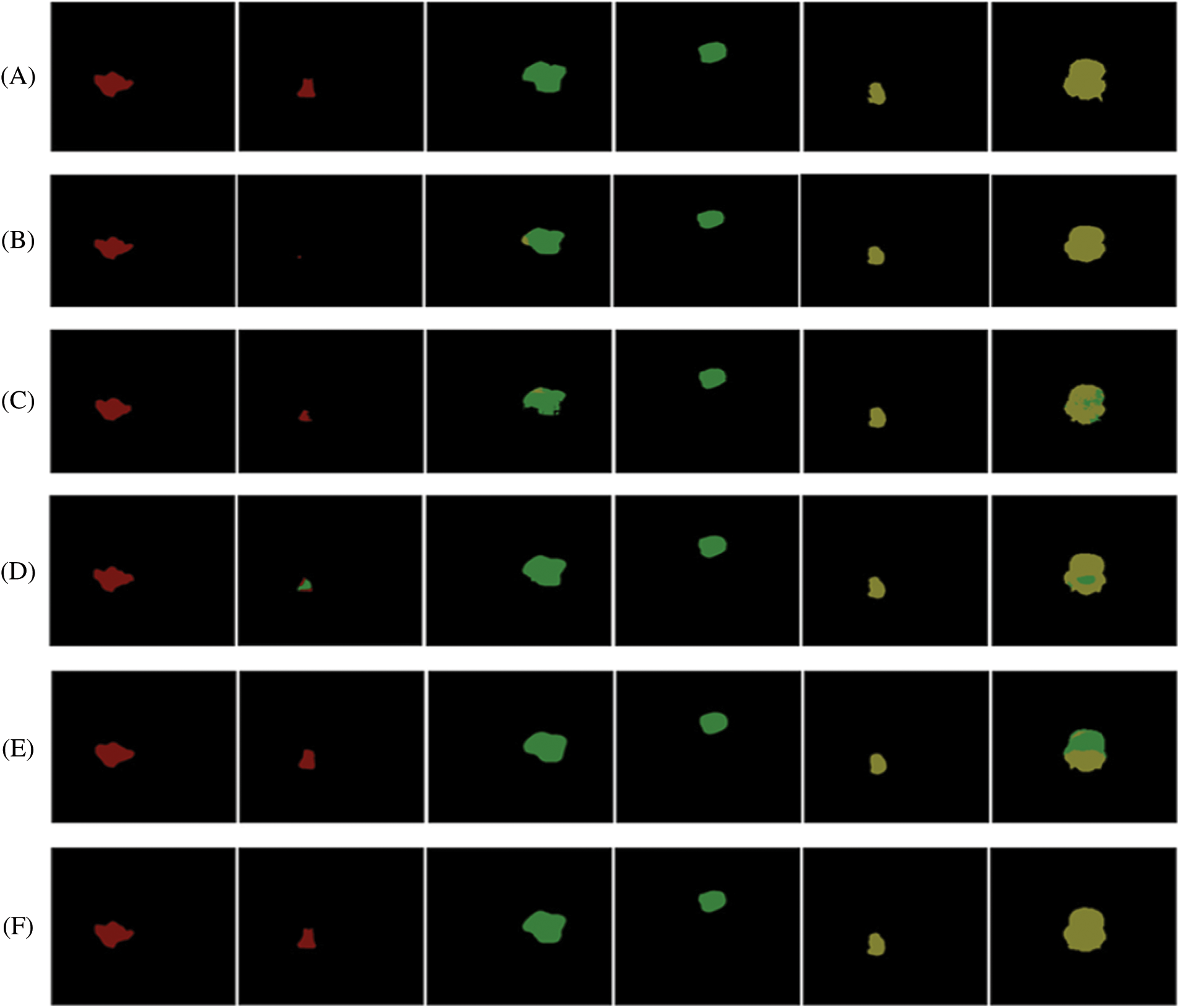
Figure 14: illustrates a comparison of segmentation results for different types of tumors obtained using various networks. The images are labeled as follows: (A) ground truth, (B) U-NeT, (C) Dang et al. [56], (D) Pre-trained GoogleNet [57], (E) Multimodal disentangled variational autoencoder [58], and (F) Proposed method (EMU-Net)
This paper utilizes BraTS2020 MRI multimodal images for both classification and segmentation purposes. The classification task involves two methods: Method A-GLCM method and Method B-proposed CNN. Only the T2W images are used for classification, and upon comparing the results, the Method B-proposed CNN method achieves an accuracy of 99.65%.
Following the classification, the classified tumor images are subjected to segmentation using the proposed modified U-Net architecture. The segmentation process specifically employs the FLAIR and T1C images. The segmentation results are evaluated using the DSC metric, yielding DSC scores of 0.8927, 0.9405, and 0.8487 for the tumor core, whole tumor, and enhanced tumor regions, respectively.
Moving forward, the goal is to enhance the performance of the proposed model and assess its effectiveness on additional benchmark datasets in the future. The outcomes of our study offer significant insights and recommendations for future CNN research. Our findings can be compared to the current leading methods in the field. Considering its remarkable overall accuracy, it is necessary to replicate the proposed study on a larger scale before applying it to other healthcare applications. This study establishes the groundwork for integrating CNN into the diagnosis of brain tumor segmentation, showcasing its advantages of speed, efficiency, and technological optimization. These attributes are particularly valuable during pandemics as they align with social distancing requirements. The proposed technique demonstrates the lowest average computation time when compared to similar studies. It is clear that the proposed model exhibits the fastest computation time along with the highest accuracy. By analyzing various studies, it becomes clear that our approach, EMU-Net, requires further investigation and evaluation regarding its extrapolation and generalization capabilities. EMU-Net enhances the low-level features by incorporating extra residual blocks into all encoder path layers, thereby transforming them into high-level features. This modification results in enhanced segmentation outcomes. The proposed method consists of two important elements: an encoder component responsible for down-sampling and a decoder component responsible for up-sampling. These components are based on a modified U-Net architecture and are connected by a bridge section.
Acknowledgement: The authors also gratefully acknowledge the helpful comments and suggestions of the reviewers, which have improved the presentation.
Funding Statement: Self-funded; no external funding is involved in this study.
Author Contributions: Conceptualization, M.A.; methodology, M.A.; formal analysis, M.A.; investigation, M.A. and A.S.A.; data curation, A.S.A. and M.A.; software, M.A.; writing—original draft preparation, M.A. and A.S.A.; writing—review and editing, M.A.; visualization, A.S.A. All authors have read and agreed to the published version of the manuscript.
Availability of Data and Materials: Data generated or analyzed during this study are available from the corresponding author upon reasonable request.
Conflicts of Interest: The authors declare that they have no conflicts of interest to report regarding the present study.
References
1. E. Irmak, “Multi-classification of brain tumor MRI images using deep convolutional neural network with fully optimized framework,” Iranian Journal of Science and Technology, Transactions of Electrical Engineering, vol. 45, no. 3, pp. 1015–1036, 2021. [Google Scholar]
2. F. E. Bleeker, J. Molenaar and S. Leenstra, “Recent advances in the molecular understanding of glioblastoma,” Journal of Neuro-Oncology, vol. 108, no. 1, pp. 11–27, 2012. [Google Scholar] [PubMed]
3. T. Magadza and S. Viriri, “Deep learning for brain tumor segmentation: A survey of state-of-the-art,” Journal of Imaging, vol. 7, no. 2, pp. 1–22, 2021. [Google Scholar]
4. S. Chen, C. Ding and M. Liu, “Dual-force convolutional neural networks for accurate brain tumor segmentation,” Pattern Recognition, vol. 88, no. suppl_5, pp. 90–100, 2019. [Google Scholar]
5. N. Gordillo, E. Montseny and P. Sobrevilla, “State of the art survey on MRI brain tumor segmentation,” Magnetic Resonance Imaging, vol. 31, no. 8, pp. 1426–1438, 2013. [Google Scholar] [PubMed]
6. W. Chen, B. Liu, S. Peng, J. Sun and X. Qiao, “S3D-UNet: Separable 3D U-Net for brain tumor segmentation,” in Brainlesion: Glioma, Multiple Sclerosis, Stroke and Traumatic Brain Injuries. Granada, Spain: Springer International Publishing, pp. 358–368, 2019. [Google Scholar]
7. M. A. Mazurowski, M. Buda, A. Saha and M. R. Bashir, “Deep learning in radiology: An overview of the concepts and a survey of the state of the art with focus on MRI,” Journal of Magnetic Resonance Imaging, vol. 49, no. 4, pp. 939–954, 2019. [Google Scholar] [PubMed]
8. A. Abdulkadir, O. Çiçek, S. S. Lienkamp and T. Brox, “3D U-Net: Learning dense volumetric segmentation from sparse annotation,” in Medical Image Computing and Computer-Assisted Intervention–MICCAI, Athens, Greece, pp. 17–21, 2016. [Google Scholar]
9. J. Shao, S. Chen, J. Zhou, H. Zhu and Z. Wang, “Application of U-Net and optimized clustering in medical image segmentation: A review,” Computer Modeling in Engineering & Sciences, vol. 136, no. 3, pp. 2173–2219, 2023. [Google Scholar]
10. S. Pereira, A. Pinto, V. Alves and C. A. Silva, “Brain tumor segmentation using convolutional neural networks in MRI images,” IEEE Transactions on Medical Imaging, vol. 35, no. 5, pp. 1240–1251, 2016. [Google Scholar] [PubMed]
11. J. Chen, Z. He, D. Zhu, B. Hui and R. Yi, “Mu-Net: Multi-path upsampling convolution network for medical image segmentation,” Computer Modeling in Engineering & Sciences, vol. 131, no. 1, pp. 73–95, 2022. [Google Scholar]
12. S. Hussain, S. M. Anwar and M. Majid, “Brain tumor segmentation using cascaded deep convolutional neural network,” in Annual Int. Conf. of the IEEE Engineering in Medicine and Biology Society (EMBC), Jeju, Korea (Southpp. 1998–2001, 2017. [Google Scholar]
13. S. Iqbal, M. U. Ghani, T. Saba and A. Rehman, “Brain tumor segmentation in multi-spectral MRI using convolutional neural networks (CNN),” Microscopy Research and Technique, vol. 81, no. 4, pp. 419–427, 2018. [Google Scholar] [PubMed]
14. G. Wang, W. Li, S. Ourselin and T. Vercauteren, “Automatic brain tumor segmentation using convolutional neural networks with test-time augmentation,” in Brainlesion: Glioma, Multiple Sclerosis, Stroke and Traumatic Brain Injuries. Granada, Spain: Springer International Publishing, pp. 61–72, 2019. [Google Scholar]
15. M. M. Thaha, K. P. M. Kumar and B. S. Murugan, “Brain tumor segmentation using convolutional neural networks in MRI images,” Journal of Medical Systems, vol. 43, no. 9, pp. 1–10, 2019. [Google Scholar]
16. R. Thillaikkarasi and S. Saravanan, “An enhancement of deep learning algorithm for brain tumor segmentation using kernel based CNN with M-SVM,” Journal of Medical Systems, vol. 43, no. 4, pp. 1–7, 2019. [Google Scholar]
17. Z. Zhou, Z. He and Y. Jia, “AFPNet: A 3D fully convolutional neural network with atrous-convolution feature pyramid for brain tumor segmentation via MRI images,” Neurocomputing, vol. 402, no. 11, pp. 235–244, 2020. [Google Scholar]
18. R. A. Zeineldin, M. E. Karar and J. Coburger, “DeepSeg: Deep neural network framework for automatic brain tumor segmentation using magnetic resonance flair images,” International Journal of Computer Assisted Radiology and Surgery, vol. 15, no. 6, pp. 909–920, 2020. [Google Scholar] [PubMed]
19. T. Kalaiselvi, S. T. Padmapriya, P. Sriramakrishnan and K. Somasundaram, “Deriving tumor detection models using convolutional neural networks from MRI of human brain scans,” International Journal of Information Technology, vol. 12, no. 2, pp. 403–408, 2020. [Google Scholar]
20. H. Chen, Z. Qin, Y. Ding, L. Tian and Z. Qin, “Brain tumor segmentation with deep convolutional symmetric neural network,” Neurocomputing, vol. 392, no. 6, pp. 305–313, 2020. [Google Scholar]
21. S. Vijh, S. Sharma and P. Gaurav, “Brain tumor segmentation using OTSU embedded adaptive particle swarm optimization method and convolutional neural network,” in Data Visualization and Knowledge Engineering: Spotting Data Points with Artificial Intelligence, vol. 32. Barcelona, Spain: Springer, pp. 171–194, 2020. [Google Scholar]
22. S. Preethi and P. Aishwarya, “Combining wavelet texture features and deep neural network for tumor detection and segmentation over MRI,” Journal of Intelligent Systems, vol. 28, no. 4, pp. 571–588, 2019. [Google Scholar]
23. W. Widhiarso, Y. Yohannes and C. Prakarsah, “Brain tumor classification using gray level co-occurrence matrix and convolutional neural network,” Indonesian Journal of Electronics and Instrumentation Systems, vol. 8, no. 2, pp. 179–190, 2018. [Google Scholar]
24. A. R. Munajat and F. Utaminingrum, “Brain tumor detection system based on sending email using gray level co-occurrence matrix and back-propagation neural network,” in Proc. of Int. Conf. on Sustainable Information Engineering and Technology, New York, USA, pp. 321–326, 2021. [Google Scholar]
25. M. Z. Alom, C. Yakopcic, T. M. Taha and V. K. Asari, “Recurrent residual convolutional neural network based on U-Net (R2U-Net) for medical image segmentation,” in NAECON. IEEE National Aerospace and Electronics Conf., Dayton, USA, pp. 228–233, 2018. [Google Scholar]
26. Z. Zhang, Q. Liu and Y. Wang, “Road extraction by deep residual U-Net,” IEEE Geoscience and Remote Sensing Letters, vol. 15, no. 5, pp. 749–753, 2018. [Google Scholar]
27. F. Milletari, N. Navab and S. A. Ahmadi, “Fully convolutional neural networks for volumetric medical image segmentation,” in 4th IEEE Int. Conf. on 3D Vision (3DV), Stanford, USA, pp. 565–571, 2016. [Google Scholar]
28. S. S. M. Salehi, D. Erdogmus and A. Gholipour, “Auto-context convolutional neural network (auto-net) for brain extraction in magnetic resonance imaging,” IEEE Transactions on Medical Imaging, vol. 36, no. 11, pp. 2319–2330, 2017. [Google Scholar]
29. Z. Zhou, M. M. R. Siddiquee, N. Tajbakhsh and J. Liang, “UNet++: Redesigning skip connections to exploit multiscale features in image segmentation,” IEEE Transactions on Medical Imaging, vol. 39, no. 6, pp. 1856–1867, 2019. [Google Scholar] [PubMed]
30. W. Chen, Y. Zhang, J. He, Y. Qiao, Y. Chen et al., “Prostate segmentation using 2D bridged U-Net,” in Int. Joint Conf. on Neural Networks, Budapest, Hungary, pp. 1–7, 2019. [Google Scholar]
31. M. Naser and M. Deen, “Brain tumor segmentation and grading of lowergrade glioma using deep learning in MRI images,” Computers in Biology and Medicine, vol. 121, pp. 1–12, 2020. [Google Scholar]
32. S. Bakas, M. Reyes, A. Jakab, S. Bauer, M. Rempfler et al., “Identifying the best machine learning algorithms for brain tumor segmentation,” arXiv preprint arXiv:1811.02629, 2018. [Google Scholar]
33. B. H. Menze, A. Jakab, S. Bauer, J. Kalpathy-Cramer, K. Farahani et al., “The Multimodal Brain Tumor Image Segmentation Benchmark (BRATS),” IEEE Transactions on Medical Imaging, vol. 34, no. 10, pp. 1993–2024, 2015. [Google Scholar]
34. E. Elsayed and M. Aly, “Hybrid between ontology and quantum particle swarm optimization for segmenting noisy plant disease image,” International Journal of Intelligent Engineering and Systems, vol. 12, no. 5, pp. 299–311, 2019. [Google Scholar]
35. M. Aly and N. S. Alotaibi, “A novel deep learning model to detect COVID-19 based on wavelet features extracted from Mel-scale spectrogram of patients’ cough and breathing sounds,” Informatics in Medicine Unlocked, vol. 32, no. 1, pp. 1–11, 2022. [Google Scholar]
36. M. Aly and N. S. Alotaibi, “A new model to detect COVID-19 coughing and breathing sound symptoms classification from CQT and Mel spectrogram image representation using deep learning,” International Journal of Advanced Computer Science and Applications, vol. 13, no. 8, pp. 601–611, 2022. [Google Scholar]
37. M. Aly and A. S. Alotaibi, “Molecular property prediction of modified gedunin using machine learning,” Molecules, vol. 28, no. 3, pp. 1–15, 2023. [Google Scholar]
38. P. Mohanaiah, P. Sathyanarayana and L. GuruKumar, “Image texture feature extraction using GLCM approach,” International Journal of Scientific and Research Publications, vol. 3, no. 5, pp. 1–5, 2013. [Google Scholar]
39. B. Dunn, M. Pierobon and Q. Wei, “Automated classification of lung cancer subtypes using deep learning and CT-scan based radiomic analysis,” Bioengineering, vol. 10, no. 6, pp. 1–16, 2023. [Google Scholar]
40. C. H. Sudre, W. Li, T. Vercauteren, S. Ourselin and M. J. Cardoso, “Generalised dice overlap as a deep learning loss function for highly unbalanced segmentations,” in Deep Learning in Medical Image Analysis and Multimodal Learning for Clinical Decision Support. Canada: Québec City, pp. 240–248, 2017. [Google Scholar]
41. S. Taqvi, H. Zabiri, F. Uddin, M. Naqvi, L. D. Tufa et al., “Simultaneous fault diagnosis based on multiple kernel support vector machine in nonlinear dynamic distillation column,” Energy Science & Engineering, vol. 10, no. 3, pp. 814–839, 2022. [Google Scholar]
42. M. Ammar, M. E. Daho, K. Harrar and A. Laidi, “A feature extraction using cnn for peripheral blood cells recognition,” EAI Endorsed Transactions on Scalable Information Systems, vol. 9, no. 34, pp. 1–8, 2022. [Google Scholar]
43. O. Ronneberger, P. Fischer and T. Brox, “U-Net: Convolutional networks for biomedical image segmentation,” in Medical Image Computing and Computer-Assisted Intervention-MICCAI. Munich, Germany: Springer International Publishing, pp. 234–241, 2015. [Google Scholar]
44. E. Shelhamer, J. Long and T. Darrell, “Fully convolutional networks for semantic segmentation,” IEEE Transactions on Pattern Analysis and Machine Intelligence, vol. 39, no. 4, pp. 640–651, 2017. [Google Scholar] [PubMed]
45. M. Aghalari, A. Aghagolzadeh and M. Ezoji, “Brain tumor image segmentation via asymmetric/symmetric UNet based on two-pathway-residual blocks,” Biomedical Signal Processing and Control, vol. 69, no. 6, pp. 1–12, 2021. [Google Scholar]
46. Y. Yuan, “Automatic brain tumor segmentation with scale attention network,” in Brainlesion: Glioma, Multiple Sclerosis, Stroke and Traumatic Brain Injuries. Lima, Peru: Springer International Publishing, pp. 285–294, 2021. [Google Scholar]
47. M. Soltaninejad, T. Pridmore and M. Pound, “Efficient MRI brain tumor segmentation using multi-resolution encoder-decoder networks,” in Int. MICCAI Brainlesion Workshop, Lima, Peru, pp. 30–39, 2020. [Google Scholar]
48. F. Isensee, P. F. Jäger, P. M. Full, P. Vollmuth and K. H. Maier-Hein, “nnU-Net for brain tumor segmentation,” in Brainlesion: Glioma, Multiple Sclerosis, Stroke and Traumatic Brain Injuries. Lima, Peru: Springer International Publishing, pp. 118–132, 2021. [Google Scholar]
49. C. Lyu and H. Shu, “A two-stage cascade model with variational autoencoders and attention gates for MRI brain tumor segmentation,” in Brainlesion: Glioma, Multiple Sclerosis, Stroke and Traumatic Brain Injuries. Lima, Peru: Springer International Publishing, pp. 435–447, 2021. [Google Scholar]
50. A. Saha, Y. D. Zhang and S. C. Satapathy, “Brain tumor segmentation with a muti-pathway ResNet based UNet,” Journal of Grid Computing, vol. 19, no. 4, pp. 1–10, 2021. [Google Scholar]
51. W. Zhang, G. Yang, H. Huang, W. Yang, X. Xu et al., “ME-Net: Multi encoder net framework for brain tumor segmentation,” International Journal of Imaging Systems and Technology, vol. 31, no. 4, pp. 1834–1848, 2021. [Google Scholar]
52. J. Colman, L. Zhang, W. Duan and X. Ye, “DR-Unet104 for multimodal MRI brain tumor segmentation,” in Brainlesion: Glioma, Multiple Sclerosis, Stroke and Traumatic Brain Injuries. Lima, Peru: Springer International Publishing, pp. 410–419, 2021. [Google Scholar]
53. M. Noori, A. Bahri and K. Mohammadi, “Attention-guided version of 2D UNet for automatic brain tumor segmentation,” in 9th Int. Conf. on Computer and Knowledge Engineering (ICCKE), Mashhad, Iran, IEEE, pp. 269–275, 2019. [Google Scholar]
54. M. Decuyper, S. Bonte, K. Deblaere and R. van Holen, “Automated MRI based pipeline for segmentation and prediction of grade, IDH mutation and 1p19q co-deletion in glioma,” Computerized Medical Imaging and Graphics, vol. 88, pp. 1–10, 2021. [Google Scholar]
55. S. Li, X. Sui, X. Luo, X. Xu, Y. Liu et al., “Medical image segmentation using squeeze-and-expansion transformers,” arXiv preprint arXiv:2105.09511, 2021. [Google Scholar]
56. K. Dang, T. Vo, L. Ngo and H. Ha, “A deep learning framework integrating mri image preprocessing methods for brain tumor segmentation and classification,” International Brain Research Organization Neuroscience Reports, vol. 13, no. 12, pp. 523–532, 2022. [Google Scholar]
57. Y. Yang, L. Yan, X. Zhang, Y. Han, H. Nan et al., “Glioma grading on conventional mr images: A deep learning study with transfer learning,” Frontiers in Neuroscience, vol. 12, pp. 1–11, 2018. [Google Scholar]
58. J. Cheng, M. Gao, J. Liu, H. Yue, H. Kuang et al., “Multimodal disentangled variational autoencoder with game theoretic interpretability for glioma grading,” IEEE Journal of Biomedical and Health Informatics, vol. 26, no. 2, pp. 673–684, 2022. [Google Scholar] [PubMed]
Cite This Article
 Copyright © 2023 The Author(s). Published by Tech Science Press.
This work is licensed under a Creative Commons Attribution 4.0 International License , which permits unrestricted use, distribution, and reproduction in any medium, provided the original work is properly cited.
 Downloads
 Citation Tools