Traffic Flow Prediction with Heterogenous Data Using a Hybrid CNN-LSTM Model

1  Introduction

Traffic flow prediction is essential in intelligent transportation systems, as it plays a crucial role in numerous practical applications. Predicting traffic flow can help transportation managers reduce traffic congestion [1], one of the transportation industry’s most significant challenges. Congestion has several negative impacts, including longer travel times, noise pollution, air pollution, increased greenhouse gas emissions, and higher fuel consumption [2]. As urban communities continue to experience an increasing trend in-vehicle use yearly, addressing this problem will become more critical [3].

Many approaches for traffic flow prediction have been developed, categorized as parametric, non-parametric, and neural networks. Parametric methods such as ARIMA [4–9] and the Kalman Filtering model [10–14] function effectively with small amounts of data and data with linear characteristics. However, the majority of parametric techniques cannot account for variables such as variations and nonlinearity [15]. In contrast, a non-parametric approach, such as machine learning techniques, has been shown to aid in traffic flow forecasting. Support vector machine (SVM) and K-nearest neighbors (KNN) are the most often employed approaches for this purpose [16–18]. However, this method is to be more sensitive to noise or disturbances in the data. If the data has significant noise, non-parametric methods may produce inaccurate predictions. Non-parametric methods also often require selecting appropriate parameters to produce accurate predictions. If the selected parameters are inappropriate, the resulting predictions may be inaccurate.

The current Neural Networks methods for predicting time series, such as Artificial Neural Networks (ANN) [16,17,19], Feed-forward Neural Networks (FFNN) [20,21], Recurrent Neural Networks (RNN) [22–24], hybrid Recurrent Neural Network and Long short-term memory (RNN-LSTM) [24], Convolutional Neural Network (CNN) [2,25,26], and Long short-term memory (LSTM) [27,28] been used frequently. Deep learning and machine learning technologies [29] have demonstrated impressive success in fitting the detailed features of data and have drawn significant interest [30–32]. Nonetheless, the extant works based on deep learning models for traffic flow prediction have some limitations. Some works, such as the LSTM model, employ a simple neural network model that cannot completely capture the complex characteristics of traffic flow, resulting in a modest improvement in prediction performance.

Traffic flow prediction approaches that have been developed recently rely heavily on correlations between historical temporal and spatial data. However, in practice, research on traffic flow prediction has not involved much spatiotemporal data, which is believed to increase the performance of prediction results. Distribution and deployment of spatiotemporal data depend on location, and access is exceedingly limited. To overcome the limitations of spatiotemporal data, we explore the available data sources. Here we proposed three alternative spatiotemporal data features: vehicle type, holidays, and weather. We divide the vehicle traffic flow into five specific vehicle types (5 types). In addition, we also added holidays (3 types) and weather (10 conditions) for spatiotemporal data input. Hence, this work turns traffic data into pictures for processing, with the images represented by a matrix [33].

Handling the non-linear data abovementioned, we need a model that can extract meaningful information on spatiotemporal data and time-series information to enhance the precision of traffic flow prediction. CNN has a framework built specifically to handle data using a grid-like structure [33,34]. For instance, in the case of time series data, this can be conceptualized as a one-dimensional grid repeatedly sampled along the time vector. The information in a picture can be stored as a grid of pixels in two dimensions [2]. To efficiently manage data with a grid structure, CNN relies on a convolution kernel that can effectively extract features from the input. Incorporating sparse interactions, shared parameters, and equivariant representation, CNN has a higher capacity to comprehend data. On the other hand, LSTM models may be able to effectively capture sequence pattern information, which is the essential notion underlying its application to time-series problems.

To deal with the typical characteristics of spatiotemporal data, we propose the CNN-LSTM method that exploits the supremacy of CNNs for extracting spatial data to the fullest extent and the dominance of the LSTM network for extracting time-series information. This method captures possible correlations between variables and extracts composite features from a diverse input data set. To determine whether alternative models are superior, we conducted experiments with four models to compare and analyze: the LSTM, BILSTM, LSTM-BILSTM, and CNN-LSTM models. At the end of the investigation, the Mean absolute error (MAE), mean square error (MSE), and root mean square error (RMSE) are used to evaluate the model performance.

The following portions of the paper are organized as follows: The second section describes the research data. The third section provides the proposed method. The fourth section discusses the results of the experiment. The paper’s conclusion is located in the fifth section. Section sixth provides the research discussion.

2  Research Data

Research data was collected from various sources from November 2016 to October 2019 (three years). The raw resources of traffic flow data were downloaded from Taiwan’s open data platform, Traffic Data Collection System (TDCS) (https://tisvcloud.freeway.gov.tw/history/TDCS/M06A/) [35]. TDCS data is the vehicle trip record data on the Taiwan Freeway. After the data is downloaded, several steps are carried out to produce the expected traffic flow data.

Pre-processing vehicle trip record data can be complex due to different nations’ unique freeway electronic gantry systems. For example, Figs. 1a and 1b illustrate the trip logging and payment mechanisms for freeway electronic gantries in Taiwan and the United States, respectively. In the US, electronic gantries are installed at every intersection, which makes it easy to record vehicle trip start and end times. This system requires no additional work to extract traffic flow, but it can be more expensive due to the increased number of gantries.

Figure 1: (a) Taiwan freeway gantry system (b) US freeway gantry system

In contrast, Taiwan’s freeway gate system installs electronic gantries between intersections, reducing the necessary expenditures but complicating the collection of vehicle trip records in particular areas. With fewer electronic gantries, numerous possible combinations of trips occur, making it challenging to obtain information on them. For example, a sedan driver may only pass through one gate and exit at the next intersection, which does not meet the recording criteria in the research area segment. As a result, extracting traffic flow data from these records becomes more complicated.

In this paper, to overcome this complicated data extraction problem, a scalable approach developed in [35–37] is adapted to extract maximal repeats and class frequency distributions from gantry-timestamp sequential data with tags. A maximal repeat is a sequence of characters or patterns that appears more than once within a more extensive sequence and cannot be extended further without becoming a different sequence. Then, one can browse or inspect these classes’ frequency distributions of these gantry-timestamp maximal repeats to determine the regularities of vehicle travel time intervals among consecutive gantries according to periodic time intervals, e.g., 24 h/per day, weekday. In this study, each vehicle trip is represented as one gantry-timestamp sequence with tags, where tags include the type of vehicle and the metadata derived from the date of that trip. Fig. 2 shows the maximal repeat example. There were four maximal repeats, “MR_1”, “MR_2”, MR_3,” and “MR_4”, extracted from Fig. 1a. For example, the segment with the first three items “(GID_0+ “08:30”) (GID_1+ “08:33”) (GID_2+ “08:36”)” was always followed by the item “(GID_3+ “08:40”)”; the segment with last two items “(GID_6+ “08:50”) (GID_7+ “08:55”)” was preceded by the item “(GID_5+ “08:46”)”. While “MR_4” is the shortest maximal repeat because “(GID_4+ “08:43”)” is not always preceded by “(GID_3+ “08:40”)” and followed by “(GID_7+ “08:55)”.

Figure 2: (a) Five vehicle trips of tagged gantry-timestamp sequences. (b) Maximal repeats (Segment) extracted from Fig. 2a

In this study, we collect vehicle traffic flow data from eight electronic gantries on Taiwan’s National Freeway No. 3. Weather data is retrieved from open weather (https://openweathermap.org/), and holiday data is accessed from timeanddate.com (https://timeanddate.com). At this early stage, in the provided CNN-LSTM model, data extracting is conducted, followed by pre-processing step to standardize the input data in the range [0, 1] using the library from scikit-learn. This study uses 168 historical hours to forecast traffic data over the next 168 h (one week). The information on the vehicle type can be seen in Table 1. There are five types of vehicles; sedan (VT-31), pickup (VT-32), bus (VT-41), truck (VT-42), and trailer (VT-5). Regarding the references, traffic flow data based on vehicle type are rarely involved as spatiotemporal data in previous studies. By involving traffic flow data from various types of vehicles, it is expected to increase the performance of prediction results.

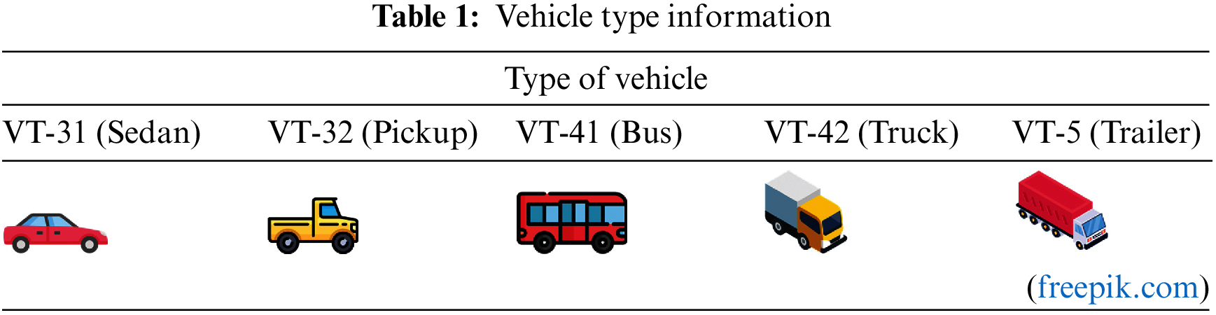
Table 2 shows this research’s feature information. The target for prediction in this study is the traffic flow of sedan-type vehicles (VT-31). Here we have three types of holidays, namely Weekday, Weekend, and Cont_Holiday. Weekday is a holiday condition that occurs on a Weekday (Monday to Friday), Weekend is a holiday condition that occurs on Saturday or Sunday, while Cont_Holiday is a continuation of holidays that can occur before or after a Weekday or Weekend. The weather features are divided into numeric and categorical types. Wind speed and humidity are numeric since their values are numeric. The wind speed values are float numbers ranging from 0 to 15.95, and the humidity values are integer numbers going from 0 to 100. Meanwhile, other types of weather are categorical with a boolean value.

3  Proposed Method

Combining CNN and LSTM, a hybrid CNN-LSTM model is created to enhance traffic flow prediction better performance. The CNN-LSTM method for traffic flow prediction comprises a series of links between CNN and LSTM. This technique employs the CNN network’s convolutional and ReLU activation layers. CNN uses convolution to learn these complicated traffic flow characteristics, such as timestamped information and the previous day’s traffic flow value. Convolution can diminish the number of neuron parameters and increase the hybrid model’s depth.

The proposed combination CNN-LSTM method is a prediction approach that inputs 2-dimension heterogeneous time series data and outputs multistep time series data. Fig. 3 shows how the data is represented. The row section shows information based on time sequence with 1-h intervals, and the column section is a feature of the research data. We construct data represented as an image with a row size of 168 h (one week) and columns adjusted to the number of features used.

Figure 3: Data representation

The next step is to normalize the compiled data by applying Eq. (1) to transform the values from 0 to 1. Because each feature has a unique range of maximum and minimum values, the normalization procedure is performed separately for each feature. Here, xnorm is the value after the scaling process. X(r,c) is the value in feature c, row r. X(c)min and X(c)max represent the minimum and maximum value for feature c, respectively.

Xnorm=x(r,c)−x(c)minx(c)max−x(c)min(1)

After the data has been normalized, it is separated into training data (two years) and testing data (one year), as shown in Fig. 4. Windows slide data is one hour. W is input data represented as an image with dimensions r x c. The total input data is the result of calculating from the number of total row data (tr) minus the number of image row data (nr) plus the size of the windows slide (sw).

Figure 4: Training and testing data

Fig. 5 displays the process of applying 1-dimensional kernel size to the 2-dimension tensor input. There is only one direction of movement for the 1-dimensional kernel. Kernel size 1 means the size of the kernel is 1 x c. Here, c is the spatial length (feature’s condition), and r is the temporal length (time steps).

Figure 5: Applying 1-dimension kernel size to 2D input tensor [25]

Fig. 6 shows the detailed proposed method. Input data required for CNN-LSTM training are initially prepared. The model is divided into two parts, feature extraction, and time-series prediction. The data is subsequently transmitted to the CNN encoder for feature extraction purposes. The CNN encoder consists of two convolutional layers, each with 64 filters of kernel sizes 1 to 12 applying 1-dimensional convolution, followed by a max pooling layer. Convolutional neural networks (CNN) also implement stride moves. Stride refers to the number of pixels the filter shifts by in each step while performing the convolution operation on the input image [38]. Here we set the stride to 1, and the filter slides over the input image one pixel at a time. CNN works the convolution layer employs a pooling layer that merges the output of a neuron cluster from the preceding layer into a single neuron in the subsequent layer. The pooling layer aims to cut down on the data representation size and the number of parameters, which speeds up computation.

Figure 6: CNN-LSTM proposed method

The CNN encoder’s output is then flattened. Before the flattened CNN output data becomes the input for the LSTM, the repetition vector is executed 168 times based on the number of input neuron units in the LSTM. LSTM, a lower layer of CNN-LSTM, contains time information regarding the crucial feature of power demand retrieved by CNN. LSTM offers a solution by keeping long-term memory through the consolidation of memory units that can update the previous hidden state. This function simplifies the comprehension of temporal links in a lengthy sequence.

The output values from the preceding layer of CNN are sent to the LSTM gate units. By performing multiplication operations, the three gate units determine the state of each memory cell. After passing through the LSTM layer, a dropout mechanism is used to avoid overfitting. Dropout works by randomly setting a fraction of the input units to zero during each training iteration. From this point forward, the LSTM TimeDistributed procedure is executed. The TimeDistributed LSTM layer applies the same set of LSTM cells to each time step of the input sequence, enabling the network to model the sequence’s temporal relationships over time. A hidden state at the output of the TimeDistributed LSTM layer represents each time step of the input sequence. In this part, the total input and output are 168 units. The TimeDistributed LSTM stage is repeated with 168 input units and one output unit. At this point, the CNN-LSTM model’s final prediction is represented by its output arrangement. The output value calculated by the output layer is compared with the ground truth of the data, and the corresponding error is treated. The loss function (mean square error) represents the difference between the actual and predicted values.

4  Experimental Result

In the experimental results section, several stages were carried out. Firstly, is to prepare input data. The input data is divided into three scenarios: experiment with feature vehicle type, weather, and holidays. Furthermore, CNN-LSTM’s prediction results are compared to other traffic flow prediction models, including LSTM, BILSTM, and LSTM-BILSTM. Mean Absolute Error (MAE), Mean Square Error (MSE), and Root Mean Square Error (RMSE) [39] are the evaluations used. The following section offers the results of several trials carried out as follows: procedure of fine-tuning parameters is described in Section 4.1. The experimental findings using the input vehicle type are presented in Section 4.2. Holidays are the experimental results presented in Section 4.3. In Section 4.4, the experimental results with Weather input are presented. Section 4.5 displays the experimental outcomes with input from all features.

4.1 CNN-LSTM Hyperparameter Tunning

In this study, we conducted experiments to tune several parameters: the number of convolution layers, optimizer, learning rate, kernel size, dropout, filters, and batch size. The details hyperparameter used in this research can be seen in Table 3. By systematically adjusting these parameters and analyzing the resulting performance metrics, we identified the optimal combination for our particular task. Overall, our experiments provided valuable insights into the effects of these parameters on our model’s performance and enabled us to achieve the best possible results. We tested our model with Epoch values of 50, 100, 150, and 200 to find the best number of training epochs. For the optimizer, we tested SGD, RMSprop, and Adam to find the best optimization algorithm for our model. We experimented with Batch-Size values of 20, 25, 30, 50, and 100 to find the optimal number of training samples per batch. To prevent overfitting, we experimented with different values of Dropout, including 10%, 20%, 30%, and 40%. We also varied the learning rate, testing values of 0.1, 0.01, 0.001, and 0.0001 to find our model’s optimal rate of change. We utilized Mean Squared Error (MSE) as our loss function and experimented with different Pooling sizes of 2 and 4 to improve the accuracy of our model. Additionally, we varied the Kernel size from 1 to 12 and tested different values for the number of Filters, including 16, 32, 64, and 128. Overall, our experiments with these hyperparameters allowed us to identify our deep learning model’s best combination of values, improving its accuracy and performance.

According to the findings of the tests, the optimal values for the parameters are as follows: epoch 100, optimizer Adam, batch size 100, dropout 20%, pool size two, and the number of filters 64. In a CNN, a kernel is a small matrix of learnable parameters convolved with the input data to produce a feature map. The kernel systematically slides over the input data, extracting local patterns and features from the input. The size of the kernel is usually smaller than the input data, typically ranging from 1 × 1 to 12 × 12, and it is the same for all the input channels. On the other hand, a filter in CNN refers to a collection of kernels that are convolved with the input data to produce multiple feature maps. Each filter learns a different set of features from the input data, and the number of filters used in each layer determines the depth of the layer. For example, a layer with 16 filters will produce 16 feature maps as output, each generated by convolving the input data with a different kernel. Therefore, while a kernel is a small matrix that extracts local features from the input data, a filter is a collection of kernels that learns features from the input data and produces multiple feature maps as output. In this study, the size of the kernel varies from 1 to 12. We used standard convolution kernel adoption from [25]. Each kernel size impacts a different performance result in each experiment that is carried out.

Fig. 7 depicts the trained network topology of the proposed model, CNN-LSTM, which has 3,759,089 configurable parameters and receives 168 x number of feature matrices as input. Following convolutional neural networks layer feature extraction and LSTM layer time series prediction, the output matrix size is 168 × 1 vector. LSTM is an essential part of the CNN-LSTM framework that produces the traffic flow vector features based on the given traffic historical data.

Figure 7: CNN-LSTM parameter values

4.2 Vehicle Type Feature

The experiment shows a consistent result pattern in the MAE, MSE, and RMSE calculations. In particular, when the MAE value increases, there is an increase in the MSE and RMSE values, and if there is a decrease in the MAE performance, the prediction performance of MSE and RMSE also decreases. Before the experiment, each feature data is normalized to anticipate outlier values. Furthermore, in this section, performance improvement findings are presented based on the evaluation of the MAE matrix. A negative performance value indicates a decrease in predicted performance, while a positive value indicates an increase in predicted performance. The performance calculation is shown in Eq. (2), where Imp represents the percentage increase, Ov is the original value, and Nv is the new value.

Imp=Ov−NvOv * 100(2)

Table 4 shows the experimental results with only one type of traffic flow input feature from a sedan vehicle type (VT-31). The results of this prediction performance serve as a baseline for other experiments. This section uses the vehicle type input feature to conduct investigations. There are five types of vehicles, sedan, pickup, bus, truck, and trailer. Tests were carried out on four prediction models, LSTM, BILSTM, LSTM-BILSTM, and CNN-LSTM.

Table 5 displays the experimental outcomes utilizing the vehicle-type feature (sedan, pickup, bus, truck, and trailer). From experiments with variations in kernel size 1 to 12, the best performance is obtained when the kernel size is 2. Based on the MAE evaluation matrix, the prediction performance of the BILSTM and CNN-LSTM models increased by 7.40% and 23.7%, respectively. While the LSTM and LSTM-BILSTM models did not produce favorable findings, a drop of −6.89% and −6.96% was observed.

4.3 Holidays Feature

The following experiment is to determine the feature holiday’s impact on increasing prediction performance. There are three types of holiday features, Weekday, Weekend, and continuous holidays. Weekday is travel information that occurs from Monday to Friday. The Weekend is a vehicle trip that happens on Saturday or Sunday. Meanwhile, continuous holidays are vehicle trips before or after Weekends or Weekdays. Table 6 shows prediction performance results with holiday input with kernel size 6. The LSTM, BILSTM, and LSTM-BILSTM models did not give good results from the experimental results. There was a decrease in each model of −3.76%, −0.20%, and −7.95%. Meanwhile, in the CNN-LSTM model, there was an increase in performance of 14.02%. This result is not greater than the performance results with the input of the vehicle type feature.

4.4 Weather Feature

The following experiment will use weather data as input. Table 7 shows the model performance with weather feature input. There are two sorts of weather characteristics: numerical weather and categorical weather. Numerical weather pertains to wind speed and humidity, while categorical weather encompasses eight meteorological conditions: clear, cloud, drizzle, fog, haze, mist, rain, and thunderstorms. A kernel size of 6 yields the best performance prediction results based on weather inputs. In this experiment, LSTM performance decreased by −9.25%, while BILSTM performance decreased by −7.32%. While the performance of the other two models grew, LSTM-BILSTM 8.45% and CNN-LSTM 25.85%.

4.5 All Features

The last experiment was carried out with the input of all existing features. The input size is represented as an image measuring 168 × 18. Table 8 shows model performance with all features input. The testing findings demonstrate more outstanding performance than the input case with the holiday feature. The best performance condition occurs when the kernel size is 2. The prediction performance of the −10.84% LSTM and −9.12% BILSTM models decreased. In contrast, the LSTM-BILSTM and CNN-LSTM models showed an increase of 1.45% and 21.63%, respectively.

According to Fig. 8, the difference between the actual and forecasted values is relatively similar, confirming that the forecasting model utilized in this study is both possible and successful. However, the data prediction in the prediction outcomes of 65 to 70 timesteps does not perform satisfactorily. Traffic flow prediction models rely heavily on historical data to make predictions and have limitations regarding the scope and complexity of the traffic patterns they can predict.

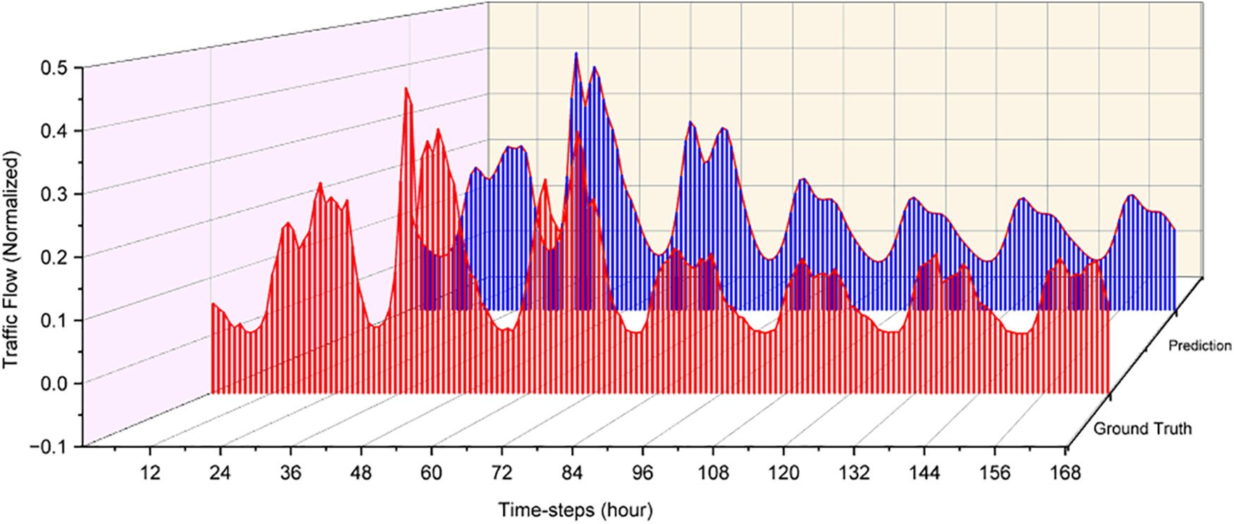
Figure 8: CNN-LSTM traffic flow model prediction with weather feature

5  Conclusion

This study provides a CNN-LSTM hybrid model for heterogeneous spatiotemporal correlation in traffic flow. Using a CNN, the proposed approach extracts spatial information from diverse spatiotemporal data, and the LSTM network extracts temporal features based on historical time-series traffic flow data. Both models combine the ability to find correlations between temporal and spatial data to generate predictions for traffic flow. Based on experimental results, the factors that most influence the increase in prediction performance are Weather (25.85%), Traffic Flow (23.70%), and Holiday (14.02%). In conclusion, the experimental results demonstrate that the proposed model to construct a spatiotemporal feature extraction method proved that it could improve prediction performance.

6  Discussion

Based on the experiment’s result, combining all the features does not guarantee the best performance. The basic concept behind convolution is identifying visually significant patterns in an image, such as a jigsaw puzzle, where the pieces’ arrangement determines the image’s meaning. Thus, the organization of spatiotemporal data has a significant impact on the information captured. There are endless possibilities for feature combinations, and future research will explore this area further.

Furthermore, per data-centric principles, the research will prioritize improving data quality during pre-processing. The spatiotemporal data will be obtained from both directions of the freeway and the neighboring freeway to gain a more comprehensive understanding of traffic flow. Moreover, alternative spatiotemporal correlation models will be investigated, and the developed model will be evaluated for traffic flow prediction in future studies.

Acknowledgement: The authors wish to extend their most profound appreciation to the anonymous referees for their informative and constructive feedback. This research was supported by Asia University and Universitas Muhammadiyah Yogyakarta, Indonesia.

Funding Statement: This Research was supported by Universitas Muhammadiyah Yogyakarta, Indonesia and Asia University, Taiwan. The author received no specific funding for this study.

Author Contributions: The authors confirm contribution to the paper as follows: study conception and design: Wang, Susanto; data collection: Wang; data processing: Wang, Susanto; analysis and interpretation of results: Susanto, draft manuscript preparation: Wang, Susanto. All authors reviewed the results and approved the final version of the manuscript.

Availibility of Data and Materials: Raw data material can be accessed in https://tisvcloud.freeway.gov.tw/history/TDCS/M06A/. Data sharing is not applicable to this article.

Conflicts of Interest: The authors declare that they have no conflicts of interest to report regarding the present study.

References

1. J. Zhang, F. Y. Wang, K. Wang, W. H. Lin, X. Xu et al., “Data-driven intelligent transportation systems: A survey,” IEEE Transactions on Intelligent Transportation Systems, vol. 12, no. 4, pp. 1624–1639, 2011. [Google Scholar]

2. W. Zhang, Y. Yu, Y. Qi, F. Shu and Y. Wang, “Short-term traffic flow prediction based on spatio-temporal analysis and CNN deep learning,” Transportmetrica A: Transport Science, vol. 15, no. 2, pp. 1688–1711, 2019. [Google Scholar]

3. X. Xu, Z. Fang, J. Zhang, Q. He, D. Yu et al., “Edge content caching with deep spatiotemporal residual network for IoV in smart city,” ACM Transactions on Sensor Networks, vol. 17, no. 3, pp. 1–33, 2021. [Google Scholar]

4. H. Wang, L. Liu, S. Dong, Z. Qian and H. Wei, “A novel work zone short-term vehicle-type specific traffic speed prediction model through the hybrid EMD–ARIMA framework,” Transportmetrica B: Transport Dynamics, vol. 4, no. 3, pp. 159–186, 2016. [Google Scholar]

5. M. Van Der Voort, M. Dougherty and S. Watson, “Combining kohonen maps with arima time series models to forecast traffic flow,” Transportation Research Part C: Emerging Technologies, vol. 4, no. 5, pp. 307–318, 1996. [Google Scholar]

6. S. Lee and D. B. Fambro, “Application of subset autoregressive integrated moving average model for short-term freeway traffic volume forecasting,” Transportation Research Record, vol. 1678, no. 1, pp. 179–188, 1999. [Google Scholar]

7. S. V. Kumar and L. Vanajakshi, “Short-term traffic flow prediction using seasonal ARIMA model with limited input data,” European Transport Research Review, vol. 7, no. 3, pp. 1–9, 2015. [Google Scholar]

8. B. M. Williams and L. A. Hoel, “Modeling and forecasting vehicular traffic flow as a seasonal ARIMA process: Theoretical basis and empirical results,” Journal of Transportation Engineering, vol. 129, no. 6, pp. 664–672, 2003. [Google Scholar]

9. M. M. Hamed, H. R. Al-Masaeid and Z. M. B. Said, “Short-term prediction of traffic volume in urban arterials,” Journal of Transportation Engineering, vol. 121, no. 3, pp. 249–254, 1995. [Google Scholar]

10. J. Guo, W. Huang and B. M. Williams, “Adaptive Kalman filter approach for stochastic short-term traffic flow rate prediction and uncertainty quantification,” Transportation Research Part C: Emerging Technologies, vol. 43, no. 2, pp. 50–64, 2014. [Google Scholar]

11. I. Okutani and Y. J. Stephanedes, “Dynamic prediction of traffic volume through Kalman filtering theory,” Transportation Research Part B: Methodological, vol. 18, no. 1, pp. 1–11, 1984. [Google Scholar]

12. Y. Xie, Y. Zhang and Z. Ye, “Short-term traffic volume forecasting using Kalman filter with discrete wavelet decomposition,” Computer-Aided Civil and Infrastructure Engineering, vol. 22, no. 5, pp. 326–334, 2007. [Google Scholar]

13. T. Zhou, D. Jiang, Z. Lin, G. Han, X. Xu et al., “Hybrid dual Kalman filtering model for short-term traffic flow forecasting,” IET Intelligent Transport Systems, vol. 13, no. 6, pp. 1023–1032, 2019. [Google Scholar]

14. C. Dong, S. H. Richards, Q. Yang and C. Shao, “Combining the statistical model and heuristic model to predict flow rate,” Journal of Transportation Engineering, vol. 140, no. 7, pp. 04014023, 2014. [Google Scholar]

15. E. I. Vlahogianni, J. C. Golias and M. G. Karlaftis, “Short-term traffic forecasting: Overview of objectives and methods,” Transport Reviews, vol. 24, no. 5, pp. 533–557, 2004. [Google Scholar]

16. Y. Kara, M. A. Boyacioglu and Ö. K. Baykan, “Predicting direction of stock price index movement using artificial neural networks and support vector machines: The sample of the Istanbul stock exchange,” Expert Systems with Applications, vol. 38, no. 5, pp. 5311–5319, 2011. [Google Scholar]

17. J. Wang and J. Wang, “Forecasting stock market indexes using principle component analysis and stochastic time effective neural networks,” Neurocomputing, vol. 156, pp. 68–78, 2015. [Google Scholar]

18. A. J. Smola and B. Schölkopf, “A tutorial on support vector regression,” Statistics and Computing, vol. 14, pp. 199–222, 2004. [Google Scholar]

19. E. Guresen, G. Kayakutlu and T. U. Daim, “Using artificial neural network models in stock market index prediction,” Expert Systems with Applications, vol. 38, no. 8, pp. 10389–10397, 2011. [Google Scholar]

20. S. Haykin and N. Network, “A comprehensive foundation,” Neural Networks, vol. 2, no. 2004, pp. 41, 2004. [Google Scholar]

21. D. Park and L. R. Rilett, “Forecasting freeway link travel times with a multilayer feedforward neural network,” Computer-Aided Civil and Infrastructure Engineering, vol. 14, no. 5, pp. 357–367, 1999. [Google Scholar]

22. J. Morton, T. A. Wheeler and M. J. Kochenderfer, “Analysis of recurrent neural networks for probabilistic modeling of driver behavior,” IEEE Transactions on Intelligent Transportation Systems, vol. 18, no. 5, pp. 1289–1298, 2016. [Google Scholar]

23. S. Gautam, A. Henry, M. Zuhair, M. Rashid, A. R. Javed et al., “A composite approach of intrusion detection systems: Hybrid RNN and correlation-based feature optimization,” Electronics, vol. 11, no. 21, pp. 3529, 2022. [Google Scholar]

24. K. T. Chui, B. B. Gupta and P. Vasant, “A genetic algorithm optimized RNN-LSTM model for remaining useful life prediction of turbofan engine,” Electronics, vol. 10, no. 3, pp. 285, 2021. [Google Scholar]

25. E. Hoseinzade and S. Haratizadeh, “CNNpred: CNN-based stock market prediction using a diverse set of variables,” Expert Systems with Applications, vol. 129, pp. 273–285, 2019. [Google Scholar]

26. D. Li, L. Deng, B. B. Gupta, H. Wang and C. Choi, “A novel CNN based security guaranteed image watermarking generation scenario for smart city applications,” Information Sciences, vol. 479, pp. 432–447, 2019. [Google Scholar]

27. J. Mackenzie, J. F. Roddick and R. Zito, “An evaluation of HTM and LSTM for short-term arterial traffic flow prediction,” IEEE Transactions on Intelligent Transportation Systems, vol. 20, no. 5, pp. 1847–1857, 2018. [Google Scholar]

28. A. Gumaei, M. Al-Rakhami, H. AlSalman, S. M. M. Rahman, A. Alamri et al., “DL-HAR: Deep learning-based human activity recognition framework for edge computing,” Computers, Materials & Continua, vol. 65, no. 2, pp. 1033–1057, 2020. [Google Scholar]

29. P. Zhang, C. Wang, C. Jiang and Z. Han, “Deep reinforcement learning assisted federated learning algorithm for data management of IIoT,” IEEE Transactions on Industrial Informatics, vol. 17, no. 12, pp. 8475–8484, 2021. [Google Scholar]

30. B. Mao, F. Tang, Y. Kawamoto and N. Kato, “AI models for green communications towards 6G,” IEEE Communications Surveys & Tutorials, vol. 24, no. 1, pp. 210–247, 2021. [Google Scholar]

31. Z. M. Fadlullah, F. Tang, B. Mao, N. Kato, O. Akashi et al., “State-of-the-art deep learning: Evolving machine intelligence toward tomorrow’s intelligent network traffic control systems,” IEEE Communications Surveys & Tutorials, vol. 19, no. 4, pp. 2432–2455, 2017. [Google Scholar]

32. P. Zhang, Y. Wang, N. Kumar, C. Jiang and G. Shi, “A security-and privacy-preserving approach based on data disturbance for collaborative edge computing in social IoT systems,” IEEE Transactions on Computational Social Systems, vol. 9, no. 1, pp. 97–108, 2021. [Google Scholar]

33. X. Ma, Z. Dai, Z. He, J. Ma, Y. Wang et al., “Learning traffic as images: A deep convolutional neural network for large-scale transportation network speed prediction,” Sensors, vol. 17, no. 4, pp. 818, 2017. [Google Scholar] [PubMed]

34. Z. Yang, J. Yang, K. Rice, J. L. Hung and X. Du, “Using convolutional neural network to recognize learning images for early warning of at-risk students,” IEEE Transactions on Learning Technologies, vol. 13, no. 3, pp. 617–630, 2020. [Google Scholar]

35. J. D. Wang and M. C. Hwang, “A novel approach to extract significant patterns of travel time intervals of vehicles from freeway gantry timestamp sequences,” Applied Sciences, vol. 7, no. 9, pp. 878, 2017. [Google Scholar]

36. J. D. Wang, “Extracting significant pattern histories from timestamped texts using MapReduce,” The Journal of Supercomputing, vol. 72, pp. 3236–3260, 2016. [Google Scholar]

37. W. Ching-Tu, “Method for extracting maximal repeat patterns and computing frequency distribution tables,” ed: Google Patents, 2019. [Online]. Available: https://patents.google.com/patent/US20170255634A1/ [Google Scholar]

38. S. Lee, Y. Ahn and H. Y. Kim, “Predicting concrete compressive strength using deep convolutional neural network based on image characteristics,” Computers, Materials & Continua, vol. 65, no. 1, pp. 1–17, 2020. [Google Scholar]

39. L. Lv, Z. Wu, L. Zhang, B. B. Gupta and Z. Tian, “An Edge-AI based forecasting approach for improving smart microgrid efficiency,” IEEE Transactions on Industrial Informatics, vol. 18, no. 11, pp. 7946–7954, 2022. [Google Scholar]