Reliability Analysis of Correlated Competitive and Dependent Components Considering Random Isolation Times

1  Introduction

With the advancement of communication technology, the development of the IoT has reached a new stage [1,2]. In the IoT environment, all objects in our daily lives are part of the Internet, due to their communication and computing capabilities (including microcontrollers and digital communication transceivers). The IoT extends the concept of the Internet and makes it more pervasive, allowing different devices to interact while keeping their data secure (e.g., medical sensors, surveillance cameras, household appliances, etc.) [3,4]. Body Sensor Network technology [5] is one of the most critical technologies in modern IoT-based healthcare systems. The BSN system is often used to detect some physiological characteristics of people [6,7], and it is widely used in medical care, military, fitness, firefighting, and sports fields.

A BSN system consists of the following three parts: biomedical sensors [8], relay nodes, and sink nodes. In this work, sink nodes are considered to be completely reliable. Other BSN components will only suffer from local failure (LFs) and propagation failure (PFs). LF will only lead to the failure of the component itself without affecting other components in the system, while PF will not only cause the failure of the component itself but also affect other components in the system [9,10]. Note that the PFs used in this article are propagation failure with global effects (PFGEs), if one PF occurs, the entire system will fail. In the BSN system, the energy of the biosensor comes from the batteries [11,12]. If the transmission distance is long, the perceived information can be transmitted to the target through relay communication [13–15] to achieve the purpose of energy saving.

When the relay node fails, the remaining time during which a sensor node can communicate directly with the receiving device is determined by its remaining battery energy. In other words, the timing of the isolation effect is random. When the isolation effect occurs, it may have a dual effect: on the one hand, the performance of the system will be degraded, because when the biosensor is isolated, the receiving device will not receive the information it perceives on time; on the other hand, because the biosensor is isolated at this point, the PFs from this biosensor can be prevented from damaging other components in the system (such as jamming attacks [16,17], overheating, and short-circuits [18]). However, when the PF of the biosensor in the system occurs before the relay failure or the biosensor PF occurs after a relay failure but the biosensor has enough power to transmit data directly to the receiving node, there will be a propagation effect and make the whole system fail. Therefore, a time-domain competition exists between the PF isolation effect and the PF propagation effect. When the isolation effect occurs first, the system will not fail, and the BSN system will continue to work with reduced performance. Otherwise, if the propagation effect prevails, the system will fail. So, there are many existing papers on competition failure. Unfortunately, there are few papers that consider random isolation time (RIT). More details are given in Section 2.

The rest of this paper is structured as follows: Section 2 is the related work. Section 3 introduces the new combinatorial analysis algorithm. Section 4 takes the BSN system as an example to analyze the proposed algorithm. The numerical analysis is carried out in Section 5. Section 6 summarizes the work and discusses future directions.

2  Related Work

Solving competition failure problems has become a deep research field. There are different approaches to reliability analysis for different types of functional-dependent systems. The simulation method is highly applicable to all kinds of systems in the modeling of system behavior, but the results calculated by the simulation method are usually not accurate enough and can only provide rough results. If the calculation accuracy needs to be improved, the time cost will increase, so it is not suitable for accurate calculation of the reliability of large-scale systems [19,20]. Markov method can flexibly simulate all kinds of dynamic behavior and is common to solve the problem of dynamic system reliability analysis method, but the method of Markov has the state space explosion problem [21,22].

This combination method has the advantages of high precision and high efficiency and is widely used in the reliability analysis of systems with competing faults. The combinatorial algorithm is used to solve the reliability analysis problem of single-stage [23] and multi-stage [24] systems in deterministic competitive faults. For probabilistic competitive faults [25], random fault propagation time [26] is considered. The failure propagation time [27] is considered from the multi-function dependency group and the cascading [28] behavior is considered in competitive failure.

In the case of relay failure, the study of random isolation time (RIT) and competition effect becomes very important in reliability analysis. However, as far as we know, few existing works consider or assume zero RIT when conducting reliability analyses. Although the literature [29] considered the effect of competing failures and random isolation times on system reliability, the approach in this work assumes that when transmitting data, the biosensors cannot use the same relay node, and is therefore not applicable to systems in which the same relay needs to be used for transmission.

In this paper, the failure of the competition combination method was improved compared with existing methods. This article considers the effects of competitive failure and random isolation time on system reliability and allow different biological sensors to use the same relay when transmitting data, solving the problem of data transmission among different biological sensors in the system that need to use the same relay. At the same time, the system element in this method can follow any failure time distribution. Please note that although this article is based on a discussion of BSN systems, the competitive failure behavior and the proposed method can be applied to other application systems, such as computer networks, smart homes, smart grids, etc.

3  Proposed Method

According to the total probability theorem and divide-and-conquer principle, the reliability of the BSN system with competitive effect can be decomposed into several independent simplified problems without competitive effect.

3.1 Establish Fault Tree(FT) Model and Separate PF

The FT model is used to express the system’s fault behavior by ignoring the components’ propagating failure behavior. In the BSN system, the BSN system failing is the top event, and the relay component failure and the dependent component failure is the basic event. The sensor communicates with the receiver through the relay; thus, there is a functional dependency between the sensor and the relay. The functional dependency (FDEP) behavior in the dynamic FT model can be modeled in Fig. 1.

R(t)=Pu(t)⋅CR(t)(1)

Figure 1: Functional dependency behavior in BSN

Pu(t) in Eq. (1) is the probability that PF does not occur in mission time (0,t], Pu(t)=∏∀i∈I[1−qiPF(t)], where the set I is the set of all experiencing PF components, while qiPF(t) is the probability of component i experiencing PF. According to its definition, the calculation process of CR(t) can be given by the following steps.

Note that the failure probability of component i should be replaced by the conditional failure probability of component i (denoted as qi(t)) when calculating the local failure probability of component i. Suppose that qil is denotes the probability of the local failure of a component, and while qip is the probability of the propagated failure of a component. When local and propagated failures are mutually exclusive, the conditional probability of component failure can be calculated using Eq. (2). When local and propagated failures are s-independent, the conditional probability of component failure can be computed using Eq. (3):

qi(t)=Pr(iLF|iPF¯)=Pr(iLF|iPF¯)Pr(iPF¯)=Pr(iLF)Pr(iPF¯)=qil(t)1−qip(t)(2)

qi(t)=Pr(iLF|iPF¯)=Pr(iLF)×Pr(iPF¯)Pr(iPF¯)=qil(t)(3)

3.2 Build Event Space according to Relay LF and Dependent Components PF

The next step is to construct an event space to consider all possible combinations of failure states for the relay component and dependent components. In the system under consideration, there exists one relay node T and n dependent nodes Di(i=1,2,…,n) generating 2n+1 disjoint events. Events E1,E2,E3,E4 denote the combination of LF and PF occurring and not occurring, respectively.

E1: The relay node works normally, and no PF occurs in the dependent components Di. In this case, no isolation effect or propagation effect occurs.

E2: The relay node works normally, and at least one dependent component has PF. At this time, the propagation effect will cause the system to fail.

E3: LF occurs in the relay node, and PF does not occur in any dependent components. In this case, isolation effects occur without propagation effects, and the corresponding dependent components are isolated.

E4: LF occurs in the relay node (TLF), and PF occurs in at least one dependent component (denoted as DiPF). When E4 occurs, TLF and DiPF occurs simultaneously, and the time domain competition leads to three disjoint competition events, denoted as CE1,CE2,CE3; that is, E4=CE1∪CE2∪CE3. CE1 indicates that PF occurs in at least one dependent component occurs PF before the LF of the relay node (DiPF→TLF), at which time a global propagation effect will occur, making the system fail. CE2 indicates that the dependent components have experienced PFs and all PFs occur after the LF of the relay node (TLF→DiPF), but the RIT of at least one dependent component is not less than the difference between the occurrence time of TLF and DiPF (DiIT¯), this means that the biosensor Di is isolated after the occurrence of DiPF (DiI). At this time, the system fails because of the propagation effects that occur. CE3 indicates that PF occurs in the dependent components and all PFs occur after the LF of the relay node, but the RIT of at least one dependent component is less than the difference in time of occurrence between TLF and DiPF (DiIT). This means that DiI occur before DiPF, in this case, the isolation effect will occur.

Table 1 provides the definition of (E1, E2, E3, E4). Here, TLF and TLF¯ indicate that LF occurrence and nonoccurrence for T; DiPF and DiPF¯ denote the occurrence and nonoccurrence of PF of Di, respectively.

In BSN system, SR is used to indicate system reliability. According to the event space (E1,E2,E3,CE1,CE2,CE3) as defined, CRBSN(t) can be calculated:

CRBSN(t)=Pr(SR∩E1)+Pr(SR∩E2)+Pr(SR∩E3)+Pr(SR∩CE1)+Pr(SR∩CE2)+Pr(SR∩CE3)(4)

Because the system will occur propagation effects at E2, CE1 and CE2, Pr(SR∩E2), Pr(SR∩CE1) and Pr(SR∩CE2) are equal to zero. Therefore, Eq. (4) can be simplified as follows:

CRBSN(t)=Pr(SR∩E1)+Pr(SR∩E3)+Pr(SR∩CE3)(5)

3.3 Address Propagation Effects and Isolation Effects

Pr(SR∩E1): In this case, according to the definition of E1, no propagation effect or isolation effect occurs. So, Pr(E1)=∑i=1n[1−qTL(t)][1−qDiPF(t)]. Depending on the conditional probabilities, Pr(SR∩E1) can be computed by Eq. (6):

Pr(SR∩E1)=∑i=1n[1−qTL(t)]⋅[1−qDiPF(t)]⋅Pr(SR|E1)(6)

where Pr(SR|E1) (reliability of BSN systems conditional on the occurrence of E1), according to Eq. (1) and simplified FT model. The FT is generated by removing T and the corresponding FDEP gate but keeping Di from the old FT.

Pr(SR∩E3): When E3 occurs, the LF of the relay node occurs, but there is no PF from Di(i=1,2,…,n). Based on isolation state of Di, E3 can be replaced by 2n disjoint events. Thus,

Pr(SR∩E3)=∑i=02n−1Pr(SR∩E3∩DiI)=∑i=02n−1Pr(E3∩DiI).Pr(SR|E3∩DiI)(7)

where Pr(E3∩DiI) is shown in Eq. (8), while Pr(SR|E3∩DiI) can be solved by generating a simplified FT model and using the binary decision diagram (BDD) method.

Pr(E3∩DiI)=Pr(TLF∩D1PF¯∩D2PF¯∩…∩DnPF¯∩DiI)=Pr(D1PF¯∩D2PF¯∩…∩DnPF¯)⋅Pr(TLF∩DiI)(8)

Pr(SR∩CE3): In this time, the isolation effect will occur. By the definition of CE3, it can be decomposed into 2n−1, namely (CE3,1,CE3,2,…,CE3,2n−1). Thus, the formula can be converted as follows:

Pr(SR∩CE3)=Pr{SR∩(CE3,1∪CE3,2∪…∪CE3,2n−1)}=∑j=12n−1Pr(SR|CE3,j)⋅Pr(CE3,j)(9)

3.4 Reliability of the Integrated BSN

By calculating Pr(SR∩E1), Pr(SR∩E3) and Pr(SR∩CE3) in the above steps, and then using Eq. (5) to obtain CRBSN(t). Moreover, by applying Eq. (1), the reliability of the final BSN can be further obtained.

4  Examples and Analysis

Fig. 2 gives a BSN system with five nodes. More specifically, biosensors B1, B2, H1 and H2 are used to monitor human blood pressure and heart rate, respectively. The relay node T transmits the data of the biosensors B1 and H1 to the receiving device; the receiving device will collect and process the data from all biosensors to assist the caregiver in taking action.

Figure 2: BSN model

When T experiences LF, B1 and H1 can increase their transmission power to communicate directly with the receiving device until the battery power of B1 and H1 is exhausted to the point that it can no longer support direct communication, at which time biosensors B1 and H1 will be isolated from the rest of the BSN system.

4.1 Establishing the FT Model and Separating PF

The modeling of the BSN system is shown in Fig. 3. The top event of this dynamic FT model is the BSN system fault, the basic event is the local fault of the relay node and biosensor nodes, and the FDEP gate simulates functional dependence behavior in the relay node and biosensor nodes. Applying Eq. (1), Pu(t) is the probability when no PF is generated; that is, Pu(t)=(1−qTPF). CR(t) represents the conditional probability of system failure without PF generation in independent components, which can be solved by Eq. (5).

Figure 3: FT of the BSN mode

4.2 Constructing the Event Space

According to Fig. 2, this BSN system has one relay node and two dependent nodes. The event space is built as defined in Section 3.2, as shown in Table 2. According to Eq. (5) and the event space definition provided in Table 2, Pr(SR∩E1), Pr(SR∩E3), and Pr(SR∩CE3) can be calculated from Section 4.3.

4.3 Calculating Pr(SR∩E1),Pr(SR∩E3) and Pr(SR∩CE3)

Pr(SR∩E1): In the event of E1, relay node T is reliable for the duration of the mission time, and neither biosensors B1 nor H1 will undergo PF.

Pr(E1)=Pr(TLF¯∩B1PF¯∩H1PF¯)=(1−qTL)⋅(1−qB1PF)⋅(1−qH1PF)(10)

Fig. 4a presents the simplified system FT model for evaluating Pr(SR∩E1), this simplified FT model can be obtained by removing T and FDEP from the original FT in Fig. 2, and its BDD model is shown in Fig. 4b. Because the simplified model has components that experience PF, it can be calculated using Eq. (1), Pr(SR∩E1)=Pu−E1(t)CRE1(t)Pu−E1=(1−qB2PF)⋅(1−qH2PF); CRE1(t) can be solved by the corresponding BDD model, as shown in Eq. (11).

CRE1=(1−qB1L⋅qB2L)⋅[(1−qH1L)+qH1L⋅(1−qH2L)](11)

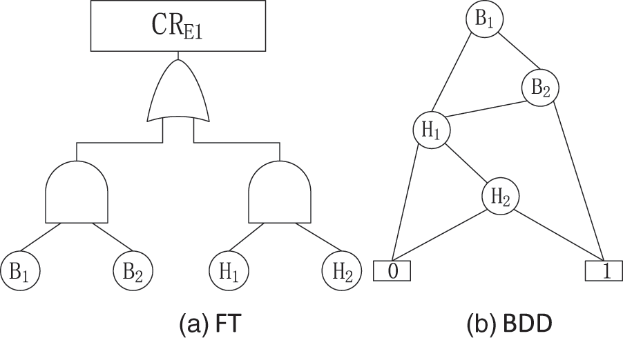
Figure 4: The FT and BDD of CRE1

Pr(SR∩E3): The LF of T occurs in the case of E3, but without PF from any Di. Depending on the isolation state of Di, E3 can be further decomposed into 2n complementary events: (B¯1,H¯1),(B1,H¯1),(B¯1,H1),(B1,H1). D0I indicate that neither B1 nor H1 is isolated by relay node T, and D3I indicate that both B1 and H1 are isolated by T. Pr(SR∩E3) is computed in Eq. (12).

Pr(SR∩E3)=∑i=03Pr(SR∩E3∩DiI)=∑i=03Pr(E3∩DiI)⋅Pr(SR|E3∩DiI)(12)

Pr(E3∩DiI) can be solved according to the definition and input parameters, Pr(E3∩D0I),

Pr(E3∩D1I), Pr(E3∩D2I) and Pr(E3∩D3I) as shown below:

Pr(E3∩D0I)=qTL⋅(1−qB1PF)⋅(1−qH1PF)⋅(1−qB1I)⋅(1−qH1I)(13)

Pr(E3∩D1I)=qTL⋅(1−qB1PF)⋅(1−qH1PF)⋅(1−qH1I)⋅qB1I(14)

Pr(E3∩D2I)=qTL⋅(1−qB1PF)⋅(1−qH1PF)⋅(1−qB1I)⋅qH1I(15)

Pr(E3∩D3I)=qTL⋅(1−qB1PF)⋅(1−qH1PF)⋅qB1I⋅qH1I(16)

Pr(SR|E3∩DiI) can be simplified through the removal of rules from the FT in Fig. 2 (relay nodes and related PFDG), which enables the simplified FT model to be generated for evaluation. For example, the simplified system model of Pr(SR|E3∩D1I) is shown in Fig. 5. The reduced FT in Fig. 5a is generated by removing the relay fault and FDEP gate from the FT in Fig. 2. Replacing the fault event “B1” with “1”, and then applying the Boolean reduction rules (1AND B2=B2).

Pr(SR|E3∩D1I)=(1−qB2L)⋅[(1−qH1L)+qH1L⋅(1−qH2L)](17)

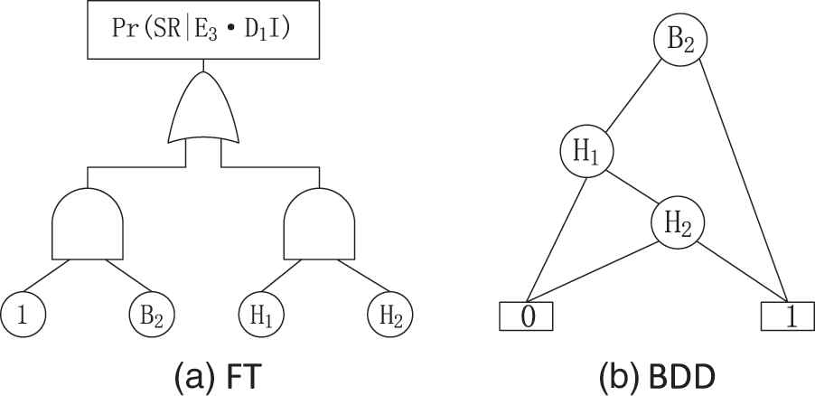
Figure 5: The FT and BDD of Pr(SR|E3⋅D1I)

Similarly, Pr(SR|E3∩D0I), Pr(SR|E3∩D2I) and Pr(SR|E3∩D3I) can be calculated.

Pr(SR|E3∩D0I)=(1−qB1L⋅qB2L)⋅[(1−qH1L)+qH1L⋅(1−qH2L)](18)

Pr(SR|E3∩D2I)=qB1L⋅qH2L+(1−qB1L)⋅qB2L⋅qH2L(19)

Pr(SR|E3∩D3I)=qB2L⋅qH2L(20)

Pr(SR∩CE3): In the case of CE3, the isolation effect will occur. According to Table 2, the event E3 consists of three events: namely, E3=CE3,1∪CE3,2∪CE3,3. The solution of Pr(SR∩CE3) can be converted to finding Pr(SR∩CE3,j)(j=1,2,3). Thus,

Pr(CE3,1)=Pr[(TLF→B1PF)∩B1IT∩H1PF¯](21)

Pr(CE3,2)=Pr[(TLF→H1PF)∩H1IT∩B1PF¯](22)

Pr(CE3,3)=Pr{[(TLF→B1PF)∩B1IT∩H1PF¯]∩[(TLF→H1PF)∩H1IT∩B1PF¯]}(23)

Pr(SR|CE3,j) can be calculated by generating FT.

Pr(SR|CE3,1)=(1−qB2L)⋅[(1−qH1L)+qH1L⋅(1−qH2L)](24)

Pr(SR|CE3,2)=qB1L⋅qH2L+(1−qB1L)⋅qB2L⋅qH2L(25)

Pr(SR|CE3,3)=qB2L⋅qH2L(26)

4.4 Integrated System Reliability

By calculating Pr(SR∩E1), Pr(SR∩E3) and Pr(SR∩CE3) in the above steps, CRBSN(t) can be obtained using Eq. (5). Moreover, by applying Eq. (1), the reliability of the final BSN can be further obtained.

5  Numerical Analysis

The combined method employed herein is suitable for any failure time distributions of biosensors. The numerical analysis of system reliability in this paper is based on Weibull distribution in Weibull distribution. The probability density function for a random variable c conforming to a Weibull distribution is given below; where, (α,k) denotes the (shape, scale) parameters, respectively.

fc(t)=kαkt(k−1)e−(αt)k(27)

The expectation or average of c is as follows:

E[c]=1α∫0∞e−tt1kdt(28)

Let (αiLF,kiLF),(αiPF,kiPF),(αiIT,kiIT) respectively represent the parameters of variable the time-to-LF, the time-to-PF, and RIT of component i under Weibull distribution, as shown in Table 3. Their expected values are expressed by the average time to LF (ATL), the average time to PF (ATP), and the average time to IT (ATI), respectively, which can be calculated by Eq. (28). Note that the combined method presented in this paper is a system-level’s analytical method and the component-level’s parameters are assumed from the biosensor’s industrial data.

5.1 Impact of RIT on System Reliability

This section studies the effect of RIT of dependent components B1 and H1. Because LF and PF parameters of a component have different influences on system reliability when they are s-independent and disjoint, Eqs. (2) and (3) can be used to calculate. This paper analyzes the influence when LF and PF are s-independent.

For ease of calculation, B1 and H1 have the same RIT parameters. The BSN system’s reliability is analyzed by the combination method detailed in Section 3. For the biosensors B1 and H1 with Weibull RIT, the shape parameter kiIT = 1. The scale parameter αIT (per h) and ATI of B1 and H1 are shown in Table 4. Table 4 summarizes the analysis results of the system reliability of LF and PF at different mission times.

According to the data given in Table 4, the reliability of the system decreases with an increase in task duration. Because the probability of failure of a biosensor in the system increases with increasing mission time. Obviously, the reliability of the system will continue to decrease under these circumstances.

In all cases, the system will exhibit different levels of reliability with different values of αIT. As can be seen intuitively, the ATI of dependent components increases with the decrease of αIT, the reliability of the BSN system presents an increasing, non-monotonic, and decreasing phenomenon at 48, 96 and 144 h.

In more detail, with the increase of αIT, the isolation probability of biosensors B1 and H1 also increases. In short, system reliability will be increased (positive effect) or decreased (negative effect) due to the interaction between the occurrence probability of the event SR∩E3∩DiI. Table 5 summarizes the influences of different dominant effects on system reliability in different time regions. When the propagation and isolation effects of B1 and H1 occur simultaneously, another dual effect will occur: first, the relay fault will isolate B1 and H1, thus preventing the PF of nodes B1 and H1 affecting other components in the system; second, the isolation effect makes the dependent nodes B1 and H1 unusable or inaccessible, which degrades the system’s performance. Moreover, on the one hand, the negative effect will reduce the reliability of the system, while on the other hand, the improvement effect will increase the reliability of the system. The change in BSN system reliability during mission time is caused by the combination of improvement and negative effects. With increasing αIT, the system reliability decreases under the action of the negative effect at 48 h; at 96 h, the system reliability initially decreases due to the negative effect, while the improvement effect increases the system reliability as αIT increases.

5.2 PF Impact on System Reliability

As summarized in Table 6, when the value of αiPF of dependent components increase to 1.7e-3, 2e-3 and 2.2e-3, using the parameters in Table 2, and the isolation time is (αIT=8.33e−4,k=1).

As can be seen from the results in Table 6, when the αiPF increase (ATP decreases at this time), the reliability of the whole system will decrease (that is, the unreliability of the system will increase). Because as αiPF increases, the probability of PF in the system increases, which obviously increases the system’s unreliability. Moreover, the passage of time has a more significant impact on system reliability. As the mission time increases, the influence of αiPF on system’s reliability ranges from 1.23% (calculated as (0.969440–0.957646)/0.957646) for 48 h to 9.01% (calculated as (0.763712–0.700598)/0.700598) for 144 h. This can be explained by the low likelihood that B1 and H1 will be isolated at the beginning of the task because the relays are so reliable. Therefore, the PF of B1 and H1 has a great influence on system reliability, in other words, with the increase of PF probability in B1 and H1, the reliability of the BSN system decreases. As the task time progresses, with the relay node deteriorating, B1 and H1 are more likely to be isolated. Although the propagation effects of B1 and H1 are weakened by isolation effects, the reliability of the system is reduced because of the aging of other components in the system.

5.3 Impact of LF on System Reliability

Table 7 summarizes when the value of αiLF of relay node increase to 1.5e-2, 2.7e-2 and 5e-2, using the parameters in Table 2, the isolation time is (αIT=8.33e−4,k=1).

The results in Table 7 show that the reliability of the entire system will change to a certain extent when the αiLF increases (ATL decreases at this time). In more detail, the system reliability first decreases and then increases at t = 48 h. Moreover, at t = 96 and t = 144 h, the system reliability exhibits an upward trend. This is because, at the beginning of the task when αRLF is relatively small, the relay still has high reliability, meaning that the probability of isolation effect is low; this means that the PF in the dependent node cannot be isolated in time, which results in a reduction in system reliability. However, with the increase of αRLF, the probability of relay failure will also increase, which in turn increases the probability of isolation effect in the BSN system and improves the system reliability. For example, with the passage of task time, when t = 96 and t = 144 h, the probability of component failure in the system increases, and the isolation effect also increases; thus, the system reliability tends to increase overall.

5.4 Evaluation

As far as we know, there are few algorithms for random isolation time. Table 8 lists the combinatorial algorithms for calculating system reliability with three competing failures. C1 considers the impact of competitive failure on system reliability; C2 is considering the influence of fault propagation time on system reliability, the propagation time is (αPT,kPT)=(1e−2/h, 1.0); Both C3 and the proposed algorithm consider the influence of RIT on system reliability, C3 assumes that only the dependent node H1 is affected by the relay node, and the isolation time is (αIT,kIT)=(4.17e−2/h, 2.0).

C1 only focuses on the evaluation of system reliability in the case of competitive failure. C2 studies the influence of fault propagation time on system reliability on the basis of C1. Neither C1 nor C2 takes into account the impact of random isolation time on system reliability, while C3 takes into account the impact of RIT on system reliability, but it has strong limitations and is only applicable to the case of one dependent node. The algorithm proposed in this paper solves the calculation problem of system reliability in the case of any dependent nodes.

Note that when the number of dependent nodes is reduced to one, the method presented in this article is the same as for C3. Assume that only H1 depends on the relay node and the LF and PF of the same node are s-independent. Using the parameters in Table 3, (αIT,kIT)=(4.17e−2/h,2.0), the reliability of the system (t = 24 h, 48 h, 72 h) is (0.9711, 0.9050, 0.8165), which is consistent with the results obtained by the method in this paper.

6  Conclusions

In IoT systems, the energy of the biosensor comes from the batteries. Because of the existence of FDEPs, there are propagation effects and isolation effects compete with each other in time and have to consider the RIT problem However, to the best of our knowledge, existing working assumptions assume that isolation time is zero or that the relay node supports only one dependent node. In this paper, a combination method is proposed for computational reliability analysis to analyze RIT behavior. Although the Weibull distribution is used in this case, the method can be used for any type of failure time distribution. This method can decompose complex problems and then calculate them by traditional methods. Note that although the BSN system is used in this case study, the method can be used for any wireless communication system. Notably, this method assumes that the biosensor can only use one relay for data transmission. In our future work, we intend to allow multiples of the same sensor to use different relay nodes for data transmission, solving the problem of correlation between multiple groups of related FDEP.

Acknowledgement: The authors also gratefully acknowledge the helpful comments and suggestions of the reviewers, which have improved the presentation.

Funding Statement: This work was supported by the National Natural Science Foundation of China (NSFC) (Grant No. 62172058) and the Hunan Provincial Natural Science Foundation of China (Grant Nos. 2022JJ10052, 2022JJ30624).

Author Contributions: The authors confirm contribution to the paper as follows: study conception and design: Shuo Cai and Tingyu Luo; data collection: Tingyu Luo and Fei Yu; analysis and interpretation of results: Shuo Cai and Pradip Kumar Sharma; draft manuscript preparation: Weizheng Wang. All authors reviewed the results and approved the final version of the manuscript.

Availability of Data and Materials: The data used for the findings of this study are available within this article.

Conflicts of Interest: The authors declare that they have no conflicts of interest to report regarding the present study.

References

1. K. R. S. Reddy, C. Satwika, G. Jaffino and M. K. Singh, “Monitoring of infrastructure and development for smart cities supported by IoT method,” in Proc. of Int. Conf. in Mechanical and Energy Technology, Singapore, Springer, pp. 21–28, 2023. [Google Scholar]

2. S. Ali and S. Parveen, “IoT-based smart healthcare monitoring system: A prototype approach,” Ph.D. Dissertation, Jamia Hamdard University, India, 2023. [Google Scholar]

3. J. Wang, W. Chen, L. Wang, Y. Ren and R. S. Sherratt, “Blockchain-based data storage mechanism for industrial Internet of Things,” Intelligent Automation and Soft Computing, vol. 26, no. 5, pp. 1157–1172, 2020. [Google Scholar]

4. A. Vangala, A. K. Das, Y. H. Park and S. S. Jamal, “Blockchain-based robust data security scheme in IoT-enabled smart home,” Computers, Materials & Continua, vol. 72, no. 2, pp. 3549–3570, 2022. [Google Scholar]

5. N. I. Hossain and S. Tabassum, “An IoT-enabled electronic textile-based flexible body sensor network for real-time health monitoring in assisted living during pandemic,” in ISQED, Santa Clara, CA, USA, pp. 1–5, 2022. [Google Scholar]

6. I. Borz, T. Palade, E. Puschita and A. Pastrav, “Wireless sensor networks for healthcare monitoring,” in Int.Conf. on Advancements of Medicine and Health Care Through Technology, Cham, Springer, pp. 232–239, 2020. [Google Scholar]

7. A. M. Abbas, “Body sensor networks for healthcare: Advancements and solutions,” Ph.D. Dissertation, Aligarh Muslim University, India, 2022. [Google Scholar]

8. J. Wang, Y. Gao, C. Zhou, S. Sherratt and L. Wang, “Optimal coverage multi-path scheduling scheme with multiple mobile sinks for WSNs,” Computers, Materials & Continua, vol. 62, no. 2, pp. 695–711, 2020. [Google Scholar]

9. L. Xing and G. Levitin, “Combinatorial analysis of systems with competing failures subject to failure isolation and propagation effects,” Reliability Engineering & System Safety, vol. 95, no. 11, pp. 1210–1215, 2010. [Google Scholar]

10. G. Levitin and L. Xing, “Reliability and performance of multi-state systems with propagated failures having selective effect,” Reliability Engineering & System Safety, vol. 95, no. 6, pp. 655–661, 2010. [Google Scholar]

11. J. Liang, Q. Sun, X. Wang, J. Xu, H. Wang et al., “Coverage control for underwater sensor networks based on residual energy probability,” Computers, Materials & Continua, vol. 73, no. 3, pp. 5459–5471, 2022. [Google Scholar]

12. J. Wang, Y. Gao, X. Yin, L. Feng and J. K. Hye, “An enhanced PEGASIS algorithm with mobile sink support for wireless sensor networks,” Wireless Communications and Mobile Computing, vol. 2018, no. 1, pp. 5459–5471, 2018. [Google Scholar]

13. S. Yousaf, N. Javaid, Z. A. Khan, Q. Umar, I. Muhammad et al., “Incremental relay based cooperative communication in wireless body area networks,” Procedia Computer Science, vol. 52, no. 1, pp. 552–562, 2015. [Google Scholar]

14. D. K. Rout and S. Das, “Hybrid relaying for sensor to external communication in multi relay body area networks,” in IEEE. Int. Conf. on SPICES, Kozhikode, India, pp. 1–5, 2015. [Google Scholar]

15. A. Dasgupta, M. M. Mennemanteuil, M. Buret, C. Nicolas, A. Bouhelier et al., “Optical wireless link between a nanoscale antenna and a transducing rectenna,” Nature Communications, vol. 9, no. 1, pp. 1–7, 2018. [Google Scholar]

16. K. Grover, A. Lim and Q. Yang, “Jamming and anti-jamming techniques in wireless networks: A survey,” International Journal of Ad Hoc and Ubiquitous Computing, vol. 17, no. 4, pp. 197–215, 2014. [Google Scholar]

17. X. Fu and Y. Yang, “Analysis on invulnerability of wireless sensor networks based on cellular automata,” Reliability Engineering & System Safety, vol. 212, no. 1, pp. 110–123, 2021. [Google Scholar]

18. J. Lamb, C. J. Orendorff, A. M. Steele and S. W. Spangler, “Failure propagation in multi-cell lithium ion batteries,” Journal of Power Sources, vol. 283, no. 1, pp. 517–523, 2015. [Google Scholar]

19. E. Gascard and A. Simeu-Abazi, “Quantitative analysis of dynamic fault trees by means of Monte Carlo simulations: Event-driven simulation approach,” Reliability Engineering & System Safety, vol. 180, no. 1, pp. 487–504, 2018. [Google Scholar]

20. G. Ökten and Y. Liu, “Randomized quasi-Monte Carlo methods in global sensitivity analysis,” Reliability Engineering & System Safety, vol. 210, no. 1, pp. 300–309, 2021. [Google Scholar]

21. O. Yevkin, “An efficient approximate Markov chain method in dynamic fault tree analysis,” Quality and Reliability Engineering International, vol. 32, no. 4, pp. 1509–1520, 2016. [Google Scholar]

22. B. Wu and L. Cui, “Reliability evaluation of Markov renewal shock models with multiple failure mechanisms,” Reliability Engineering & System Safety, vol. 202, no. 1, pp. 109–121, 2020. [Google Scholar]

23. C. Wang, L. Xing and G. Levitin, “Competing failure analysis in phased-mission systems with functional dependence in one of phases,” Reliability Engineering & System Safety, vol. 108, no. 1, pp. 90–99, 2012. [Google Scholar]

24. Y. Wang, L. Xing, G. Levitin and N. Huang, “Probabilistic competing failure analysis in phased-mission systems,” Reliability Engineering & System Safety, vol. 176, no. 1, pp. 37–51, 2018. [Google Scholar]

25. P. Su and G. Wang, “Reliability analysis of network systems subject to probabilistic propagation failures and failure isolation effects,” Proceedings of the Institution of Mechanical Engineers, Part O: Journal of Risk and Reliability, vol. 236, no. 2, pp. 290–306, 2022. [Google Scholar]

26. L. Xing, G. Zhao, Y. Wang and Y. Xiang, “Reliability modeling of correlated competitions and dependent components with random failure propagation time,” Quality and Reliability Engineering International, vol. 36, no. 3, pp. 947–964, 2020. [Google Scholar]

27. C. Wang, L. Xing, R. Peng and Z. Pan, “Competing failure analysis in phased-mission systems with multiple functional dependence groups,” Reliability Engineering & System Safety, vol. 164, no. 1, pp. 24–33, 2017. [Google Scholar]

28. G. Zhao and L. Xing, “Reliability analysis of IoT systems with competitions from cascading probabilistic function dependence,” Reliability Engineering & System Safety, vol. 198, no. 1, pp. 35–50, 2020. [Google Scholar]

29. G. Zhao and L. Xing, “Reliability analysis of body sensor networks subject to random isolation time,” Reliability Engineering & System Safety, vol. 207, no. 1, pp. 50–62, 2021. [Google Scholar]