A Credit Card Fraud Detection Model Based on Multi-Feature Fusion and Generative Adversarial Network

1  Introduction

With the development of digital banking and e-payment, credit cards have become one of the most popular payment methods. More and more people prefer to pay with credit cards when shopping online or offline. While the number of credit card transactions has increased significantly, so has the amount of money lost due to fraud. The Nilson report predicted that by 2023, yearly global fraud losses would amount to $35.67 billion [1]. Therefore, the CCFD system has become a crucial requirement for financial institutions. Machine learning technology has been widely used in CCFD models. How to improve the performance of CCFD models and reduce fraud losses has been the focus of this field [2]. Some researchers have used or enhanced classical machine learning algorithms to handle the problem in CCFD, such as logistic regression [3–5], decision trees [6,7], support vector machines [8–10], and artificial neural networks [11,12]. In recent years, with the great success of deep learning techniques in computer vision and natural language processing, some researchers have adopted Deep Neural Networks (DNN) [13–15], Long Short-Term Memory networks (LSTM) [16,17], and other neural networks to detect fraudulent transactions.

Even though research in the past has made significant progress and many algorithms or models have worked well in practice, CCFD is still challenging for the following reasons:

(1)   In general, the data related to cardholders can be divided into three types. First, the basic information data, such as gender, age, marital status, occupation, etc. Second, the transaction behavior data, such as transaction time, transaction amount, balance, the average number of transactions within 30 days, etc. Third, the operation behavior data of cardholders in various financial service channels of the card issuing bank, such as logging in to e-bank, purchasing financial products through the bank counter, reading financial information in the mobile banking app, etc. The basic information is called static features. The transaction and operation behavior data are called dynamic features. In real-world scenarios, an effective CCFD model should be built on the comprehensive analysis of heterogeneous multi-source feature data instead of a single type of feature data. Due to user privacy protections and a lack of data, most studies do not effectively use different types of credit card feature data. For example, Carcillo et al. [18] and Forough et al. [19] only utilized transactional behavior features of cardholders and ignored static features. In addition, Fiore et al. [20] and Gangwar et al. [21] regarded different types of data as having equally essential features for learning, making it difficult for classification models to obtain high-dimensional hidden features between different types of data. This paper proposes a fusion method for heterogeneous feature data to tackle this problem effectively. In addition to using static features and transaction behavior features, this work also utilizes operation behavior features, which are helpful for generating a more comprehensive feature representation of cardholders and enhancing the ability to detect fraudulent transactions.

(2)   In the actual credit card dataset, the proportion of fraudulent transactions is much lower than the number of legitimate transactions. This phenomenon is known as class imbalance. The supervised classification model for fraud detection is known to be negatively impacted by the class imbalance problem. In an imbalanced dataset, the number of minority class examples may be so small that the learning algorithm may discard them as noise and classify each example as a member of the majority class [22]. This will cause the classification models to be biased toward the majority class in the training dataset [23]. Previous studies [24,25] adopted upsampling methods to address the class imbalance problem. Although the recall rate of these models for fraudulent samples was improved, they also increased the false positive rate for legitimate transactions, resulting in a large increase in investigation costs for banking institutions.

In this study, all the challenges and limitations mentioned above are considered and alleviated to a certain degree. A novel CCFD model is presented to fuse multiple heterogeneous features and effectively alleviate the problem of class imbalance. The MFGAN model includes both a fusion and a balance module. Initially, a Feedforward Neural Network (FNN) is used to obtain the representation of cardholders’ static features. Two distinct Bi-directional Long Short-Term Memory networks (Bi-LSTM) are used to generate the representation of operation behavior features and transaction behavior features, respectively. Then, these three types of features are integrated through a merge layer to generate a unified, high-dimensional training set input for the classification model. In the balance module, some fraud samples are synthesized by a generative adversarial network and then merged with the original training data, constructing an augmented training set that is more balanced to achieve the desired effect by using a traditional classifier.

There are three main contributions to this work. Firstly, three distinct types of cardholder data are fused into a unified feature space for representation. In addition to static data and transaction behavior data, the operation behavior data of cardholders in various financial service channels is used for the first time. Secondly, several fraud instances are synthesized based on the actual distribution of fraud samples through the generative adversarial network and Borderline Synthetic Minority Oversampling Technique (BSMOTE), which mitigates the class imbalance problem in CCFD. Lastly, a careful experimental evaluation of two actual credit card datasets indicates that the proposed model can do better, especially in terms of recall rate.

2  Related Works

2.1 Credit Card Fraud Detection

Machine learning techniques, particularly supervised learning techniques, are regarded as one of the most efficient methods to solve the problem in CCFD. One of the first experiences in CCFD using machine learning has been proposed by Dorronsoro et al. [26]. Bhattacharyya et al. [4] evaluated three machine learning approaches—support vector machines, random forests, and logistic regression—as part of an attempt to better detect credit card fraud. Several studies [2,11,15] introduced state-of-the-art CCFD models, public datasets, performance evaluation matrices, advantages and disadvantages of classical machine learning models, etc. Zhang et al. [14], Bahnsen et al. [27], and Lucas et al. [28] proposed feature engineering strategies and methods for credit card transaction data, which could provide more effective input data for fraud detection models. Soemers et al. [29] built a CCFD model that minimizes fraud losses and investigation costs based on contextual bandits and decision trees. Taha et al. [30] presented an approach for detecting fraudulent transactions using an optimized light gradient boosting machine with a Bayesian-based hyperparameter optimization algorithm.

Several papers [13,15,31] have discussed deep learning for CCFD. Forough et al. [32] developed a CCFD model using sequence labeling based on deep neural networks and probabilistic graphical models. In a subsequent study [19], they also demonstrated that sequential models such as the LSTM and Gate Recurrent Unit (GRU) performed better than other non-sequential models. In contrast to the method proposed by Forough et al. [19], Li et al. [33] processed transaction data through a convolutional neural network. They constructed a deep representation learning model with a new loss function that considered distances and angles among features. The main shortcoming with most models was that they only used cardholders’ time-based transaction behavior data and ignored their static behavior data, or vice versa. Inadequate application of cardholders’ operation behavior features resulted in a loss of recognition accuracy for fraudulent transactions. The method proposed in this study can effectively fuse static features with dynamic features of cardholders to generate a unified, high-dimensional feature representation, which can help classification models improve their overall performance.

2.2 Imbalanced Data Learning Methods

Class imbalance is a prevalent issue in actual credit card datasets. If a standalone supervised learning model is trained on a highly imbalanced dataset, the model may shift to the majority class, thereby reducing the prediction accuracy of the minority class. In Jensen’s study [34], the technical problems associated with the class imbalance in fraud detection were discussed. Resampling methods are commonly used to solve the class imbalance problem, including oversampling and undersampling. Synthetic Minority Oversampling Technique (SMOTE) [35] and BSMOTE [36] are well-known oversampling methods that can synthesize minority class samples using specific strategies and are widely used in CCFD. Although the SMOTE method can improve the recall rate of the minority class to a certain extent, it may also increase the false positive rate, hence increasing the investigation expenses for banking institutions. One reason for this phenomenon is that the minority class samples synthesized by SMOTE may not match the actual distribution of the minority class.

Some other approaches to address the class imbalance problem include cost-sensitive learning methods [6,37] and ensemble learning methods [38,39]. Akila et al. [40] presented a cost-sensitive risk-induced Bayesian inference bagging model and a cost-sensitive weighted voting combiner for CCFD. The disadvantage of cost-sensitive learning methods is that the cost matrix cannot be accurately calculated and must be estimated by business experts. Shen et al. [41] and Niu et al. [42] combined resampling methods with ensemble learning methods, which simultaneously optimized the classifier and the training data distribution. The downside was that the model needed more computing resources and training time.

2.3 Generative Adversarial Networks

The Generative Adversarial Network (GAN) [43] was proposed by Goodfellow et al. in 2014. After several years of development, GAN has been successfully applied in image processing, object detection, video generation, and other fields. GAN consists of two competing neural networks, a generator G and a discriminator D. G generates new candidates, while its competitor D evaluates the quality of the candidates.

To address the class imbalance problem in CCFD, Fiore et al. [20] and Douzas et al. [44] tried to synthesize minority samples by GAN and conditional GAN, respectively. Usually, their methods are effective. However, when there are not enough minority instances in the training set, the performance of their methods may significantly drop because the GAN model is easy to overfit and the generator can’t be effectively trained. There may be a large difference between the distributions of simulated minority samples and actual minority samples, which will affect the performance of classification models.

In actual CCFD scenarios, obtaining minority samples is difficult and restricted. Therefore, this study offers a strategy that combines BSMOTE with GAN to synthesize minority samples, improve the balance rate of the training set, and ultimately improve the performance of models.

3  Methodology

3.1 Multi-Feature Fusion Module

The multi-feature fusion module (as shown in Fig. 1) is mainly used to fuse three distinct types of features into a unified feature space and generate a high-dimensional feature representation that describes static features and dynamic behavior features of cardholders. To obtain the feature representation of the user’s static data, a FNN model is constructed, and two kinds of Bi-LSTM models are adopted to get the feature representation of the user’s dynamic transaction behavior data and operation behavior data, respectively. Finally, these three distinct features are concatenated to generate a single, high-dimensional representation of features that classification models can use.

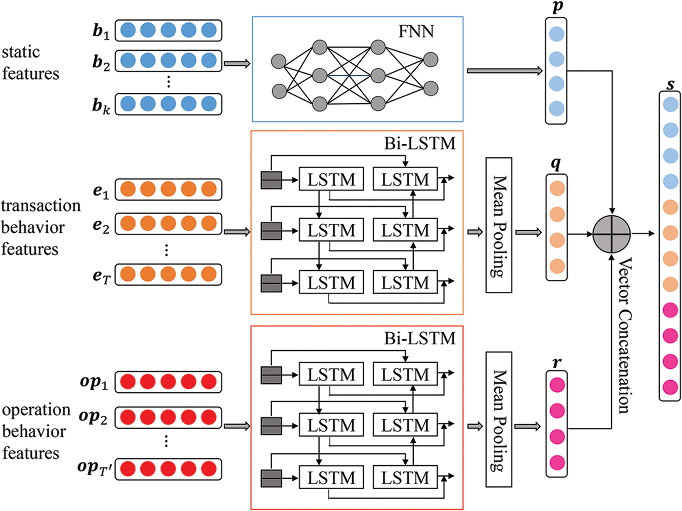
Figure 1: Structure of the multi-feature fusion module

3.1.1 FNN for Static Features Fusion

The set B=(b1,b2,⋯,bk) represents a cardholder’s static features, where each element b1,b2,⋯,bk in the set represents a static attribute of the cardholder, such as gender, occupation, marital status, etc. Each static attribute bi is mapped as a one-hot vector. Then, a FNN model is built with an input layer, an output layer, and three hidden layers with multiple neurons. The conversion and computation procedure from n−th layer neurons to (n+1)−th layer neurons is shown as Eq. (1).

xn+1=fn+1(Wn+1xn+φn+1)(1)

fn+1 is the activation function of the (n+1)−th layer neurons, Wn+1 is the weight matrix between the n−th layer neurons and the (n+1)−th layer neurons, and φ is the bias. By using the FNN model, the set B is transformed into a feature vector p, which helps to build a high-dimensional hidden representation between different static features. For example, a cardholder’s job may strongly correlate with his or her gender.

3.1.2 Bi-LSTM for Transaction Behavior Features Fusion

Jha et al. [3] aggregated transactions to capture the purchasing behavior of consumers prior to each transaction. This aggregated data was then used for model estimation to identify fraudulent transactions. They found that aggregated transaction behavior features were more helpful than raw transaction features. Referencing their research, this paper develops a Bi-LSTM model to capture the dynamic payment behavior of users over time and obtain the hidden state q.

The set E=(e1,e2,⋯,eT) is used to represent the sequence of a cardholder’s credit card transactions during a specific time period [1,T], E∈RK×T, where each element in E represents a transaction record of the cardholder at a specific time. Each transaction record contains K attributes, including transaction type, transaction amount, counterparty, etc. Each attribute represents a feature. ht′ is the representation vector of transaction behavior features for the cardholder at time t, and its calculation method is shown as Eq. (2), where ht→ is the output of the forward LSTM network and ht← is the output of the backward LSTM network. The operator ⊕ denotes concatenation.

ht′=[ht→⊕ht←], t∈[1,T](2)

At time t, et is the input data of the LSTM cell, ct is the value of the memory cell, ht is the output of the LSTM cell, and ht−1 is the output of the LSTM cell at the previous moment. The formula for the LSTM unit calculation method is as follows:

ct~=tanh(Wcet+Ucht−1+φc)(3a)

it=σ(Wiet+Uiht−1+φi)(3b)

ft=σ(Wfet+Ufht−1+φf)(3c)

ot=σ(Woet+Uoht−1+φo)(3d)

ct=ft⊙ct−1+it⊙ct~(3e)

ht=ot⊙tanh(ct)(3f)

Wc, Wi, Wf, and Wo represent the weight matrix, while φc, φi, φf, and φo represent the bias.

it, ft, and ot stand for the input gate vector, the forget gate vector, and the output gate vector of the dynamic payment behavior feature at time t, respectively. Lastly, a pooling layer is adopted to integrate the dynamic behavior features of all transactions for the cardholder in time T by the vector q.

q=1T∑t=1Tht′(4)

3.1.3 Bi-LSTM for Operation Behavior Features Fusion

The majority of credit card products and services in China are provided by banking institutions. Generally speaking, while using the credit card products of a bank, the cardholder will also use the debit card, e-bank, mobile banking, and other financial service products provided by the same bank. Therefore, in addition to the user’s credit card-related data, the issuing bank can also collect a large amount of operation behavior data about the user in other financial service channels, such as the user’s deposit and withdrawal records from Automated Teller Machines (ATM), transfer records through the e-bank, records of browsing financial information via the mobile banking app, etc. By adding this information about operations, the issuing bank can create a more accurate baseline for cardholders and find fraudulent transactions more easily.

The set O=(op1,op2,⋯,opT′) is used to represent the operation behavior sequence of cardholders in various financial service channels of the issuing bank within a specific time period [1, T′], O∈RK′×T′, where each element in O represents an operation record of the cardholder. Each operation record includes K′ attributes (such as time, channel type, operation type, etc.). Each attribute represents a feature. The operation behavior data is time series data, which is the same as transaction behavior data. Therefore, as shown in Eq. (5), this research constructs a Bi-LSTM network similar to the network structure described in Section 3.1.2 to embed the operation behavior sequence set O in a feature vector r.

r=Bi-LSTM(O)(5)

Finally, the static feature vector p, the transaction behavior feature vector q, and the operation behavior feature vector r are concatenated to form a unified high-dimensional feature representation vector s that integrates three types of features for the cardholder. The calculation is depicted in Eq. (6).

s=p⊕q⊕r(6)

3.2 Balance Module

To reduce the negative effect of the class imbalance problem on the performance of CCFD models, this paper presents a balance module based on BSMOTE and GAN to synthesize minority class samples. The data flow diagram of the balance module is shown in Fig. 2.

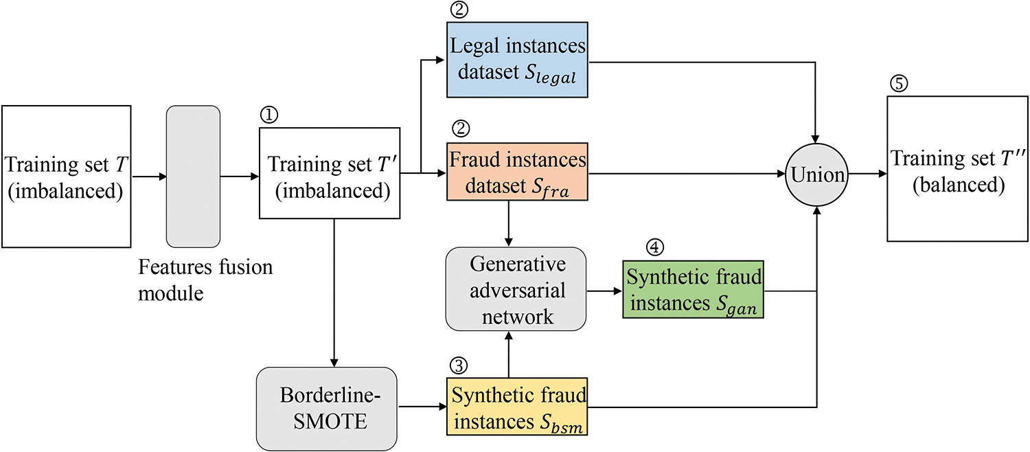
Figure 2: Data flow diagram of the balance module

In contrast to most previous research, the MFGAN model does not use GAN alone in the balance module, as experiments show that the performance of the resampling approach based on the combination of BSMOTE and GAN is better than that of the resampling method using only GAN. Details will be provided in the upcoming section on experiments and results.

3.2.1 BSMOTE

SMOTE and BSMOTE are famous resampling algorithms. The key steps of the SMOTE algorithm are as follows:

Step 1: For each sample xi from the minority class set Smin, randomly select a sample xneighbor from the k nearest neighbor samples from xi.

Step 2: Randomly select a point along the line connection samples xi and xneighbor to generate a new sample xnew. The procedure for calculating xnew is shown as Eq. (7), where λ is a random number.

Step 3: Repeat steps 1 and 2 until the desired number of minority samples have been synthesized.

xnew=xi+(xneighbor−xi)×λ, λ∈(0,1)(7)

The drawback of SMOTE is that the synthesized samples may weaken the boundary and increase the possibility of overlap between different classes in the original dataset, which may cause the model to misclassify boundary samples [36]. BSMOTE is optimized on the basis of SMOTE.

Firstly, BSMOTE divides the minority class into a “noise set,” a “safe set,” and a “dangerous set.” For each sample xi from the minority set Smin, the k nearest neighbor samples from xi are picked out from the training set S. xi is assigned to the “noise set” if the k samples are all majority samples. xi is assigned to the “safe set” if the number of majority samples among the k samples is less than k/2. Otherwise, xi is assigned to the “dangerous set.” Then, BSMOTE randomly selects xi′ from the “dangerous set” alone, which is different from the SMOTE method. Finally, a new sample is synthesized based on xi′.

3.2.2 Generative Adversarial Networks

The generative adversarial network consists of two modules: the generator G and the discriminator D. Typically, both G and D are deep neural networks [45]. G learns the probability distribution of actual samples and generates new candidate samples through the random noise input z. D judges whether or not a sample instance is synthesized by the generator. The goal of D is to distinguish actual samples from synthetic samples as accurately as possible, while the purpose of G is to generate instances that resemble actual samples to cheat D. In the procedure described above, G and D compete against each other and continuously improve their learning ability until a balance is reached. The discriminator D is trained to minimize its prediction error, and the generator G is trained to maximize the prediction error of D. The competition between G and D can be formalized as a minimax game, shown as Eq. (8).

minGmaxDV(D,G)=Ex∼pdata(x)[logD(x)]+Ez∼pz(z)[log(1−D(G(z)))](8)

pdata represents the distribution of actual samples, and pz represents the distribution of noise samples. In an ideal situation, after numerous iterations of training, each sample xg synthesized by the generator can perfectly trick the discriminator. This means that the discriminator cannot accurately distinguish whether xg is an actual sample or not. Maintaining a balance between the generator and discriminator is crucial to training a GAN. If the discriminator’s performance improves early, the generator will be unable to match the improved speed of the discriminator, resulting in the failure of the GAN’s training. Therefore, training a GAN is known to not be an easy task [20,46].

3.2.3 Balance Algorithm Based on BSMOTE and GAN

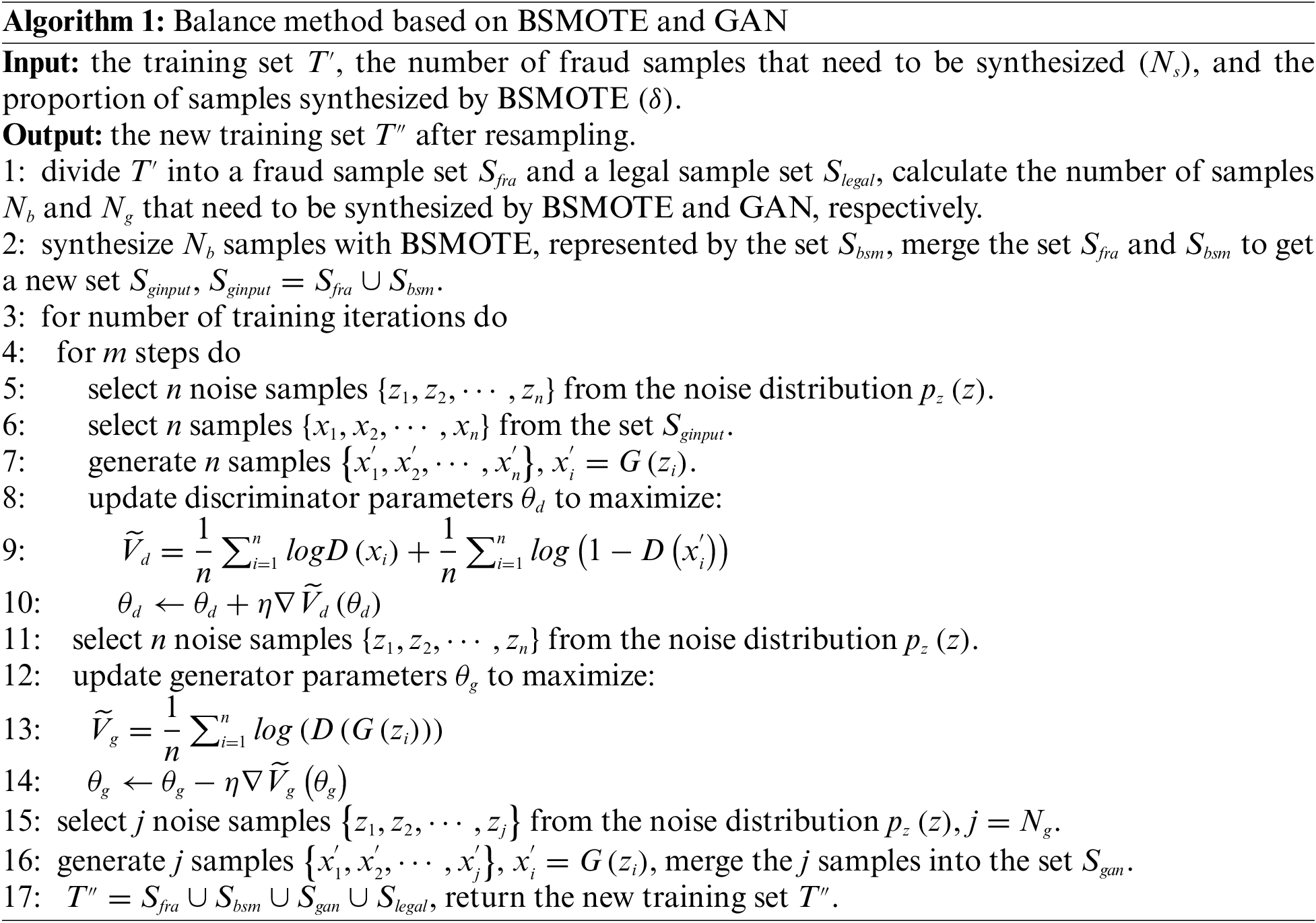
To compensate for the fact that the GAN method does not work well when there are not enough fraud samples, this work proposes a balance technique based on the combination of BSMOTE and GAN (as shown in Fig. 2). The balance algorithm mainly includes three steps. Firstly, the BSMOTE is used to synthesize a portion of instances to increase the number of fraud samples. Then, the actual and synthesized fraud samples are merged and used to train the GAN. Finally, a part of the fraud samples is generated by the GAN to make the training set class balanced. The detailed steps are as follows:

Step 1: The original imbalanced training set T is preprocessed by the multi-feature fusion module to produce the transformed training set T′, which is then split into a fraudulent sample set Sfra and a legitimate sample set Slegal.

Step 2: Using the training set T′ as input, the BSMOTE is utilized to synthesize Nb fraud samples, which are represented by the set Sbsm, and Nb=|Sbsm|.

Step 3: Feeding the actual fraud sample set Sfra and the synthetic fraud sample set Sbsm into the GAN, training the GAN until convergence, and then synthesizing Ng fraud samples by the generator of the GAN, which is represented by the set Sgan.

Step 4: Merging Sfra, Sbsm, Sgan, and Slegal to create a new balanced training set T″.

The pseudo-code of the balance method is shown in Algorithm 1.

4  Experiments

4.1 Dataset Description

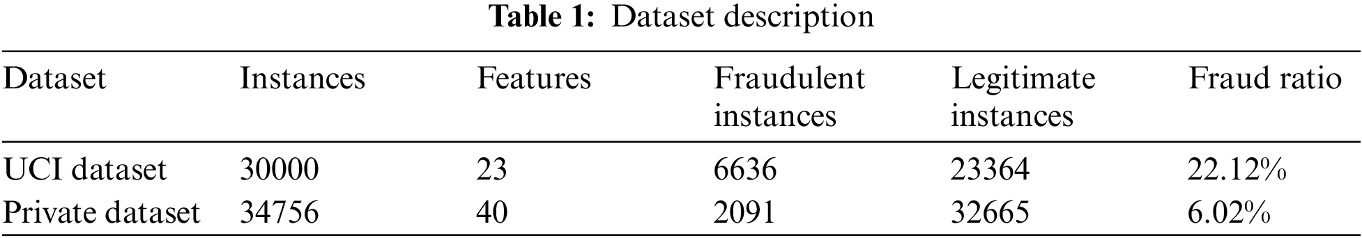
This research compares the performance of the proposed model and state-of-the-art models on two actual credit card datasets. The first is a public dataset from University of California, Irvine (UCI), while the second is a private dataset from a bank in China. Due to concerns about trade secrets and privacy, the provider of the private dataset did not explain in detail how the data was collected and how fraudulent transactions were labeled. They also did not illustrate how many fraudulent transactions actually happen in real business. Some statistical information about these two datasets is presented in Table 1.

(1)   The UCI dataset [47]. This dataset contains 30000 instances, 6636 of which are fraudulent and 23364 of which are legitimate. The fraud rate of the dataset is 22.12%. Each payment record has 23 features. There are five static features, like gender, education level, credit limit, etc., and 17 transaction behavior features, like the history of past payments, the amount of the billing statement, etc.

(2)   The private dataset. This dataset contains 34756 instances, including 2091 fraudulent instances and 32665 legitimate instances. The fraud rate is 6.02%, which shows that the dataset is highly imbalanced. Each instance of this dataset represents a customer’s credit card transaction record. Each record has 40 features, including eight static features (like age, gender, marital status, etc.) and 32 transaction behavior features (like the transaction amount, the number of transactions in the past 30 days, the average transaction amount in the past 30 days, etc.). In addition, the issuing bank provides 272584 records on cardholders’ operating behavior across various financial service channels. Each record is comprised of six attributes (such as customer ID, operation type, etc.). However, this part of the operation behavior data lacks labels, so it needs to be processed by hand before classification models can utilize it.

4.2 Performance Measures

The AUC of the receiver operating characteristic is often used to evaluate the performance of imbalanced classification models, such as in the studies by Douzas et al. [44] and Singla et al. [48]. In addition, AUC is usually applied in CCFD research. For example, Esenogho et al. [16] and Fang et al. [49] used AUC as the key performance indicator for their proposed models. This research adopted AUC, F1, recall, and precision as performance metrics to simplify comparisons with other baseline models and state-of-the-art models. The calculation methods for Recall, Precision, and F1 are depicted in Eqs. (9)–(11), where TP indicates a fraudulent transaction is predicted to be fraudulent, FP denotes a legal transaction is predicted to be fraudulent, and FN means a fraudulent transaction is predicted to be legal. Eq. (12) shows how to figure out AUC, where D+ and D− denote the collection of fraudulent transactions and legitimate transactions, respectively.

Recall=TPTP+FN(9)

Precision=TPTP+FP(10)

F1=2×Recall×PrecisionRecall+Precision(11)

AUC=1−1|D+|⋅|D−|∑x+∈D+∑x−∈D−(I(f(x+)<f(x−))+12I(f(x+)=f(x−)))(12)

4.3 Experimental Design

4.3.1 Baseline Methods

This paper constructs the following four baseline models based on the latest literature. It is well known that the setting of hyperparameters significantly impacts the performance of classification models. So, the grid search technique was used to set the hyperparameters of the model in this study to ensure that these baseline models can achieve the highest AUC and F1 on the validation dataset.

(1)   The DNN model. As the base classifier, a deep neural network model is built and combined with different balance techniques, such as SMOTE, BSMOTE, etc. The number of deep network layers is a basic hyperparameter. Models with too few layers are easy to be underfitting, while models with too many layers are easy to be overfitting. Five network structures with three to seven layers are evaluated, and the performance of the model is most stable when the number of layers is set to four.

(2)   The Support Vector Machine with Information Gain model (SVMIG). According to the method proposed by Poongodi et al. [9], a SVMIG model is constructed in this work. The input of the SVMIG model is the raw feature data without fusion.

(3)   The LSTM model. This paper implements a LSTM model with an attention mechanism according to the method presented by Benchaji et al. [17]. Then, the performance of the LSTM model is compared with that of the DNN model. The LSTM model contains six layers, and its input is the fused feature data.

(4)   The GAN model. Following the method described in the study by Fiore et al. [20], a GAN-based resampling module is constructed to replace the balance module of the MFGAN model. The generator and discriminator of the GAN model contain three layers, respectively. Except for the output layer, the number of neurons in other layers is 30 to 60.

4.3.2 Model Implementation and Experimental Details

(1)   The multi-feature fusion module. The FNN model for static feature fusion consists of four layers. There are five and seven layers in the Bi-LSTM models for transaction behavior and operation behavior feature fusion, respectively. The number of neurons in each layer is less than 100. Learning rates on a logarithmic grid (1 × 10−4, 5 × 10−3, and 1 × 10−3) are tested for different datasets.

(2)   The balance module. The generator G and the discriminator D are network structures with three layers. The number of neurons in each layer varies slightly according to the datasets used, but neither exceeds 80. Rectified Linear Unit (ReLU) and sigmoid are the activation functions of G and D, respectively. The model optimizers are Adams, and the learning rates of these two models are 1 × 10−4 and 5 × 10−3 on the UCI and private datasets, respectively. The hyperparameter δ is tuned in the range of [0.05, 0.5].

(3)   Dataset splitting. The original imbalanced dataset was split into two parts: 80% of it was training data (Str), and 20% was test data (Ste). Firstly, the balance module was used to optimize Str to generate a new training set (Str′). Secondly, the set Str′ was used to train the model and adjust its parameters. The five-fold cross-validation method was utilized to find the best classification model hyperparameters. Finally, the performance of different classification models is evaluated using the imbalanced set Ste.

(4)   Hardware and software environments for experimentation. All experiments in this paper were performed on a computer with 16 GB of RAM, a NVIDIA GeForce GTX 1080 Ti 11G GPU, and an Intel Core i7-9700 CPU @ 3.00 GHz running Windows 10 Professional with Python 3.6, Anaconda 4.5, and TensorFlow 2.4.

5  Experimental Results and Discussion

5.1 Comparative Analysis of the Results of MFGAN and Baseline Models

The experimental results are summarized in Table 2. DNN denotes that the raw data without feature fusion is used as the DNN model’s input. DNN (fus) indicates that the fused features of the dataset are obtained first, and then the fused features are used as the input of the DNN model. DNN (SMOTE) means that SMOTE is adopted to balance the training set. The following observations can be made based on the experimental outcomes of the UCI dataset:

(1)   For the raw data without feature fusion, SVMIG achieved a slightly higher recall rate than DNN, but its precision, F1 score, and AUC were lower than DNN’s (8.37% for precision, 4.57% for F1 score, and 2.6% for AUC). This indicated that DNN was better at fitting complex features than SVMIG.

(2)   The performance of DNN (fus) was better than that of DNN, in which the recall rate, precision, F1 score, and AUC were increased by 3.31%, 0.91%, 2.14%, and 1.45%, respectively. The results proved the effectiveness of the multi-feature fusion module from another aspect. For models that used fused features as input, the performance of LSTM (fus) and DNN (fus) was basically the same, and LSTM didn’t show a significant advantage.

(3)   DNN (fus, SMOTE) and DNN (fus, BSMOTE) models performed better than DNN (fus). When the SMOTE and BSMOTE algorithms were used to balance the training dataset, the recall rate of the DNN model increased by 1.86% and 3.22%, respectively, while the F1 score was not decreased. This indicated that the balance algorithm could help the classification model learn from minority samples better and make it more accurate for the minority samples to be identified.

(4)   The GAN model achieved the best recall rate (62%) and AUC (76.64%) among baseline models. Compared to DNN (fus, SMOTE) and DNN (fus, BSMOTE), the AUC of GAN improved by 1.46% and 1.22%, respectively, and the recall rate increased by 6.49% and 5.13%, respectively. This indicated that the minority samples synthesized by the balance module based on GAN were more consistent with the distribution of actual minority samples. In other words, the GAN model generated better fraud samples.

(5)   The accuracy of classification models decreased to varying degrees while resampling algorithms were used. Compared to the DNN (fus), the precision of the DNN (fus, SMOTE) and the DNN (fus, BSMOTE) decreased by 0.6% and 1.33%, respectively. Although the GAN and MFGAN models lost 4.92% and 4.49% of their precision, their recall rates increased by 8.35% and 11.41%, respectively. The direct and indirect reputational losses caused by misidentifying fraudulent transactions are far greater than the increased investigation costs resulting from misjudging legitimate transactions. Banks can accept a slight drop in precision while increasing the recall rate for fraudulent transactions. The recall rate improvement of MFGAN is 2.5 times that of the decrease in precision, which will help banks to reduce fraud losses.

(6)   The MFGAN model proposed in this study integrated the advantages of GAN and BSMOTE, alleviated the class imbalance problem in CCFD by synthesizing higher quality samples for the minority class, and achieved a more stable and better performance. MFGAN improved the recall rate, F1 score, and AUC by 3.06%, 1.34%, and 0.64% compared with the best baseline model. Compared with the classic balance algorithm SMOTE, it increased the recall rate, F1 score, and AUC by 9.55%, 1.38%, and 2.1%, respectively.

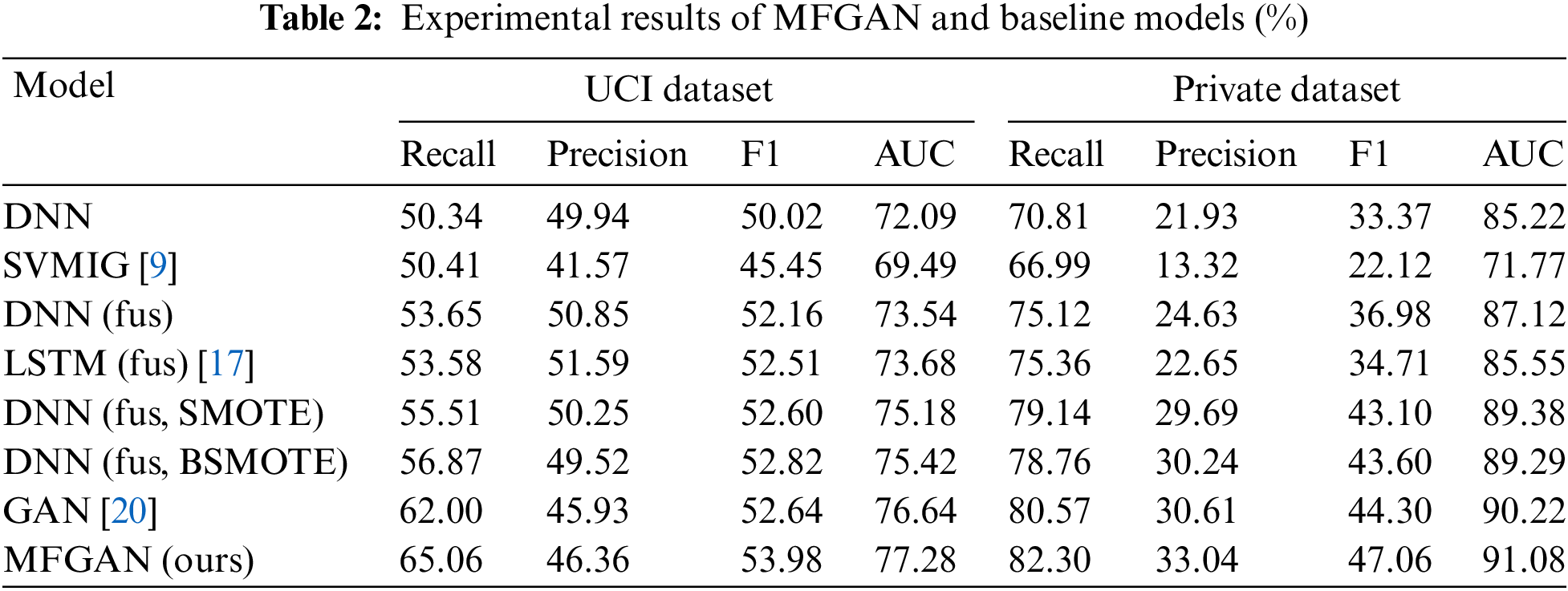
The experimental results of the private dataset showed a similar situation to that of the UCI dataset. The following points need to be noted:

(1)   Compared to DNN, DNN (fus) increased the recall rate, precision, F1 score, and AUC by 4.31%, 2.7%, 3.61%, and 1.9%, respectively, denoting that the fusion of different types of cardholder features contributed to improving the performance of the classification model. It also showed that the multi-feature fusion module could help classification models get a better and more unified representation of features than raw data.

(2)   After the training dataset was processed by balance methods, the recall rate, precision, and F1 score of the classification model were improved to varying degrees. For example, compared to DNN (fus), the recall rate, precision, and F1 score of the model with SMOTE increased by 4.02%, 5.06%, and 6.12%, respectively; the model with BSMOTE increased by 3.64%, 5.61%, and 6.62%, respectively; and the model with GAN performed better than both of them, reaching 5.45%, 5.98%, and 7.32%, respectively.

(3)   The MFGAN model achieved the best values on all evaluation metrics. Its recall rate, precision, F1 score, and AUC were 1.73%, 2.43%, 2.76%, and 0.86% higher than the GAN model, which obtained the best performance among baseline models. Compared to the traditional DNN model without feature fusion and class balance, the performance of MFGAN improved even more, reaching 11.49%, 11.11%, 13.69%, and 5.86% on the recall rate, precision, F1 score, and AUC, respectively.

5.2 Comparative Analysis of the Results with Different Numbers of Synthesized Samples

The balance module of MFGAN can create different training datasets with different balance ratios. This is done by setting the number of minority samples that need to be synthesized. In general, the balance ratios within the training dataset influence the performance of the classification model. So, it would be beneficial for banks to figure out how many synthesized samples should be added to the training set for the classification model to work best. For the UCI dataset, this work tested eight different numbers of synthetic samples Ng based on the number of fraudulent samples Nt within the training dataset, including 1/16, 1/8, 1/4, 1/2, 1, 3/2, and 2 times of Nt, and the number of samples that need to be synthesized to make classes balanced. The experimental results are shown in Tables 3 and 4. As shown in Fig. 3, the results are also presented as a line graph, which makes it easier to compare them.

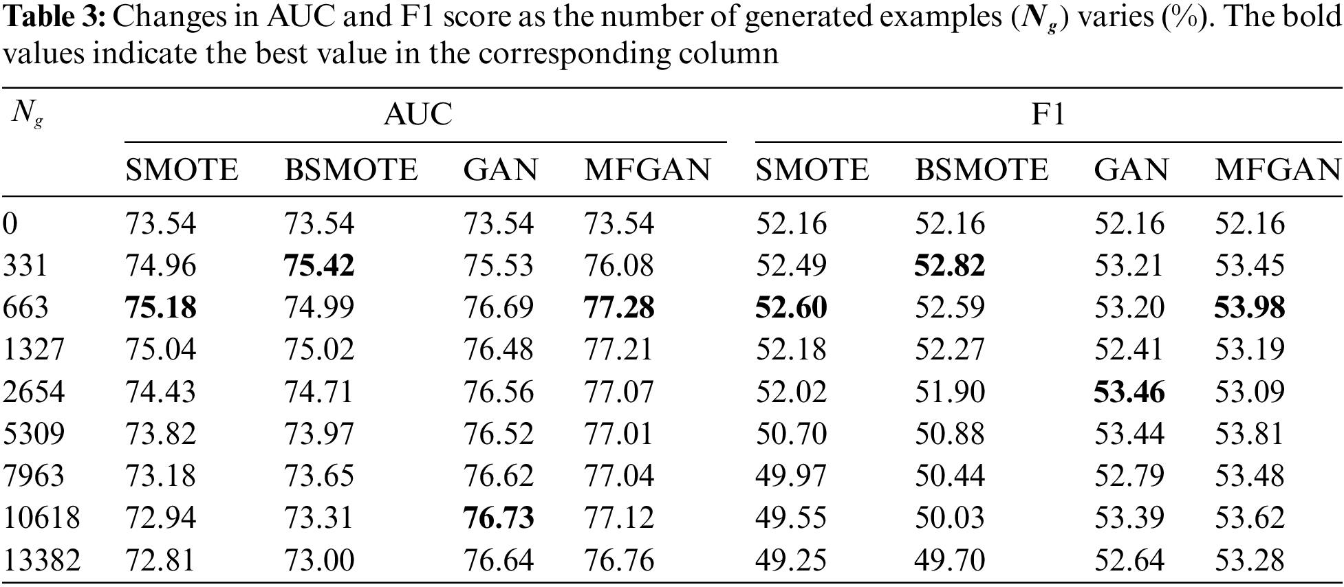
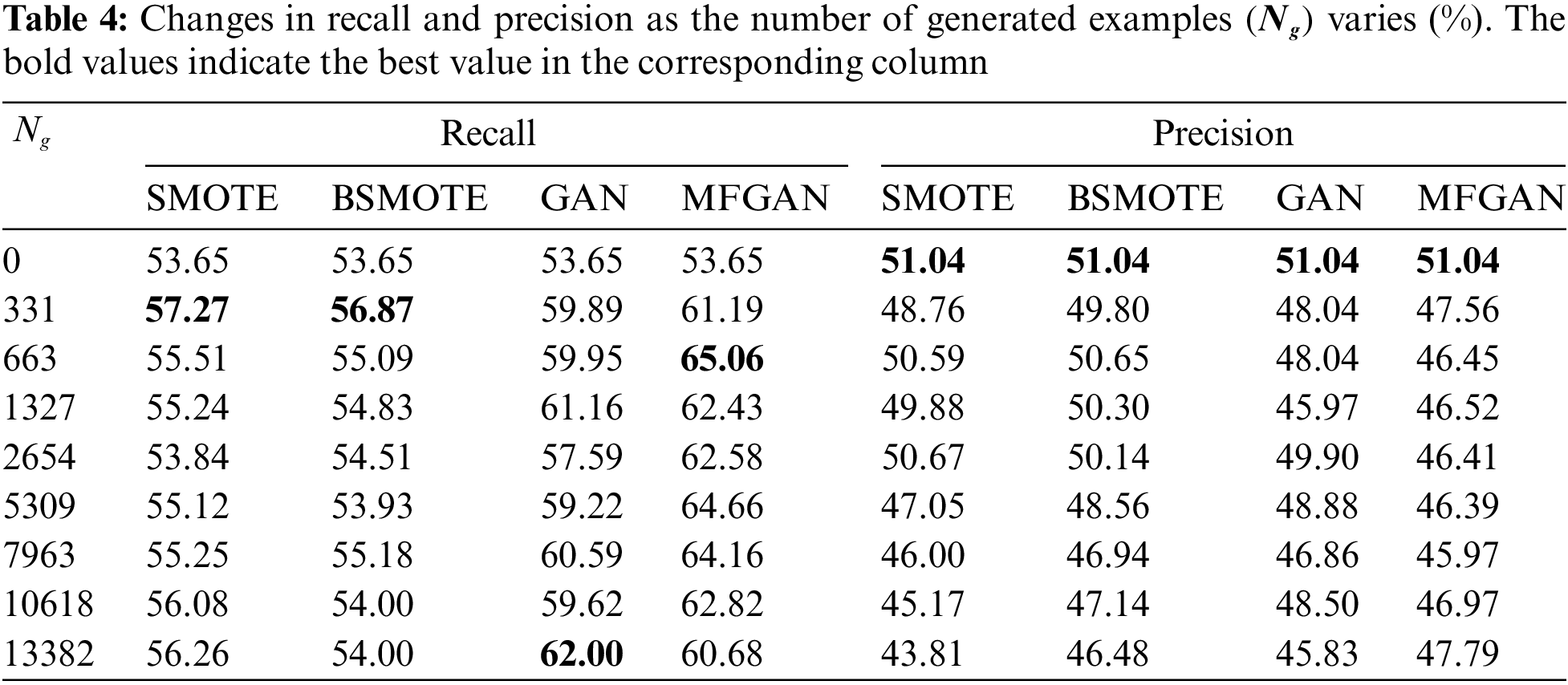
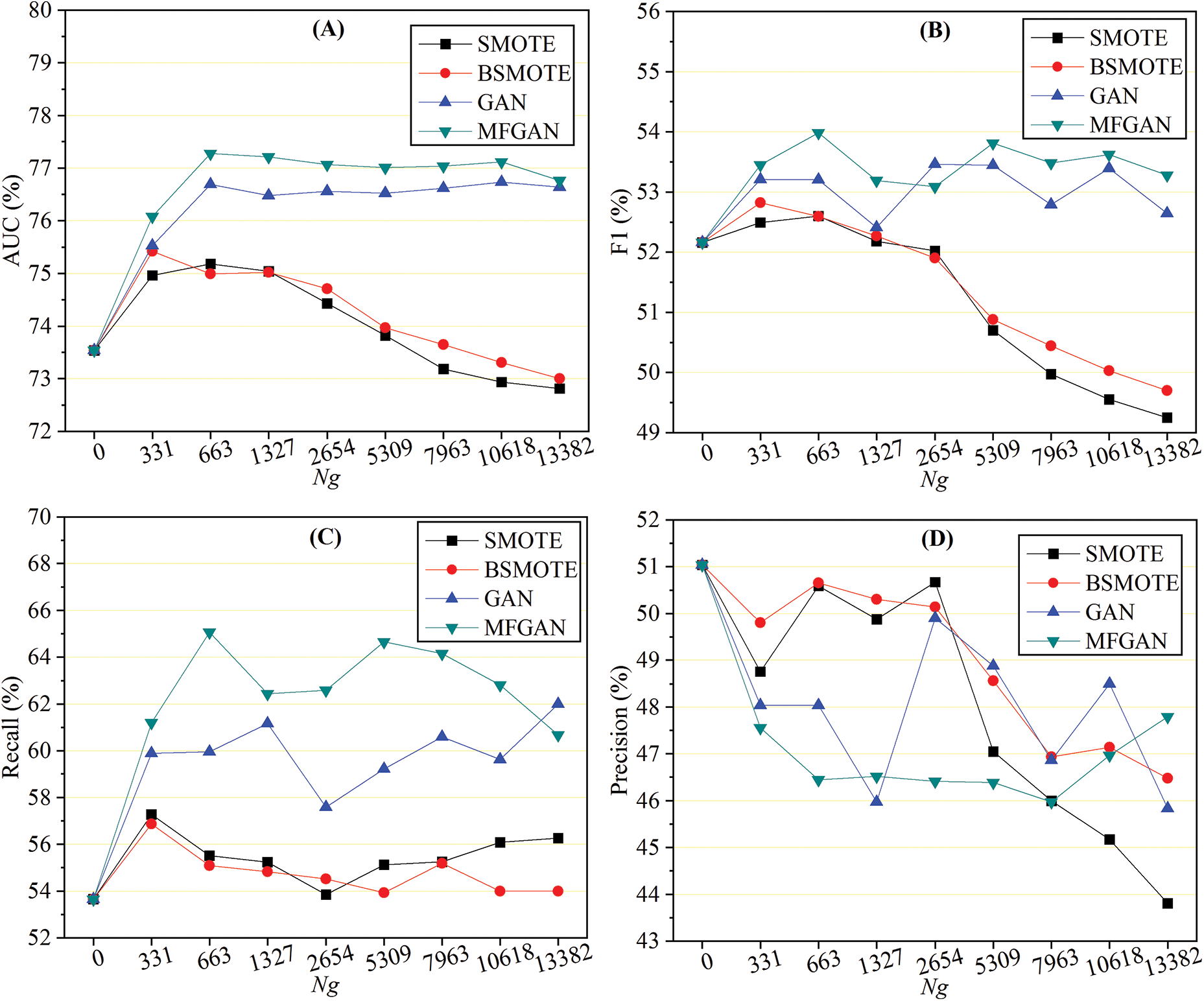
Figure 3: Performance with different numbers of samples generated: AUC (A), F1 (B), recall (C), and precision (D)

As shown in Fig. 3A, when an augmented training set was used, the AUC of GAN and MFGAN increased rapidly and then remained stable. At the same time, the AUC of SMOTE and BSMOTE began to decline after a slight increase. This indicated that the balance method based on generative adversarial networks was more stable in terms of AUC. For the F1 score, as depicted in Fig. 3B, the performance of models with SMOTE and BSMOTE grew slightly at first, then declined rapidly, and was much lower than the original F1 score when the class was balanced. This may be due to the fact that the balance algorithm synthesized a large number of noisy samples, which reduced the precision of the classification model for detecting fraudulent samples. The F1 scores of GAN and MFGAN presented a wave-like shape, rising first and then falling, but they were generally better than the original F1 score. As shown in Fig. 3C, the recall rate of the classification models was effectively improved when the training set was preprocessed by the balance method. SMOTE and BSMOTE improved recall rates less than MFGAN and GAN. In terms of precision, as shown in Fig. 3D, SMOTE and BSMOTE first fluctuated slightly and then dropped sharply after Ng = 2654. The stability of MFGAN was the best. After a significant decline in the initial phase, its precision tended to be stable and began to increase gradually in the last phase. All four resampling methods drop the precision metrics, but to different degrees. This may be because the original classification model shifted toward fraud samples when synthetic fraud samples were added, increasing the misclassification rate of the model for fraud transactions. It can be seen from Fig. 3 that the comprehensive performance of the MFGAN model was better than the other three models, and the best value was achieved when Ng was set to 1/8 times of Nt.

5.3 Ablation Study

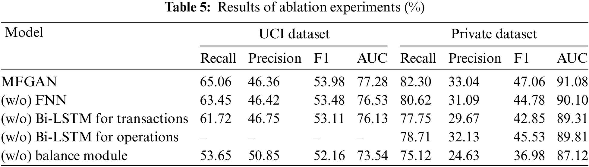
This research analyzed the contributions made by each component of the MFGAN model by performing ablation experiments on the UCI dataset and the private dataset. “(w/o) FNN” represents that the FNN model was removed from the multi-feature fusion module. This means that the raw data of cardholders’ static features was directly input into the classification model without fusing. “(w/o) Bi-LSTM for transactions” indicates that the Bi-LSTM model used to fuse transaction behavior data of cardholders was removed from the multi-feature fusion module; that is, the raw transaction behavior data was directly fed into the classification model. “(w/o) Bi-LSTM for operations” means that the operation behavior data of cardholders was not fused. This part of the raw data was not input into the classification model because it was too large and lacked labels. “(w/o) balance module” specifies that the balance module was removed from the MFGAN model, leaving the imbalanced training set to be directly input into the classification model.

Table 5 shows the results of the ablation experiment. Because the UCI dataset doesn’t have any information about cardholders’ operation behavior, “–” is used to indicate the result of this item in the ablation experiment. The results of the experiments show that the balance module helped the classification model improve its performance in a big way. For example, in terms of recall rate, the model with the balance module was improved by 11.41% and 7.18% on the UCI and the private datasets, respectively. In addition, fusing three different types of feature data could also improve the model’s performance to varying degrees, proving that the multi-feature fusion module could help the model extract advanced hidden features of cardholders from different data. For example, when operational behavior data was integrated into the input data, the model’s recall rate, precision, F1 score, and AUC on the private dataset were improved by 3.59%, 0.91%, 1.53%, and 1.27%, respectively.

6  Conclusion

This paper proposed a novel credit card fraud detection model called MFGAN. The MFGAN mode was made up of two modules: a fusion module for extracting advanced hidden features from multi-source heterogeneous data and a balance module for alleviating the problem of class imbalance. In the multi-feature fusion module, three neural network models were built to process the static and dynamic features of cardholders, respectively. In addition, the operation behavior data of cardholders in different financial service channels was also utilized in this study, which was rarely addressed in other recent CCFD literature for reasons such as user privacy protection and a lack of data. In the balance module, a resampling algorithm based on the generative adversarial network and BSMOTE was proposed. Compared to state-of-the-art resampling methods, the proposed algorithm could synthesize better minority samples and help the classification model improve its performance. Lastly, experiments were conducted on two real-world credit card datasets, and how the performance changes with the number of synthesized minority samples were also investigated. The experimental results showed that, compared to state-of-the-art models, the MFGAN model achieved a higher AUC and recall rate without reducing the F1 score, which proved that the MFGAN model was feasible and effective.

There are some flaws in this paper. For example, the fusion module will diminish the interpretability of the model, and the model doesn’t take into account the influence of concept drift problems [50], like changes in fraudulent behavior over time. Therefore, the MFGAN model needs some targeted improvements before it can be put into production as the bank’s anti-fraud system. In the future, an adaptive module of concept drift will be designed to make the proposed approach more stable when fraud behavior changes.

The main contributions of this study are as follows: First, a multi-feature fusion method is proposed to address the issue of insufficient feature extraction and representation in CCFD. Second, an upsampling method based on GAN and BSMOTE is proposed as a solution to the class imbalance problem. Third, the effectiveness of the proposed model is validated using two real-world credit card datasets.

Acknowledgement: The authors wish to acknowledge the contribution of Basic Software Engineering Research Center of NUDT.

Funding Statement: This work was partially supported by the National Key R&D Program of China (Nos. 2022YFB3104103, and 2019QY1406) and the National Natural Science Foundation of China (Nos. 61732022, 61732004, 61672020, and 62072131).

Author Contributions: The authors confirm contribution to the paper as follows: study conception and design: Yalong Xie, Aiping Li; experiments and interpretation of results: Yalong Xie, Liqun Gao, Hongkui Tu; draft manuscript preparation: Yalong Xie, Biyin Hu. All authors reviewed the results and approved the final version of the manuscript.

Availability of Data and Materials: The data and materials used to support the findings of this study are available from the corresponding author upon request.

Conflicts of Interest: The authors declare that they have no conflicts of interest to report regarding the present study.

References

1. C. V. Priscilla and D. P. Prabha, “Influence of optimizing xgboost to handle class imbalance in credit card fraud detection,” in Proc. of ICSSIT, Tirunelveli, India, pp. 1309–1315, 2020. [Google Scholar]

2. A. Singh and A. Jain, “An empirical study of aml approach for credit card fraud detection-financial transactions,” International Journal of Computers Communications & Control, vol. 14, no. 6, pp. 670–690, 2020. [Google Scholar]

3. S. Jha, M. Guillen and J. C. Westland, “Employing transaction aggregation strategy to detect credit card fraud,” Expert Systems with Applications, vol. 39, no. 16, pp. 12650–12657, 2012. [Google Scholar]

4. S. Bhattacharyya, S. Jha, K. Tharakunnel and J. C. Westland, “Data mining for credit card fraud: A comparative study,” Decision Support Systems, vol. 50, no. 3, pp. 602–613, 2011. [Google Scholar]

5. A. S. Hussein, R. S. Khairy, S. M. M. Najeeb and H. T. S. Alrikabi, “Credit card fraud detection using fuzzy rough nearest neighbor and sequential minimal optimization with logistic regression,” International Journal of Interactive Mobile Technologies, vol. 15, no. 5, pp. 24–41, 2021. [Google Scholar]

6. Y. Sahin, S. Bulkan and E. Duman, “A cost-sensitive decision tree approach for fraud detection,” Expert Systems with Applications, vol. 40, no. 15, pp. 5916–5923, 2013. [Google Scholar]

7. D. Zhang, X. Zhou, S. C. H. Leung and J. Zheng, “Vertical bagging decision trees model for credit scoring,” Expert Systems with Applications, vol. 37, no. 12, pp. 7838–7843, 2010. [Google Scholar]

8. N. Rtayli and N. Enneya, “Enhanced credit card fraud detection based on svm-recursive feature elimination and hyper-parameters optimization,” Journal of Information Security and Applications, vol. 55, pp. 102596, 2020. [Google Scholar]

9. K. Poongodi and D. Kumar, “Support vector machine with information gain based classification for credit card fraud detection system,” International Arab Journal of Information Technology, vol. 18, no. 2, pp. 199–207, 2021. [Google Scholar]

10. C. Li, N. Ding, Y. Zhai and H. Dong, “Comparative study on credit card fraud detection based on different support vector machines,” Intelligent Data Analysis, vol. 25, no. 1, pp. 105–119, 2021. [Google Scholar]

11. P. Sharma, S. Banerjee, D. Tiwari and J. C. Patni, “Machine learning model for credit card fraud detection-a comparative analysis,” International Arab Journal of Information Technology, vol. 18, no. 6, pp. 789–796, 2021. [Google Scholar]

12. R. B. Asha and K. R. Suresh Kumar, “Credit card fraud detection using artificial neural network,” Global Transitions Proceedings, vol. 2, no. 1, pp. 35–41, 2021. [Google Scholar]

13. T. Sun and M. A. Vasarhelyi, “Predicting credit card delinquencies: An application of deep neural networks,” Intelligent Systems in Accounting, Finance and Management, vol. 25, no. 4, pp. 174–189, 2018. [Google Scholar]

14. X. Zhang, Y. Han, W. Xu and Q. Wang, “Hoba: A novel feature engineering methodology for credit card fraud detection with a deep learning architecture,” Information Sciences, vol. 557, pp. 302–316, 2021. [Google Scholar]

15. F. K. Alarfaj, I. Malik, H. U. Khan, N. Almusallam, M. Ramzan et al., “Credit card fraud detection using state-of-the-art machine learning and deep learning algorithms,” IEEE Access, vol. 10, pp. 39700–39715, 2022. [Google Scholar]

16. E. Esenogho, I. D. Mienye, T. G. Swart, K. Aruleba and G. Obaido, “A neural network ensemble with feature engineering for improved credit card fraud detection,” IEEE Access, vol. 10, pp. 16400–16407, 2022. [Google Scholar]

17. I. Benchaji, S. Douzi, B. E. Ouahidi and J. Jaafari, “Enhanced credit card fraud detection based on attention mechanism and lstm deep model,” Journal of Big Data, vol. 8, no. 1, pp. 151, 2021. [Google Scholar]

18. F. Carcillo, Y. L. Borgne, O. Caelen, Y. Kessaci, F. Oblé et al., “Combining unsupervised and supervised learning in credit card fraud detection,” Information Sciences, vol. 557, pp. 317–331, 2021. [Google Scholar]

19. J. Forough and S. Momtazi, “Ensemble of deep sequential models for credit card fraud detection,” Applied Soft Computing, vol. 99, pp. 106883, 2021. [Google Scholar]

20. U. Fiore, A. D. Santis, F. Perla, P. Zanetti and F. Palmieri, “Using generative adversarial networks for improving classification effectiveness in credit card fraud detection,” Information Sciences, vol. 479, pp. 448–455, 2019. [Google Scholar]

21. A. K. Gangwar and V. Ravi, “WiP: Generative adversarial network for oversampling data in credit card fraud detection,” in Proc. of ICISS, Tokyo, TKY, Japan, pp. 123–134, 2019. [Google Scholar]

22. N. Japkowicz and S. Stephen, “The class imbalance problem: A systematic study,” Intelligent Data Analysis, vol. 6, no. 5, pp. 429–449, 2002. [Google Scholar]

23. H. He and E. A. Garcia, “Learning from imbalanced data,” IEEE Transactions on Knowledge and Data Engineering, vol. 21, no. 9, pp. 1263–1284, 2009. [Google Scholar]

24. Z. Li, M. Huang, G. Liu and C. Jiang, “A hybrid method with dynamic weighted entropy for handling the problem of class imbalance with overlap in credit card fraud detection,” Expert Systems with Applications, vol. 175, pp. 114750, 2021. [Google Scholar]

25. E. Ileberi, Y. Sun and Z. Wang, “Performance evaluation of machine learning methods for credit card fraud detection using smote and adaboost,” IEEE Access, vol. 9, pp. 165286–165294, 2021. [Google Scholar]

26. J. R. Dorronsoro, F. Ginel, C. Sgnchez and C. S. Cruz, “Neural fraud detection in credit card operations,” IEEE Transactions on Neural Networks, vol. 8, no. 4, pp. 827–834, 1997. [Google Scholar] [PubMed]

27. A. C. Bahnsen, D. Aouada, A. Stojanovic and B. Ottersten, “Feature engineering strategies for credit card fraud detection,” Expert Systems with Applications, vol. 51, pp. 134–142, 2016. [Google Scholar]

28. Y. Lucas, P. Portier, L. Laporte, L. He-Guelton, O. Caelen et al., “Towards automated feature engineering for credit card fraud detection using multi-perspective hmms,” Future Generation Computer Systems, vol. 102, pp. 393–402, 2020. [Google Scholar]

29. D. J. N. J. Soemers, T. Brys, K. Driessens, M. H. M. Winands and A. Nowé, “Adapting to concept drift in credit card transaction data streams using contextual bandits and decision trees,” in Proc. of IAAI, Louisiana, LA, USA, pp. 7831–7836, 2018. [Google Scholar]

30. A. A. Taha and S. J. Malebary, “An intelligent approach to credit card fraud detection using an optimized light gradient boosting machine,” IEEE Access, vol. 8, pp. 25579–25587, 2020. [Google Scholar]

31. E. Kim, J. Lee, H. Shin, H. Yang, S. Cho et al., “Champion-challenger analysis for credit card fraud detection: Hybrid ensemble and deep learning,” Expert Systems with Applications, vol. 128, pp. 214–224, 2019. [Google Scholar]

32. J. Forough and S. Momtazi, “Sequential credit card fraud detection: A joint deep neural network and probabilistic graphical model approach,” Expert Systems, vol. 39, no. 1, pp. 12795, 2022. [Google Scholar]

33. Z. Li, G. Liu and C. Jiang, “Deep representation learning with full center loss for credit card fraud detection,” IEEE Transactions on Computational Social Systems, vol. 7, no. 2, pp. 569–579, 2020. [Google Scholar]

34. D. Jensen, “Prospective assessment of AI technologies for fraud detection: A case study,” in Proc. of AAAI, Rhode Island, RI, USA, pp. 34–38, 1997. [Google Scholar]

35. N. V. Chawla, K. W. Bowyer, L. O. Hall and W. P. Kegelmeyer, “SMOTE: Synthetic minority over-sampling technique,” Journal of Artificial Intelligence Research, vol. 16, no. 1, pp. 321–357, 2002. [Google Scholar]

36. H. Han, W. Wang and B. Mao, “Borderline-smote: A new over-sampling method in imbalanced data sets learning,” in Proc. of ICIC, Hefei, China, pp. 878–887, 2005. [Google Scholar]

37. A. Iranmehr, H. Masnadi-Shirazi and N. Vasconcelos, “Cost-sensitive support vector machines,” Neurocomputing, vol. 343, pp. 50–64, 2019. [Google Scholar]

38. S. Makki, Z. Assaghir, Y. Taher, R. Haque, M. Hacid et al., “An experimental study with imbalanced classification approaches for credit card fraud detection,” IEEE Access, vol. 7, pp. 93010–93022, 2019. [Google Scholar]

39. Y. Xie, A. Li, L. Gao and Z. Liu, “A heterogeneous ensemble learning model based on data distribution for credit card fraud detection,” Wireless Communications and Mobile Computing, vol. 2021, pp. 2531210, 2021. [Google Scholar]

40. S. Akila and U. S. Reddy, “Cost-sensitive risk induced Bayesian inference bagging (RIBIB) for credit card fraud detection,” Journal of Computational Science, vol. 27, pp. 247–254, 2018. [Google Scholar]

41. F. Shen, X. Zhao, G. Kou and F. E. Alsaadi, “A new deep learning ensemble credit risk evaluation model with an improved synthetic minority oversampling technique,” Applied Soft Computing, vol. 98, pp. 106852, 2021. [Google Scholar]

42. K. Niu, Z. Zhang, Y. Liu and R. Li, “Resampling ensemble model based on data distribution for imbalanced credit risk evaluation in P2P lending,” Information Sciences, vol. 536, pp. 120–134, 2020. [Google Scholar]

43. I. J. Goodfellow, J. Pouget-Abadie, M. Mirza, B. Xu, D. Warde-Farley et al., “Generative adversarial nets,” in Proc. of NIPS, Montreal, MTL, Canada, pp. 2672–2680, 2014. [Google Scholar]

44. G. Douzas and F. Bacao, “Effective data generation for imbalanced learning using conditional generative adversarial networks,” Expert Systems with Applications, vol. 91, pp. 464–471, 2018. [Google Scholar]

45. Y. LeCun, Y. Bengio and G. Hinton, “Deep learning,” Nature, vol. 521, no. 7553, pp. 436–444, 2015. [Google Scholar] [PubMed]

46. M. Arjovsky and L. Bottou, “Towards principled methods for training generative adversarial networks,” in Proc. of ICLR, Toulon, TOU, France, pp. 1–17, 2017. [Google Scholar]

47. UC Irvine machine learning repository, “Default of credit card clients data set,” 2016. [Online]. Available: https://archive.ics.uci.edu/ml/datasets/default+of+credit+card+clients [Google Scholar]

48. K. J. Singla, A. Kashif Bashir, Y. Nam, N. UI Hasan et al., “Handling class imbalance in online transaction fraud detection,” Computers, Materials & Continua, vol. 70, no. 2, pp. 2861–2877, 2022. [Google Scholar]

49. Y. Fang, Y. Zhang and C. Huang, “Credit card fraud detection based on machine learning,” Computers, Materials & Continua, vol. 61, no. 1, pp. 185–195, 2019. [Google Scholar]

50. R. F. Mansour, S. Al-Otaibi, A. Al-Rasheed, H. Aljuaid, I. V. Pustokhina et al., “An optimal big data analytics with concept drift detection on high-dimensional streaming data,” Computers, Materials & Continua, vol. 68, no. 3, pp. 2843–2858, 2021. [Google Scholar]