Dendritic Cell Algorithm with Bayesian Optimization Hyperband for Signal Fusion

1  Introduction

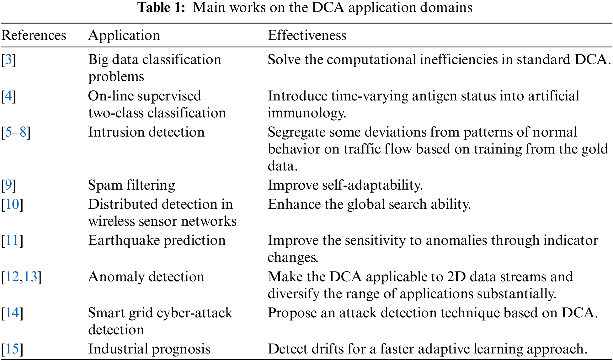
The DCA is one of the prevailing paradigms in the artificial immune system, which is inspired by the functioning of the biological dendritic cells (DCs) [1]. The DCs traverses the tissue to gather the information (signals) around, which is namely the pathogenic associated molecular patterns (PAMP), safe signals (SS), and danger signals (DS) in immunology [2]. The primary purpose of DCs is to present a decision on whether these organizations are dangerous or safe by fusing these signals. DCA mimics the antigen presentation process of DCs to perform the fusion of real-valued input data and correlates those combined data with the data class to form a binary classifier. As an excellent prototype for developing Machine Learning, DCA has been widely applied in classification [3,4], intrusion detection [5–8], spam filtering [9], distributed and parallel operations [10], earthquake prediction [11], anomaly detection [12,13], cyber-attack detection in smart grid [14], and industrial prognosis [15]. Table 1 lists the application domains and effectiveness of DCA. Current research on the DCA has shown that the algorithm not only exhibits excellent detection accuracy but is also expected to help reduce the rate of misclassification and false alarms that occur in similar systems.

Due to many tunable parameters, the classical DCA received a lot of criticism [16]. The reason is that selecting these parameters is a stochastic process that brings various sources of uncertainty into the algorithm. The classical DCA relies on expert knowledge to set these parameter values. The reliance on expertise is undesirable and receives the criticism of having over-fitted the data to the algorithm. Therefore, many researchers focus on how to reduce the uncertainty of DCA. Several researchers devoted themselves to reducing the parameters in DCA, and some studied the influence of parameters on the algorithm through experiments and mathematical reasoning.

Greensmith et al. [17] proposed a deterministic DCA (dDCA) with less tunable parameters than classical DCA to reduce uncertainty. Greensmith et al. [18] presented a deterministic DCA version, namely hDCA, to describe dDCA in Haskell by purely functional programming to solve the previous inaccuracies in portraying the algorithm. Mukhtar et al. [19] proposed a fuzzy dDCA (FdDCA), which combines dDCA, fuzzy sets, and K-means clustering to construct a signal fusion function. The approach employed k-means clustering and a trapezoidal function to construct a membership function for classifying the cumulative signals into three concentration levels, low, medium, and high. And then, a rule and center of gravity were adopted to compute a crisp value for context assessment as the results of signal fusion. They utilized fuzzy sets and K-means clustering to replace the discriminating cumulative signals in the signal fusion function. This approach may only sometimes lead to satisfactory results for DCA due to relying on human experience to construct the signal fusion function.

It’s challenging to confirm which parts of the system are responsible for what aspects of the algorithm’s function. Musselle [20] studied the migration threshold, a parameter in dDCA, and tested versions of the standard dDCA with differing values for the migration threshold. Their experiments showed that the standard dDCA with higher values of migration threshold could mitigate the errors. Greensmith [21] evaluated the influence of the migration threshold parameter in dDCA to move the DCA toward implementing a learning mechanism. And other researchers examined the DCA from a mathematical perspective. Stibor et al. [22] adopted the dot product to represent the signal fusion of the DCA. They proved that the signal fusion element of the DCA is a collection of linear classifiers. In view of the linear nature [23], Zhou et al. presented an immune optimization-inspired dDCA (IO-dDCA), which builds an artificial immune optimization mechanism for dDCA inspired by a nonlinear dynamic model and gradient descent. However, the dDCA has not been fully studied, and the underlying mathematical mechanism for classification is poorly understood. The IO-dDCA is highly effective for solving a convex function but is difficult to converge on non-convex functions. Therefore, the IO-dDCA based on gradient descent can only sometimes find the optimal global parameter configuration. The reason is that the classification process can’t be determined as a convex function.

Moreover, several researchers applied the popular search optimization tool to search the optimal DCA parameters. Elisa et al. [24] utilized a genetic algorithm (GA) as a search engine to find the optimal parameter configuration and proposed an extended DCA version, GADCA, related to signal fusion. Among these methods, some reduce the parameters and complexity of the algorithmic process; some construct signal fusion function by undesirable expertise; some introduce the nonlinear dynamic model and gradient descent to optimize parameters and ignore the case of non-convex functions; others rely on heuristic optimization algorithms, the time-consuming process needs enough initial samples.

Due to a poor understanding of the underlying classification mechanism, the loss function of DCA is ambiguous, and its gradients are difficult to access. Choosing the optimal parameter configuration is a problem. Motivated to optimize the parameters of DCA, this study models the parameters optimization as a black-box optimization. The black-box optimization aims to optimize an objective function f: X→R without any other information about the function f [25]. This black-box optimization property is desirable for parameter optimization in DCA with an inexplicit loss function. There are many techniques to be developed for black-box optimization, including random searching [26], grid searching [27], heuristic searching [28], BO [29], and multi-fidelity optimization (MFO) [30,31]. Random-searching and grid-searching are widely used in parameter optimization but are often considered brute-force methods. Classical heuristic search approaches have also been investigated, such as particle swarm optimization [28] and differential evolution [32,33]. Those methods have been broadly used to solve the numerical optimization problem, e.g., hyper-parameter optimization, job-shop scheduling problems, and multi-objective fuzzy job-shop scheduling problem. However, these heuristic search approaches require the entire data sets to evaluate a potential configuration rather than dynamically allocating appropriate budget to configurations. Generally, the budget for configurations in the early stage of the search process is the same as the valuable ones in the later process to estimate the scores of the configurations. The strategy is time-consuming, and can easily cause a waste of resources. To reduce running time, assorted variants of MFO are proposed, such as successive halving and hyperband, which allocate more resources to promising configurations and eliminate poor ones. To develop more efficient optimization methods, the problem has recently been dominated by BO. BO is a powerful technique that can directly model the expensive black-box function and is widely applied to tune parameters. The core of BO is to choose a minimum number of data points to make an informed choice. Typically, BO is given a fixed number of iterations without any awareness of the evaluation cost. It is prohibitive and undesired in real-world problems. Falkner et al. [25] proposed a new and versatile tool, BOHB, for parameter optimization, which comes with substantial speedups by combining hyperband [34] with BO. The BOHB relies on hyperband to determine the budget for each configuration and employs BO to select the most promising configurations replacing the original random selection in each iteration of the hyperband. Due to its excellent optimization capabilities, this study proposed a novel DCA expansion for signal fusion, BHDCA, which applies BOHB to optimize the parameters of DCA. This approach can find the optimal parameters for DCA without any details of the loss function while keeping the computation lightweight. The main contributions are as follows.

•   Firstly, this study provides formal definitions of the DCA through Haskell functional language to make researchers understand the algorithm better.

•   Secondly, this study models the parameter configuration and corresponding performance of DCA as a gaussian process because of the lack of comprehensive research on the classification mechanism. The BO is utilized to model the distribution of parameter configurations and the corresponding loss of DCA to choose the most promising potential configurations. To better reduce the resource consumption of the training process, this study applies hyperband to allocate an appropriate budget for each configuration. A novel BHDCA is presented, which employs BO and hyperband to optimize the parameters of DCA without knowing the gradient or details of the loss function. Therefore, this approach can efficiently accomplish parameter optimization while finding a trade-off between the budget and the optimal configuration.

•   Finally, the state-of-the-art DCA expansion algorithms for signal fusion (e.g., dDCA, FdDCA, GADCA, IO-dDCA) are discussed and compared with BHDCA on the University of California Irvine (UCI) Machine Learning Repository [35] and Keel-dataset Repository [36]. The experiment results and performance analysis show the effectiveness of BHDCA.

This paper is structured as follows: Section 2 describes the definitions of the DCA; the novel DCA extended, BHDCA, is proposed in Section 3; our following experiment setup, results, and analysis are described in Section 4; conclusions and future work are shown in Section 5.

2  Preliminary

2.1 Basic Definition

In the algorithm, each data item of DCA contains two inputs: signals and antigens. The antigen is the identifier of the data item, in other words, the data item IDs. The input signals have only three categories corresponding to the three immune signals, PAMP, SS, and DS. Each data item is transformed into the three input signals through a data pre-processing procedure. The DCA maintains a population of detectors, namely DCs. The DCs simulate the function of dendritic cells as a classifier to detect whether a data item is normal or abnormal. Each data item is processed by detectors selected from the population randomly. Finally, the algorithm synthesizes the detection results generated by DCs to label the data item as normal or abnormal.

Definition 1 An antigen is presented as Ag= <e,t>, e is the identifier of a certain data item to be detected, t is the timestamp.

Definition 2 The signal is denoted as Signal= <PAMP,DS,SS>, a 3-dimensional real valued tuple. SS is the safe signal value, DS is the danger signal value, PAMP is the value of pathogen-associated molecular patterns.

Definition 3 The DCA is described as HDCA=(IDCA,ODCA,FDCA), the IDCA is the input data including two components: Ags and Signals; the ODCA is the output of the DCA, either normal or abnormal; the FDCA represents the relationship between IDCA and ODCA, as shown in Eq. (1).

ODCA=FDCA(IDCA)={0,normal1,abnormal(1)

where ODCA is the output of DCA with the binary value 0 or 1, IDCA is the input of DCA including Ags and Signals, FDCA is the function of the mapping relationship between IDCA and ODCA.

2.2 The DCA

The DCA contains three main components: antigen sampling mechanism, signal fusion function, and output calculation. The antigen sampling mechanism generates the three input signals from the original data item. There are plenty of uncertainties in the whole operation of the DCA. The DCA maintains a population of DCs that detect data items as detectors and combines all the detecting results to determine whether the data class is normal or abnormal. For each input IDCA,i= <Agi,Signali>, the DCA randomly chooses several DCs to sample its signal values at the same time step; and calculates the three interim signals, known as the costimulatory molecule signal value (CSM), the semi-mature signal value (SEMI), and the mature signal value (MAT), through signal fusion function FDCA for each DC. Each DC can sample T inputs IDCA,i= <Agi,Signali> and accumulate their interim signals through the signal fusion function FDCA, as shown in Eq. (2). The three interim signals of each DC are continuously accumulated during the process of antigen sampling until reaching the condition for stopping sampling.

(CSM,SEMI,MAT)=∑i=1TWPAMP×SignalPAMP,iWPAMP+WDS+WSS+∑i=1TWDS×SignalDS,iWPAMP+WDS+WSS+∑i=1TWSS×SignalSS,iWPAMP+WDS+WSS(2)

where the SignalPAMP,i is the ith value of input signal PAMP, the SignalDS,i is the ith value of input signal DS, the SignalSS,i is the ith value of input signal SS, T is the size of signal sampled by an antigen, the WPAMP is the weight for SignalPAMP, the WDS is the weight for SignalDS, and WSS is the weight for SignalSS.

The samples number d of each DC is determined by a migration threshold Tm. The DC stop sampling signals if the CSM≥Tm, and then labels all the sampled Ags according to the DC context. The DC marks all the Ags as normal if MAT>SEMI, or abnormal if MAT≤SEMI. Finally, the proportion of each Ag, labeled as abnormal to the total labeled times, is calculated as Eq. (3), namely Mature Context Antigen Value (MCAV). There is a threshold value Tk is introduced. The Ag is labeled as abnormal if MCAV>Tk, or normal if MCAV≤Tk.

MCAV=DCMATDCMAT+DCSEMI(3)

3  The BHDCA

In this section, the details of our method are described. First, this study models the parameter optimization of DCA into a black-box optimization problem and then discusses an efficient solution, BHDCA. Finally, summarize the key steps into an algorithm.

3.1 Problem Setting

The DCA is a classification algorithm, and classifies each input IDCA,i into a binary category Labeli∈{0,1}. In this study, IDCA,i is the ith set of input signals, Labeli is the actual label of each data, each set of input signals IDCA,i corresponds to a particular output value FDCA(IDCA,i), and the loss function of DCA is shown in Eq. (4).

L(Label∣IDCA)=1n∑i=1n(Labeli−FDCA(IDCA,i))2(4)

where L(Label|IDCA) is the loss function of DCA, Labeli is the ith actual label of each IDCA,i, each IDCA,i corresponds to a particular output value FDCA(IDCA,i), the difference Labeli−FDCA(IDCA,i) is the distance from the sample point to the actual value, the n is data size, the mean squared error loss function measures the distance from the sample point to the regression curve.

The parameter configurations of DCA play a crucial role in transforming the input signals into a binary label. Each parameter configuration c can help DCA to perform classification work to achieve a unique value of the DCA loss function L(Label|IDCA). This study utilizes the φ(c), shown in Eq. (5), to measure the performance of a parameter configuration c.

φ(cj)=1−(Label∣I,cj)=1n∑i=1n(Labeli−FDCA(IDCA,i,cj))2(5)

where the cj represents a set of parameter configuration for DCA from C (cj∈C), including WPAMP, WDS, WSS, migration threshold Tm, and MCAV threshold Tk.

Each pair of parameter configuration and the corresponding performance evaluation is denoted as an observation in an observation space D={(cj,φ(cj))}j=1t(t is the observations’ size in the space). Therefore, the aim of parameter optimization is transformed into finding the optimal parameter configuration c∗ which maximizes the objective function φ(c) as follows:

c∗=argmaxcj∈C(φ(cj))(6)

Since a given budget B is usually limited, it’s impossible to find c∗ in practice. Instead of finding c∗, this study can discover the c+=argmaxcj∈Dtφ(cj) (Dt={(cj,yj)}j=1t is the historical observations, t=|Dt| is the history observations’ size), and the total budget ∑j=1tzj is less than B. Thus, this study aims to explore as many configurations as possible with a limited budget and select the historically optimal configuration c+ as the final optimization result. Due to the complexity, there is no access to any other information about the classification mechanism of the DCA. Thus, this study regards FDCA as a black-box function. It is challenging to study the details of the mapping function φ(c) between the parameter configuration and its performance evaluation in observation space D, due to the poor understanding of the function FDCA. It is not the purpose of this study to explore the function FDCA for optimizing parameters of DCA. This study aims to model parameter optimization as a black-box optimization problem, and regards the mapping function as a black box.

3.2 Model Overview

As described before, this study reduces the parameter optimization problem of DCA to a black-box optimization problem that ignores the underlying structure of the classification mechanism in DCA. This study aims to discover the optimal parameters configuration cj={WPAMP,j,WDS,j,WSS,j}, migration threshold Tm,j, MCAV threshold Tk,j}, which maximizes the objective function φ(cj). However, the objective function φ:C→R is typically expensive to evaluate because of the enormous resource consumption for performing the DCA with the whole data set and the specified parameters configuration. Therefore, this study aims to find the optimal parameter configuration of DCA with a limited budget B. The BOHB is an excellent black-box optimization method, which relies on hyperband to use limited resources efficiently and utilizes BO to explore the most promising set of candidate observations to reduce unnecessary exploration. To accomplish the parameter optimization, the BOHB is hybridized with the DCA to contribute a novel DCA expansion for signal fusion, BHDCA.

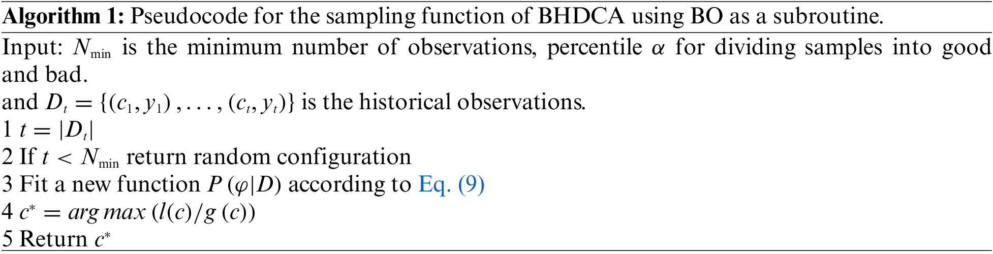
Specifically, the proposed BHDCA utilizes BO to choose the potential parameter configurations. The BO estimates a model to describe the observations’ distribution and samples promising new configurations to refit the model. Meanwhile, hyperband is applied to determine a suitable budget for each configuration to evaluate its performance. The DCA is a part of the evaluation function to measure the performance of parameter configurations. The whole process is cyclical until consuming light the given budget. Fig. 1 illustrates the processes of our proposed BHDCA. The processes of BHDCA contain four steps. Step 1: sample several parameter configurations randomly or based on the function calculated by the BO; step 2: employ the hyperband to allocate a reasonable budget to each parameter configuration; step 3: perform DCA with the given budget and particular parameter configuration to achieve a score of the parameter configuration; step 4: refit a new model by BO to describe these observations’ distribution. The whole process is iterative, looping from step 2 to step 4 until reaching the stop condition. The proposed BHDCA can fully utilize the previous budget to build the model and achieve bright performance.

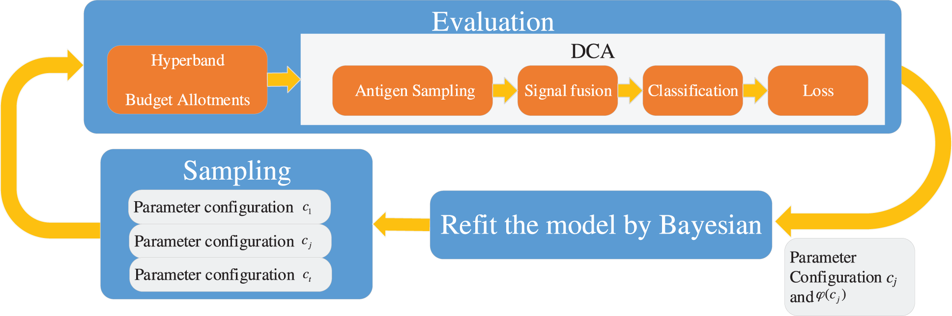
Figure 1: The model of the proposed BHDCA

3.3 BHDCA: Sampling Function

This study transforms parameter optimization into a black-box optimization problem and aims to find the optimal configuration c∗ that maximizes the function φ(cj). Since the given budget B is limited in practice, it’s impossible to perform unlimited optimization work. Therefore, the aim of this study is transformed to find the c+ that maximizes the function φ(cj) with the limited budget B. To explore the observation space D more strategically, this study applies BO to model the relationship between parameter configurations C and φ(C) as a gaussian process regression. The core theory of BO is to predict the posterior data through the prior information constantly. Generally, the distribution function φ(C) of observations is unobservable in DCA. The BO treats it as a random function with a prior over it, samples some observations, updates the prior, refits the model based on those gathering parameter configurations and evaluations, and repeats those processes until reaching an ending condition.

Specifically, this study collects the performance evaluation for each parameter configuration together into a vector [y1,y2,…,yj,…]. The BO assumes that each value in the vector is drawn at random by nature from some prior probability distribution. BO takes this prior distribution to be multi-variate normal with a particular mean vector μ and covariance matrix K. In this study, a functional relationship between the configurations and its performance evaluation accords with the gaussian distribution. The prior distribution of the functional relationship can be considered as the joint distribution of (infinitely many) random variables, as shown in Eq. (7).

P(φ)=G(φ;μ,K)(7)

where the P(φ) is denoted as the probability distribution of the function, G describes the gaussian process regression, the φ is the functional relationship between the parameters and its performance evaluation, the μ is the mean function of φ, the K is the covariance function of the performance evaluations.

The BO assumes that the mapping function φ follows a gaussian distribution, and its conditional distribution also follows a gaussian distribution. Therefore, when the distributions of some observations are known, the function still follows a gaussian distribution as shown in Eq. (8).

P(φ|Dt)=G(φ;μφ|Dt,Kφ|Dt)(8)

where P(φ|Dt) is denoted as the conditional distribution of the function, Dt is a set of known observations, μφ|Dt is the mean function of φ with the known Dt, Kφ|Dt is the covariance function of φ with the known Dt.

To construct the functional relationship more accurately, this study uses the Tree Parzen Estimator (TPE), which uses a kernel density estimator to model the function Eq. (8). The TPE uses a threshold α to divide observations and construct different distributions. In other words, divide the entire observations into two parts: a hyperparameter probability distribution for good grades and a hyperparameter probability distribution for bad grades. Unlike the classical gaussian process, the TPE uses Eq. (9) as the surrogate to express the functional relationship between parameter configurations and its performance evaluations:

P(φ|Dt)={l(c)=P(y<α|c,Dt)g(c)=P(y≥α|c,Dt)(9)

where α is the threshold to divide observations into two parts, l(c) is the prior distribution of the observations with bad grades, g(c) is the prior distribution of the observations with good grades.

BO utilizes an acquisition function based on the model P(φ|Dt) to select the most promising parameter configurations to explore for the next iteration. This study uses a standard acquisition function, expected improvement (EI), to choose the one with the most significant expected progress over the current max φ(c+). In the acquisition function, the selected configuration is based on the following equation:

c∗=argmincEI(max{ε,μφ|Dt(c∗)−y+}|Dt)(10)

where μφ|D(c∗) is the posterior mean of the surrogate G(φ;μφ|D,Kφ|D), y+ is the current max actual value that has been encountered so far, and ε is a real value to express the difference between the posterior mean and the actual value. The acquisition function aims to find the parameter configuration which is greater ε than the current maximum y+. In essence, this study selects the point that minimizes the distance to the current maximum configuration. The ε determines the amount of exploration of the EI acquisition function. The EI function is as follows:

EI(c)=∫max(ε,μφ|Dt(c)−y+)dp(φ|Dt)(11)

According to the work in [37], the max EI in Eq. (11) can be obtained by maximizing the ratio l(c)/g(c). By maximizing the EI function, a promising configuration can be obtained. The whole process of sampling is shown in Algorithm 1.

3.4 BHDCA: Evaluation Function

Exploring configurations is undoubtedly a high cost if each potential configuration is allocated to the whole budget. Due to the expensive resource consumption, this study defines a cheap-to-evaluate approximate value φ~(cj,b), which is the value of φ(cj) with the budget b∈[bmin,bmax], to represent the original φ(cj). With the maximum budget b = bmax, this study denotes that φ~(cj,b)=φ(cj). In essence, performing DCA with specified parameters configuration cj and the budget bmax can obtain the actual value of φ(cj). If b<bmax, the φ(cj,b) is the approximation value of φ(cj), whose quality typically increases with the budget b.

However, for a fixed b, it is not clear a priori whether more configurations (Nsample is large) should be considered with a small average training time, or less configurations (Nsample is small) with longer average training times. In essence, a suitable budget b for performing DCA with promising configuration is crucial for economizing resources and is difficult to determine without a clear prior. The hyperband can address the problem by performing a grid search over the feasible value bmax and employing a principled early-stopping strategy to allocate more resources to more promising parameter configurations. This study uses Hyperband to determine the budget for each parameter configuration and confirms the promising parameter configurations that should be allocated more. The hyperband of BHDCA is shown in Algorithm 2, which maintains two loops: the inner loop and the outer loop. The inner loop follows the way of Successive Halving with a fixed budget. In the inner loop, this study samples promising configurations by bayesian optimization, allocates fewer resources to each parameter configuration, evaluates the objective function values of all configurations, and repeats until reaching the stop condition. By continually cyclic iterative, more resources are concentrated on the observations of follow-up exploration to obtain their objective function values. The outer loop allocates max budget bmax and the max observation number Nsample for each inner loop. This study expects to focus more budgets on more promising configurations. With the bayesian exploration, it will get closer and closer to the globally optimal configuration. Thus, with iteration, the outer loop sets up fewer configurations Nsample to explore and a larger maximum budget bmax used to satisfy φ~(cj,bmax)=φ(cj).

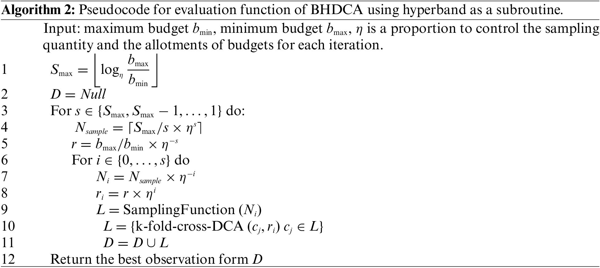
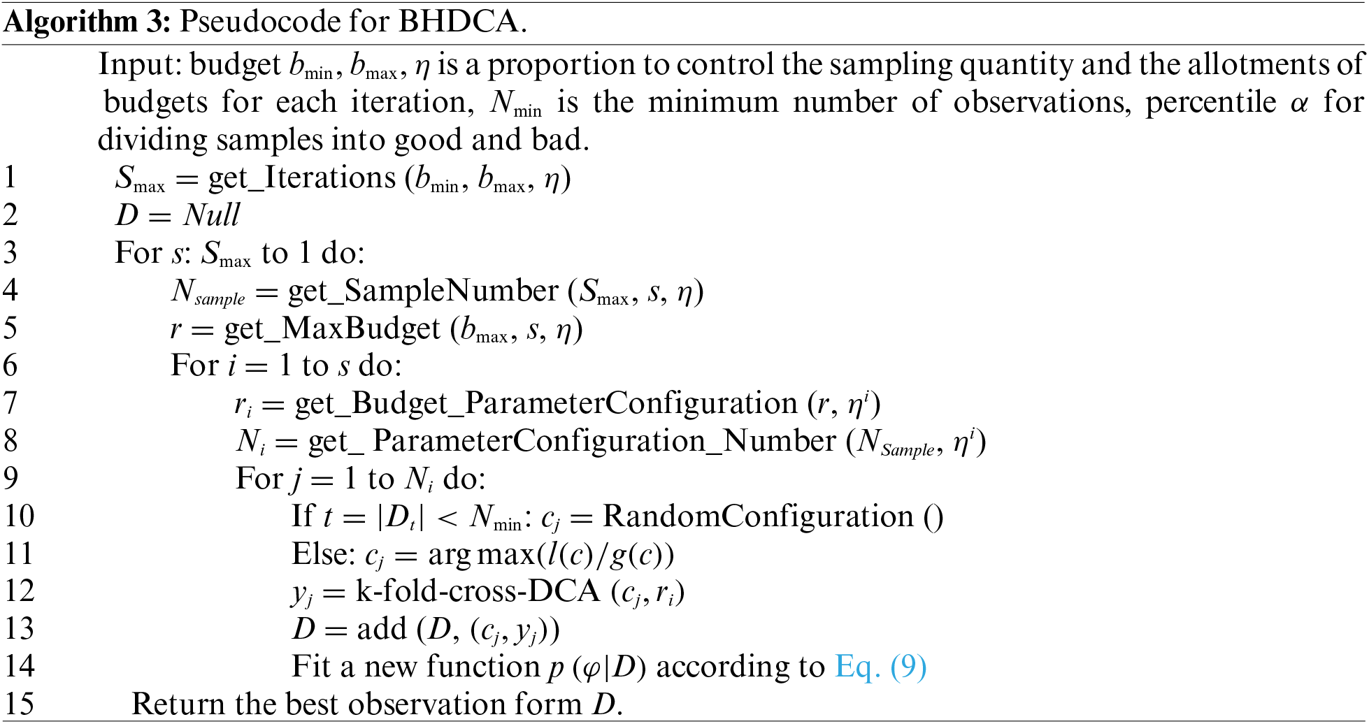
The proposed BHDCA is shown in Algorithm 3, containing two loops: inner and outer. The inner loop is considered a pool of workers, and the outer loop allocates a suitable budget for each pool. In other words, the hyperband maintains a pool of workers and allocates a suitable budget for each pool. Each iteration with a given budget is considered a worker. The BO is used to choose the promising potential configuration for each worker until exhausting all the workers in a pool. The BO treats the objective function as a random function with a prior and utilizes a surrogate in Eq. (9) to model the actual function. Based on the surrogate, the BO can choose the promising potential configurations through an acquisition function. The worker uses the given budget and configuration to calculate its performance evaluation and refits the model based on the new observation. The two processes are iterative until reaching the ending condition.

4  Experimentation

4.1 Data Sets

This study employs the data sets from UCI Machine Learning Repository [35] and Keel-dataset Repository [36] to validate the proposed BHDCA. The description of those data sets is shown in Table 2.

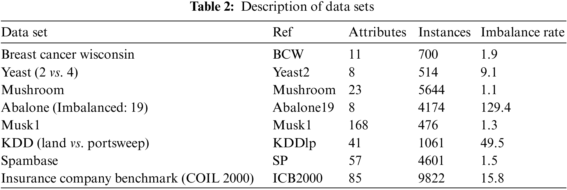
As shown in Table 2, this study organizes three dimensions: feature dimension, data set size, and balance rate. Each dimension contains two data sets. Therefore, this study employs eight different data sets, including a balanced small-sized low-dimensional data set (BCW), an imbalanced small-sized low-dimensional data set (Yeast2), a balanced large-sized low-dimensional data set (Mushroom), an imbalanced large-sized low-dimensional data set (Abalone19), a balanced small-sized high-dimensional data set (Musk1), an imbalanced small-sized high-dimensional data set (KDDlp), a balanced large-sized high-dimensional data set (SP), and an imbalanced large-sized high-dimensional data set (ICB2000). Through performing classification on these data sets, the performance of BHDCA can be thoroughly tested.

In this work, non-numerical features are transformed into numerical parts. Due to the significant effect of singularities on the algorithm, this study utilizes Quartile to find them out. The Quartile uses Eq. (12) to divide the values of each feature into four parts.

{Q1=⌊(n+1)/4⌋Q2=⌊(n+1)/2⌋Q3=⌊3(n+1)/4⌋(12)

Quartile segments any distribution that’s ordered from low to high into four equal parts. Q1 is the value below which 25% of the distribution lies, Q2 is the middle half of a data set, and Q3 is the value below which 75% lies. Eq. (13) is used to find the singularities. If a data point in a feature whose value is less than its Minimum or more significant than its Maximum, it is denoted as a singularity and is replaced with the mean of this feature.

{Minimum=Q1−3(Q3−Q1)Maximum=Q3+3(Q3−Q1)(13)

Before experiments, this study filters the features with a high percentage of missing values and the elements with only one unique value. Reference [38] proposed an “80% rule” suggested retaining a variable with at least 80% nonzero measurement values and removing the other variable with more than 20% missing data. Meanwhile, the data imputation techniques may not work well for data sets with a high rate of missing values. Thus, this study filters those features with more than 20% missing data. For features with less than 20% missing data, this study used the mean value to complete the missing data. Those features with one unique value cannot be helpful for machine learning because of their zero variance. Thus, this study filters out those features which have only one value. Subsequently, Min-Max Normalization is used to scale data into a proportionate range.

za,b=(xa,b−μa)/σb(14)

where xa,b is the value of ath data item in bth attribute, za,b is the normalized value of xa,b that range is from 0 to 1, μb is the mean of the bth feature, σb is the variance of the bth feature.

4.2 Experiment Setup

To study the feasibility and superiority of the proposed approach, this study compares the BHDCA with the other state-of-the-art DCA expansion algorithms for signal fusion: dDCA, FdDCA, GADCA, and IO-dDCA. This study uses 10-fold cross-validation to estimate the performance of algorithms. Each data set is divided into two disjoint parts: training and testing. The accuracy, specificity, precision, recall, F-measure, the area under the curve (AUC), and receiver operating characteristic (ROC) are calculated to evaluate the performance of the above approaches. Generally, the parameter optimization of hyperband and bayesian is time-consuming, contrary to the lightweight running time of DCA. Thus, the time complexity of the above approaches is also analyzed.

In this work, the size of the DC poll is 100, and up to 10 DCs sample each antigen. The migration threshold of DCA is calculated by Eq. (2) with the configuration of the weight values and the max signal values. For classification, this study adopts the proportion of the anomalous items in a data set as the threshold of MCAV. In this study, the budget of BHDCA is the number of data items to build a model, the minimum budget bmin is 1/81 of the training data, and the maximum budget is the total training data. The η is 3 for BHDCA. The antigen sampling mechanism is not the focus of this study. Thus, this study adopts the same antigen sampling mechanism for all the DCA versions. This study utilizes principal component analysis as the antigen sampling mechanism for each data set to map all the attributes into three input signals. The mean of the features assigned to an input signal is calculated as the signal values.

4.3 Results and Analysis

Tables 3–6 show the experimental results of the five algorithms (dDCA, FdDCA, GADCA, IO-dDCA, and BHDCA) on the eight data sets. The mean and standard deviations of the accuracy obtained by the five algorithms are shown in Table 3. Table 4 shows the mean and standard deviations of precision obtained by those five algorithms. Moreover, this study computes the specificity and F-Measure obtained by the five algorithms, and the results are presented in Tables 5 and 6. The number in bold represents the best result among the five algorithms in all the tables.

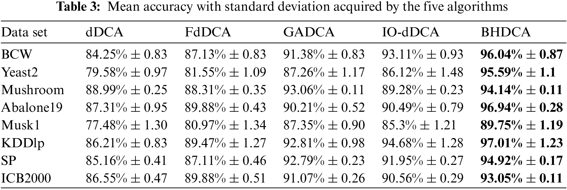
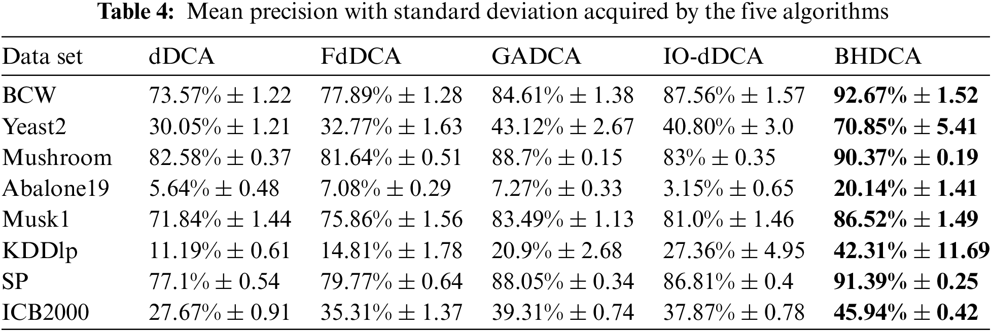
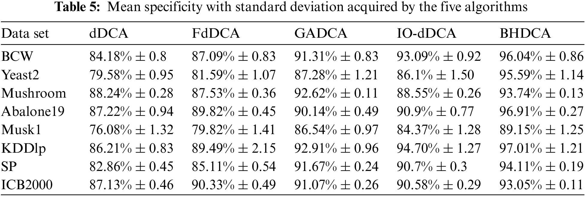
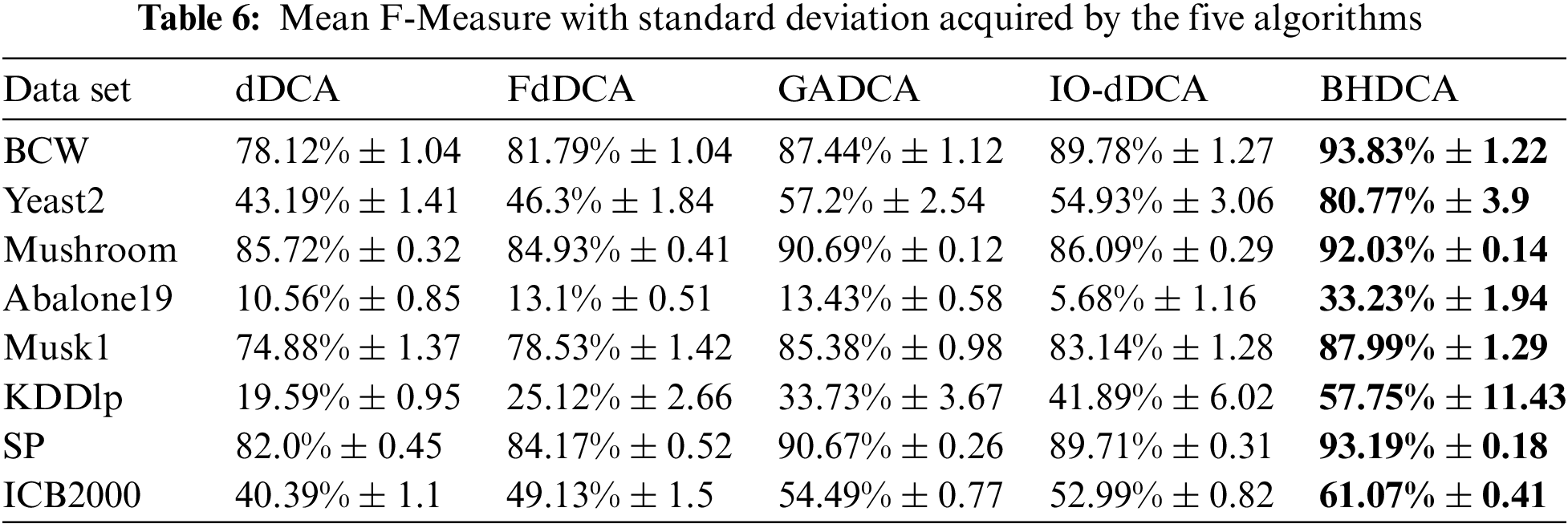
Tables 3–6 show that the proposed BHDCA consistently performs better on the eight data sets than the other DCA versions (e.g., dDCA, FdDCA, GADCA, and IO-dDCA). With the eight data sets, Table 3 illuminates that the difference in accuracy between BHDCA and the other DCA expansion for signal fusion is especially remarkable. For instance, the classification accuracy of BHDCA is at least 2% higher than that of the other DCA versions in the eight data sets. In addition, when the data categories are imbalanced, the precision and F-measure of all algorithms are not ideal, especially on the three data sets: Abalone19, KDDlp, and ICB2000. The reason is that the category ratios of these three data sets are extremely unbalanced (129.4, 49.5, and 15.8, respectively). Table 3 shows that the error rate of the category with a large number of samples is tiny. Still, its total number is large relative to the full sample size of another category due to the unbalanced data sets. Therefore, the precision and F-measure of the DCA versions are not as ideal as the indicator accuracy. However, on the unbalanced data sets, the proposed BHDCA is significantly better than the other DCA versions on the two indicators of precision and F-measure.

To better analyze the results, this study utilizes the t-test to analyze whether significant differences exist in the experiments between the BHDCA and other signal fusion algorithms of DCA (called “Comparisons”) under the condition z = 0.05, as follows:

H0:μBHDCA=μComparisionsH1:μBHDCA≠μComparisions(15)

where H0 is the null hypothesis expressing no significant difference between BHDCA and other DCA expansions in accuracy; H1 is the alternate hypothesis expressing a significant difference between BHDCA and other DCA expansions in accuracy.

The critical t-value is 2.262 when the degree of freedom is nine and the significance level of the t-test is 0.05. Therefore, if the result is below 2.262, hypothesis H0 can be acceptable; otherwise, hypothesis H1 can be acceptable, indicating that significant differences exist. Table 7 shows the t-test results on accuracy and illuminates all the t-value exceeding 2.262. It can be concluded that in terms of classification accuracy, our algorithm BHDCA and the other signal fusion algorithms of DCA exhibit significant differences on all the test problems. The results accordingly prove once again, from a statistical point of view, that our algorithm is the best in all test problems compared with the DCA expansion algorithms.

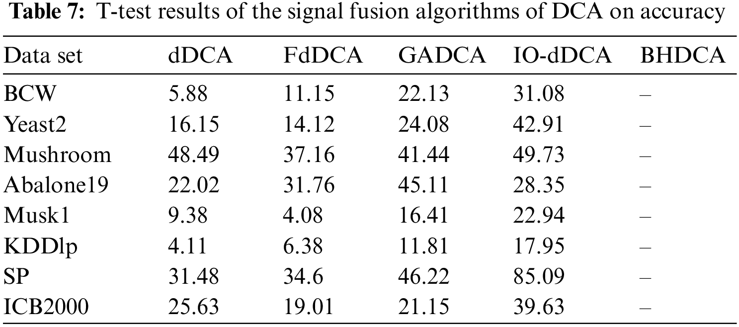
Fig. 2 illustrates that the proposed BHDCA always has a good advantage in terms of AUC. The proposed BHDCA has the most significant AUC with all eight data sets compared to other DCA expansions for signal fusion. Thus, it can be concluded that the proposed BHDCA is superior to the state-of-the-art DCA versions (e.g., dDCA, FdDCA, GADCA, and IO-dDCA) over all the UCI and Keel data sets in a statistically significant manner.

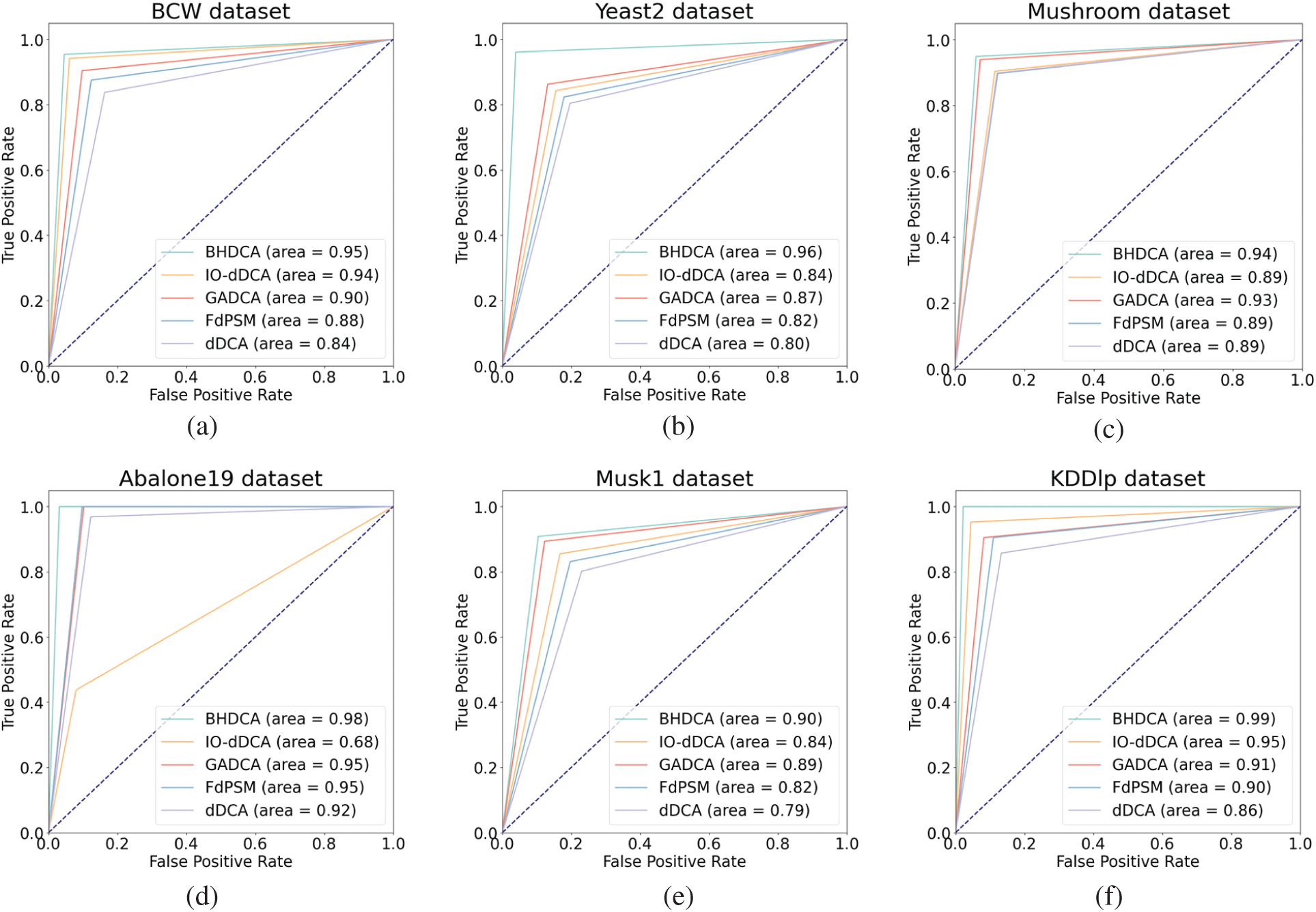
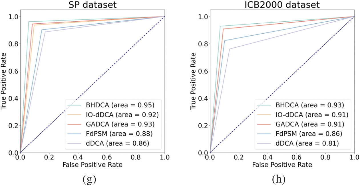
Figure 2: Analysis of the DCA expansions for signal fusion in ROC space

4.4 Complexity Analysis

In this section, the effect of the proposed BHDCA is analyzed in detail about running time. Table 8 shows the detail of all the primitive operations of the BHDCA. In Table 8, each line contains one operation, and the number of times that operation is executed corresponds to Algorithm 3.

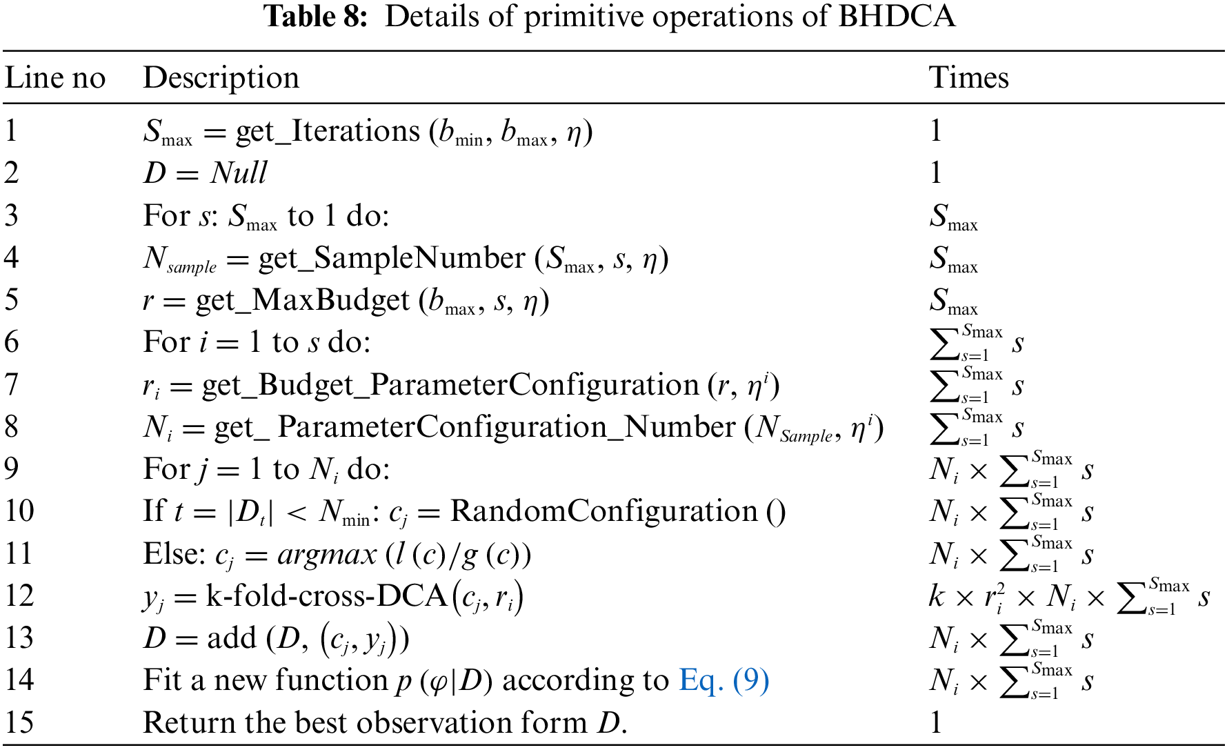
The BHDCA wraps a search task around the DCA. The runtime of BHDCA depends on the iteration number of hyperband, the iteration number of bayesian, and the runtime of DCA. According to work by Gu et al. [39], the runtime complexity of DCA is bounded by O(n2) (n is the data size). Generally, the hyperband and bayesian iteration number depend on the initial budget [bmin, bmax] and the proportion η. Thus, the runtime complexity of the BHDCA is calculated as follows:

T(n)=3+3×Smax+5×∑s=1Smaxs+5×Ni×∑s=1Smaxs+Ni×k×ri2×∑s=1Smaxs(16)

where Ni is the number of the parameter configurations, the max Ni is Nsample, Nsample is the maximum sampling quantity, the maximum Nsample is ⌈Smax×ηSmax⌉, k is set as 5 in this study, ri is the size of the data set for each configuration, the max ri is the data size n. Thus, the runtime is calculated as follows:

T(n)=3×Smax+5×Smax×∑s=1Smaxs+5×Smax×ηSmax×∑s=1Smaxs+k×n2×Smax×ηSmax×∑s=1Smaxs=>Smax+(ηSmax+k×ηSmax×n2)×Smax×∑s=1SmaxsT(n)≈ Smax(Smax+1)2(n2×Smax×ηSmax)≈ n2×Smax3×ηSmax(17)

As shown in Eq. (17), BHDCA has a worse-case runtime complexity of O(n2×Smax3×ηSmax). To further verify the performance of BHDCA, this study calculates the running time of the DCA versions performing classification on the eight datasets. Fig. 3 depicts that the BHDCA maintains the runtime advantage compared with FdDCA, IODCA, and GADCA on most data sets (especially the large-sized high-dimensional data sets). The FdDCA requires an additional Fuzzy c-means algorithm to supersede the original signal fusion, and the Fuzzy c-means algorithm is very time-consuming. Both the GADCA and IO-dDCA require a certain number of iterations to complete parameter optimization. In each of their iterations, they utilize the whole data to evaluate the performance of parameter configurations. However, the BHDCA can allocate suitable data for each configuration, not the entire data. Therefore, the BHDCA needs less runtime than GADCA and IO-dDCA with the same iterations. Although dDCA requires less running time, the reason is that it only involves experience to set the parameters without the training phase. However, it’s undesired and does not produce stable results. Compared with dDCA, BHDCA can automatically adjust the parameters according to the application field and adapt to a broader range of application fields. Thus, in light of the performance improvement offered by the BHDCA, our algorithm BHDCA is the best in all test problems.

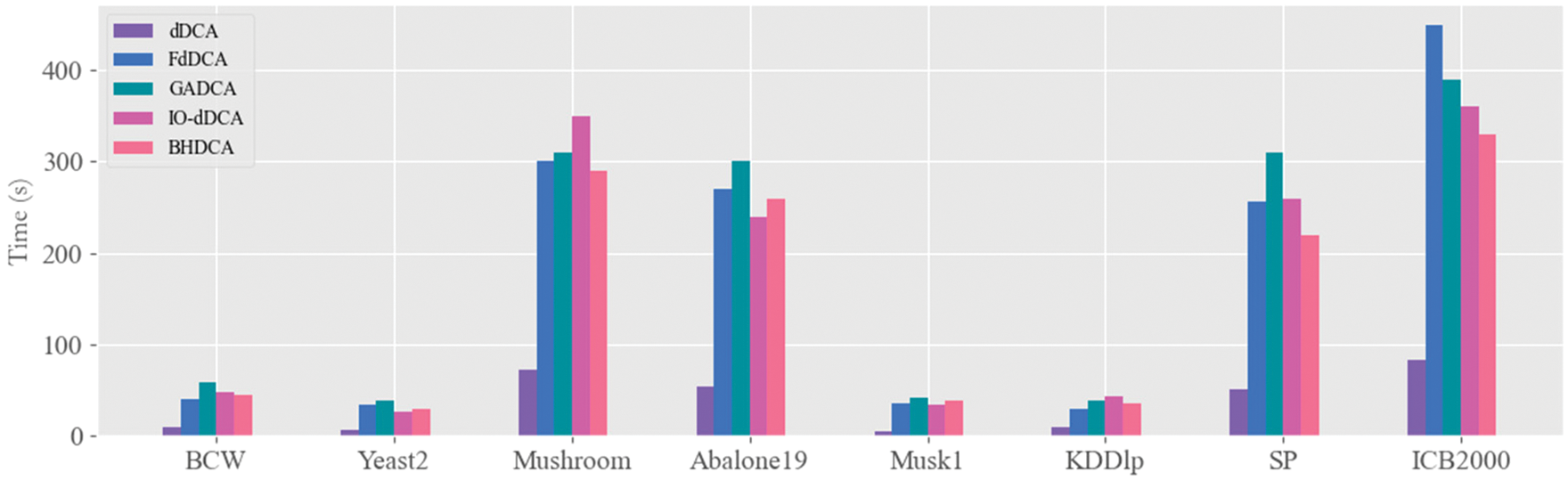
Figure 3: Mean execution time (in seconds) acquired by DCA versions

5  Conclusion

Due to a poor understanding of the underlying classification mechanism, optimizing the objective function φ is complex. Therefore, this study models the work of parameter optimization into a black-box problem. By analyzing the DCA procedure, this study confirms all the parameters to be optimized in signal fusion. To discover the optimal parameter configuration, the BOHB is applied to model the distribution of observations to sample promising configurations and then allocate a reasonable budget for each chosen configuration. A novel DCA expansion algorithm, BHDCA, is proposed to automatically perform parameter optimization in DCA without any information about the loss function, which hybrids DCA and BOHB. The proposed BHDCA applies BO to explore the searching space with all potential parameter configurations and chooses the promising configurations to allot a reasonable budget by hyperband. To verify the performance of BHDCA, this study implemented two parts of experiments. In the first part, the proposed BHDCA is compared with the state-of-the-art DCA expansion algorithms for signal fusion (e.g., dDCA, FdDCA, GADCA, and IO-dDCA). The classification results indicate that BHDCA is superior to other DCA-derived classification algorithms on all test problems. The other part discusses the runtime of these DCA versions (e.g., dDCA, FdDCA, GADCA, IO-dDCA, and BHDCA). This study analysis the time complexity of BHDCA and compares the runtime of all the DCA versions on each data set. The experimental results show that the proposed BHDCA maintains its advantage on most tests (especially the large-sized high-dimensional data sets) regarding runtime. The findings reported here shed new light on two parts. Firstly, model the parameter configures and their corresponding performance as a gaussian process and utilize BO to construct a surrogate to express the functional relationship for exploring the observations. Secondly, apply hyperband to allocate a suitable budget for each selected observation. The BHDCA can ignore the unnecessary parameter configuration and allocate a suitable budget instead of the entire dataset. The finding will be of interest to optimize the parameters of DCA without any domain expertise for extending more domains; reduce the training time of DCA for scaling evolution up to large-scale data sets.

Since the steps of the algorithm are run serially, a limitation of this study is that the calculation time could be more optimistic. To evaluate the parameter configurations, this study performs the classification of DCA many times in each iteration of the hyperband, and each evaluation is independent of the other. These works run serially and consume the most runtime of BHDCA. For future work, employing a parallel strategy to run BHDCA is the next step to reduce the runtime better. The DCA classification in each hyperband iteration will run concurrently to reduce runtime. In addition, hybridizing the heuristic algorithms (i.e., elephant herding optimization (EHO) [40], moth search (MS) algorithm [41], and particle-swarm krill herd (PKH) [42]) and hyperband algorithm is also our next research direction. Combining the heuristic algorithm’s convergence ability with the hyperband’s dynamic resource allocation can reduce resource consumption.

Funding Statement: The author (Y. Liang) received National Natural Science Foundation of China with the Grant Number 61877045 for this study http://www.nsfc.gov.cn/.

Conflicts of Interest: The authors declare that they have no conflicts of interest to report regarding the present study.

References

1. Z. Wen and Y. Liang, “A new version of the deterministic dendritic cell algorithm based on numerical differential and immune response,” Applied Soft Computing, vol. 102, no. 107055, pp. 161–173, 2021. [Google Scholar]

2. J. Greensmith and U. Aickelin, “The deterministic dendritic cell algorithm,” in Int. Conf. on Artificial Immune Systems (ICARS), Phuket, Thailand, pp. 291–302, 2008. [Google Scholar]

3. Z. C. Dagdia, “A scalable and distributed dendritic cell algorithm for big data classification,” Swarm and Evolutionary Computation, vol. 50, no. 100432, pp. 89–101, 2019. [Google Scholar]

4. C. Zhang and Z. Yi, “A danger theory inspired artificial immune algorithm for on-line supervised two-class classification problem,” Neurocomputing, vol. 73, no. 7, pp. 1244–1255, 2010. [Google Scholar]

5. M. Abdelhaq, R. Hassan and R. Alsaqour, “Using dendritic cell algorithm to detect the resource consumption attack over MANET,” in Software Engineering and Computer Systems (ICSECS). Heidelberg, Berlin, Germany: Springer, pp. 429–442, 2011. [Google Scholar]

6. E. Farzadnia, H. Shirazi and A. Nowroozi, “A novel sophisticated hybrid method for intrusion detection using the artificial immune system,” Journal of Information Security and Applications, vol. 70, no. 102721, pp. 2214–2126, 2022. [Google Scholar]

7. D. Limon-Cantu and V. Alarcon-Aquino, “Multiresolution dendritic cell algorithm for network anomaly detection,” PeerJ Computer Science, vol. 7, no. 8, 749, 2021. [Google Scholar]

8. C. Duru, J. Ladeji-Osias, K. Wandji, T. Otily and R. Kone, “A review of human immune inspired algorithms for intrusion detection systems,” in 2022 IEEE World AI IoT Congress (AIIoT). Seattle, WA, USA, pp. 364–371, 2022. [Google Scholar]

9. E. -S. M. El-Alfy and A. A. Al-Hasan, “A novel bio-inspired predictive model for spam filtering based on dendritic cell algorithm,” in IEEE Symp. on Computational Intelligence in Cyber Security (CICS), Orlando, Florida, U.S.A, pp. 1–7, 2014. [Google Scholar]

10. W. Chen, H. Zhao, T. Li and Y. Liu, “Optimal probabilistic encryption for distributed detection in wireless sensor networks based on immune differential evolution algorithm,” Wireless Networks, vol. 24, no. 7, pp. 2497–2507, 2018. [Google Scholar]

11. W. Zhou, Y. Liang, Z. Ming and H. Dong, “Earthquake prediction model based on danger theory in artificial immunity,” Neural Network World, vol. 30, no. 4, pp. 231–247, 2020. [Google Scholar]

12. J. Greensmith and L. Yang, “Two DCA: A 2-dimensional dendritic cell algorithm with dynamic cell migration,” in 2022 IEEE Congress on Evolutionary Computation (CEC), Padua, Italy, pp. 1–8, 2022. [Google Scholar]

13. B. Bejoy, G. Raju, D. Swain, B. Acharya and Y. Hu, “A generic cyber immune framework for anomaly detection using artificial immune systems,” Applied Soft Computing, vol. 130, no. 10, 109680, 2022. [Google Scholar]

14. O. Igbe, I. Darwish and T. Saadawi, “Deterministic dendritic cell algorithm application to smart grid cyber-attack detection,” in 2017 IEEE 4th Int. Conf. on Cyber Security and Cloud Computing (CSCloud), New York, NY, USA, pp. 199–204, 2017. [Google Scholar]

15. A. Diez-Olivan, P. Ortego, J. Del Ser, I. Landa-Torres, D. Galar et al., “Adaptive dendritic cell-deep learning approach for industrial prognosis under changing conditions,” IEEE Transactions on Industrial Informatics, vol. 17, no. 11, pp. 7760–7770, 2021. [Google Scholar]

16. Z. Chelly and Z. Elouedi, “A survey of the dendritic cell algorithm,” Knowledge and Information Systems, vol. 48, no. 3, pp. 505–535, 2016. [Google Scholar]

17. J. Greensmith and U. Aickelin, “The deterministic dendritic cell algorithm,” in Int. Conf. on Artificial Immune Systems (ICARIS), Phuket, Thailand, pp. 291–302, 2008. [Google Scholar]

18. J. Greensmith and M. B. Gale, “The functional dendritic cell algorithm: A formal specification with haskell,” in IEEE Congress on Evolutionary Computation (CEC), Donostia-San Sebastian, Spain, pp. 1787–1794, 2017. [Google Scholar]

19. N. Mukhtar, G. M. Coghill and W. Pang, “FdDCA: A novel fuzzy deterministic dendritic cell algorithm,” in Genetic and Evolutionary Computation Conf. Companion (GECCO), New York, NY, USA, pp. 1007–1010, 2016. [Google Scholar]

20. C. J. Musselle, “Insights into the antigen sampling component of the dendritic cell algorithm,” in Int. Conf. on Artificial Immune Systems (ICARIS), Edinburgh, UK, pp. 88–101, 2010. [Google Scholar]

21. J. Greensmith, “Migration threshold tuning in the deterministic dendritic dell algorithm,” in Theory and Practice of Natural Computing (TPNC). Kingston, Canada, Cham: Springer, pp. 122–133, 2019. [Google Scholar]

22. T. Stibor, R. Oates, G. Kendall and J. M. Garibaldi, “Geometrical insights into the dendritic cell algorithm,” in Genetic and Evolutionary Computation (GECCO). New York, USA: Association for Computing Machinery, pp. 1275–1282, 2009. [Google Scholar]

23. W. Zhou and Y. Liang, “An immune optimization based deterministic dendritic cell algorithm,” Applied Intelligence, vol. 52, no. 2, pp. 1461–1476, 2022. [Google Scholar]

24. N. Elisa, L. Yang and F. Chao, “Signal categorization for dendritic cell algorithm using GA with partial shuffle mutation,” in UK Workshop on Computational Intelligence (UKCI). Portsmouth, UK, pp. 529–540, 2019. [Google Scholar]

25. S. Falkner, A. Klein and F. Hutter, “BOHB: Robust and efficient hyperparameter optimization at scale,” in Int. Conf. on Machine Learning (ICML), Stockholm, Sweden, pp. 1437–1446, 2018. [Google Scholar]

26. J. Bergstra and Y. Bengio, “Random search for hyper-parameter optimization,” Journal of Machine Learning Research, vol. 13, no. 10, pp. 281–305, 2012. [Google Scholar]

27. J. Verwaeren, P. Van der Weeen and B. De Baets, “A search grid for parameter optimization as a byproduct of model sensitivity analysis,” Applied Mathematics and Computation, vol. 261, no. 3, pp. 8–27, 2015. [Google Scholar]

28. J. Nalepa and P. R. Lorenzo, “Convergence analysis of PSO for hyper-parameter selection in deep neural networks,” in Int. Conf. on P2P, Parallel, Grid, Cloud and Internet Computing (3PGCIC), Barcelona, SPAIN, pp. 284–295, 2017. [Google Scholar]

29. A. H. Victoria and G. Maragatham, “Automatic tuning of hyperparameters using bayesian optimization,” Evolving Systems, vol. 12, no. 1, pp. 217–223, 2021. [Google Scholar]

30. K. Kandasamy, G. Dasarathy, J. Oliva, J. Schneider and B. Poczos, “Gaussian process bandit optimization with multi-fidelity evaluations,” in Int. Conf. on Neural Information Processing Systems (NIPS), New York, NY, USA, pp. 1000–1008, 2016. [Google Scholar]

31. K. Kandasamy, G. Dasarathy, J. Oliva, J. Schneider and B. Poczos, “Multi-fidelity bayesian optimisation with continuous approximations,” in Int. Machine Learning Society (IMLS). Sydney, Australia, pp. 2861–2878, 2017. [Google Scholar]

32. G. G. Wang, D. Gao and W. Pedrycz, “Solving multiobjective fuzzy job-shop scheduling problem by a hybrid adaptive differential evolution algorithm,” IEEE Transactions on Industrial Informatics, vol. 18, no. 12, pp. 8519–8528, 2022. [Google Scholar]

33. D. Gao, G. G. Wang and W. Pedrycz, “Solving fuzzy job-shop scheduling problem using DE algorithm improved by a selection mechanism,” IEEE Transactions on Fuzzy Systems, vol. 28, no. 12, pp. 3265–3275, 2020. [Google Scholar]

34. L. Li, K. Jamieson, G. DeSalvo, A. Rostamizadeh and A. Talwalkar, “Hyperband: A novel bandit-based approach to hyperparameter optimization,” The Journal of Machine Learning Research, vol. 18, no. 185, pp. 6765–6816, 2017. [Google Scholar]

35. A. Asuncion and D. Newman, UCI Machine Learning Repository. Irvine, California, UAS: University of California, School of Information and Computer Science, 2007. [Google Scholar]

36. I. Triguero, S. González, J. M. Moyano, S. García, J. Alcala-Fdez et al., “KEEL 3.0: An open-source software for multi-stage analysis in data mining,” International Journal of Computational Intelligence Systems, vol. 10, no. 1, pp. 1238–1249, 2017. [Google Scholar]

37. J. Bergstra, R. Bardenet, Y. Bengio and B. Kegl, “Algorithms for hyper-parameter optimization,” in Int. Conf. on Neural Information Processing Systems (NIPS), New York, NY, USA, pp. 2546–2554, 2011. [Google Scholar]

38. S. Bijlsma, I. Bobeldijk, E. R. Verheij, R. Ramaker, S. Kochhar et al., “Large-scale human metabolomics studies: A strategy for data (pre-) processing and validation,” Analytical Chemistry, vol. 78, no. 2, pp. 567–574, 2006. [Google Scholar] [PubMed]

39. F. Gu, J. Greensmith and U. Aickelin, “Theoretical formulation and analysis of the deterministic dendritic cell algorithm,” Biosystems, vol. 111, no. 2, pp. 127–135, 2013. [Google Scholar] [PubMed]

40. G. G. Wang, S. Deb and L. D. S. Coelho, “Elephant herding optimization,” in Int. Symp. on Computational and Business Intelligence (ISCBI), Bali, Indonesia, pp. 1–5, 2015. [Google Scholar]

41. G. G. Wang, “Moth search algorithm: A bio-inspired metaheuristic algorithm for global optimization problems,” Memetic Computing, vol. 10, no. 3, pp. 151–164, 2018. [Google Scholar]

42. G. G. Wang, D. Bai, W. Gong, T. Ren, X. Liu et al., “Particle-swarm krill herd algorithm,” in 2018 IEEE Int. Conf. on Industrial Engineering and Engineering Management (IEEM), Bangkok, Thailand, pp. 1073–1080, 2018. [Google Scholar]