Multi-Attribute Couplings-Based Euclidean and Nominal Distances for Unlabeled Nominal Data

1  Introduction

Unlabeled nominal data is widely seen in real-world data and applications. Table 1 illustrates an unlabeled nominal data set with six objects (six students), a fragment of the Student Performance data in the UCI Machine Learning Repository. The attributes Mjob, Fjob, and Reason are nominal, respectively, describing “mother’s job”, “father’s job” and “reason to choose this school”, and all the attribute values of this data set are nominal. Typical data characteristics in nominal attributes include: (1) the values of a nominal attribute do not necessarily have a numeric order. Hence they are not numerically comparable [1]; (2) attributes are more or less coupled with each other w.r.t. various aspects or reasons, e.g., similar frequencies of two values, the co-occurrences of values of two-to-many attributes on the same objects. These form various couplings related to attributes [2] and a significant challenge of learning from non-IID data [3], which has attracted recent interest in machine learning and data mining of nominal data. For example, in Table 1, the attribute Reason has four values: ‘course’ (course preference), ‘reputation’ (school reputation), ‘home’ (close to home), and ‘other’ (other reasons). To deeply understand why a student chooses a school, this paper has to explore (1) the reason which explicitly explains the driving factor and (2) the implicit couplings between attributes, e.g., why a student chooses a school may also be affected by the student’s gender and mother/father’s job situations, especially when the reasons may not be informative or determinate enough. Further, if this paper wants to measure the decision-making dissimilarity (or similarity) between students in choosing schools, it is clear that this paper has to not only measure the value dissimilarity within each attribute but also quantify the different effects of the attribute.

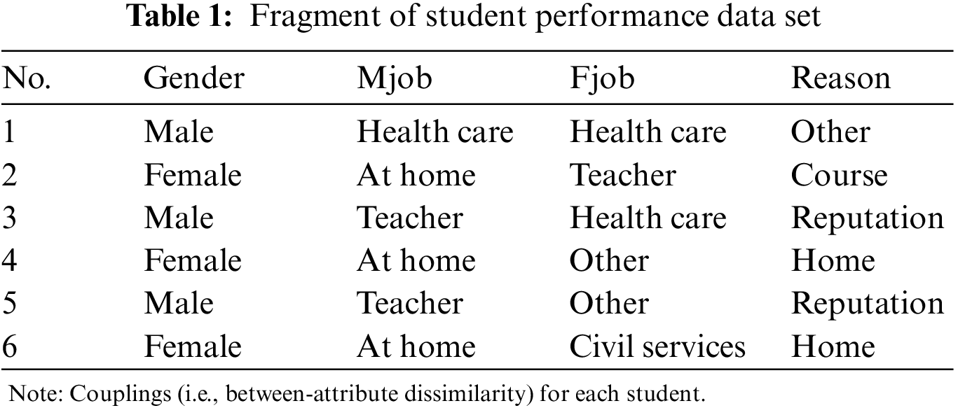
Much less research, theories, and tools are available for handling nominal data in comparison with numerical data. Unlabeled nominal data analysis needs to quantify the similarity (or distance) between objects described by nominal attributes. Numerical distance measures such as the Euclidean distance cannot be applied to such data, and the existing similarity and measures for categorical data also cannot effectively represent the attribute coupling relationships in nominal data. This is the reason that nominal data cannot be handled by numerical data-oriented similarity measures and computing methods. In general, the distance measures for nominal data can be categorized into two: one is to design specific Nominal Distance Measures called NDM for nominal data, and the other is to convert nominal data to numeric and then apply the Euclidean Distance Metric (EDM). There are different NDM measures designed to measure the dissimilarity between two values of an attribute, e.g., the basic Hamming distance (HAM_NDM) [4], the distance metric based on rough membership function (RMF_NDM) [5], the HongJia’s distance metric (HJM_NDM) [6], and the coupled distance metric (CMS_NDM) [7]. However, NDM is typically incorporated into a special nominal clustering algorithm, e.g., K-modes [8], and thus the use of NDM is often restricted. EDM measures require the nominal-to-numeric data conversion, with usual transformation methods such as based on the dummy variables (DV_EDM) [9], related to the inverse document frequency (IDF_EDM) [10], and by modeling hierarchical value couplings (CDE_EDM) [11]. Nevertheless, there are few methods to transform nominal data to numeric for applying EDM, and the transformation has to capture the underlying data characteristics in nominal data that are different from that of numeric data.

This paper proposes a novel and effective distance called the Multi-attribute Couplings-based Distances (MCD) to learn the distance between nominal objects by involving the multi-dimensional couplings between many attributes. There are three features in MCD. First, MCD captures multi-attribute couplings, i.e., the interactions between two nominal attributes, three nominal attributes, four nominal attributes, etc. Second, MCD quantifies the essential characteristics of attribute values in both the raw data set and newly constructed data set based on multi-attribute couplings by the self-information and the related attribute entropy. Lastly, MCD measures the strengths of multi-attribute couplings in terms of the value’s essential characteristics in raw and newly constructed data sets and normalizes the strengths to build the distance metric for nominal data. Taking Table 1 as an example, RMF _NDM treats the value of attribute Fjob on the 3rd student utterly the same as that of the 4th student because two values ‘health care’ and ‘other’ have the same frequency on all students in this data set. HJM_NDM and CDE_EDM instead believe the 1st and 3rd students share strong similarity since the values of two attributes Gender and Fjob for these two students are equivalent. CMS_NDM considers that there may be possible relations between the two values (‘at home’ and ‘teacher’) of attribute Mjob for the 4th and 5th students because two values (‘other’) of attribute Fjob for these two students are identical. These distance measures capture attribute couplings that only can present pairwise value-value relations either within an attribute or between two attributes, but they overlook multi-dimensional attribute couplings (or multi-attribute couplings). MCD is distinct from them. It can not only measure the similarity between the 2nd, 4th, and 6th students in terms of the pairwise value relations between two general attributes Gender and Mjob but also disclose the difference between the 2nd and 4th students and the 4th and 6th students in terms of the interactions between three general attributes Gender, Mjob and Reason (i.e., three-attribute coupling). These interactions form a new attribute {Gender, Mjob, Reason}, where the 2nd and 4th students share different new values, i.e., {‘female’, ‘at home’, ‘course’} and {‘female’, ‘at home’, ‘home’} while the 4th and 6th students share the same new value {‘female’, ‘at home’, ‘home’}. This example shows that MCD can disclose deep multi-dimensional coupling relationships between attributes for deeper object similarity measurement. Moreover, different from existing distance metrics which either take the NDM or the EDM direction, MCD produces both NDM and EDM-oriented distance metrics, called MC_NDM and MC_EDM. They can be individually incorporated into numerical or specific nominal clustering methods, such as K-means and K-modes, hence, significantly improving the flexibility of nominal data clustering, and many numeric clustering methods can be directly applied to nominal data.

The rest of this paper is organized as follows. In Section 2, this research briefly reviews the existing distance measures for unlabeled nominal data. The preliminary explanations and definitions are specified in Section 3, Section 4 introduces the multi-attribute couplings-based distance MCD, and Section 5 shows the experimental results on 15 nominal data sets. Lastly, the conclusion is drawn in Section 6.

2  Related Work

In this section, this paper reviews the distance measures for nominal data, covering those either not involving value relations within and between attributes or building on the principle of coupling learning. Coupling learning is a general learning framework to mainly obtain value relations and attribute couplings and then build the similarity of objects [2]. Couplings generally refer to any relationships and interactions between values and between attributes. Coupling learning has been successfully applied to various learning tasks and data applications, such as similarity and metric learning of categorical [12], numerical [13], and mixed data [14]; outlier detection for high-dimensional, redundant, and noisy data [15]; document analysis [16]; high-dimensional financial data analysis [17]; and individual and group behavior analysis [18].

Here, this paper focuses on coupling-based distance learning and categorizes the related work into four classes. The first class includes distance measures without considering any value and attribute relations. DV_EDM and IDF_EDM fall into this class. DV_EDM [9] converts a nominal value to an integer number and treats a nominal attribute value as a dummy variable with a truth value represented by 0 or 1. IDF_EDM originated from the inverse document frequency (IDF) applied to word counting in documents for tasks such as information extraction, text categorization, and topic modeling [10]. To make IDF applicable for nominal data, this paper can treat each nominal attribute as a unique document collected in a corpus and consider each different value of an attribute as a ‘term’, and then the IDF is calculated on the values of each attribute. IDF_EDM thus measures value similarity w.r.t. the occurrence frequency of a value of a nominal attribute. The IDF can be regarded as the attribute value self-information [19] in IDF_EDM. The second class refers to distance measures by considering the relationships between two values from the same nominal attribute, i.e., intra-attribute value relations. HAM_NDM is the most commonly used representative of this class [4]. In HAM_NDM, the dissimilarity degree of two attribute values is set at 0 if two values are identical; otherwise 1. HAM_NDM between two nominal objects equals the number of their mismatched attribute values. Other similarity measures for nominal data similar to HAM_NDM are the Gower similarity, Eskin similarity, and Goodall similarity [20]. RMF_NDM [5] also falls into this category, which regards that two objects share an indistinguishable relation if they have the same value of a nominal attribute. Based on this idea, RMF_NDM incorporates a rough membership function for nominal data. The third class includes the distance measures that learn the relationships between two nominal values of an attribute concerning or conditional on another attribute. Such distance measures are Ahmad’s distance metric [21], the association-based distance metric [22], and the context-based distance metric [23]. However, these neglect the dissimilarity between two values from the same attribute, i.e., intra-attribute value relations. CMSNDM also addresses this issue by defining the intra-attribute value similarity between two values of an attribute and measuring the similarity between two values of an attribute w.r.t. all other attributes as the inter-attribute value similarity and then integrating these two similarities into a decreasing function to form the CMS_NDM distance metric [7]. CMS_NDM follows the idea of building attribute value dissimilarity by modeling intra- and inter-attribute value relations as in [24,25]. The four class consists of distance measures that capture the relationships between two nominal values separately from two different attributes. HJM_NDM [6] and CDE_EDM [11] are representatives of this class. HJM_NDM captures the co-occurrence times of two values from two different attributes selected by the mutual information. CDE_EDM involves not only value relations but also value-cluster relations. CDE_EDM adds all values from all attributes to a value set, constructs the value influence matrices with different value relation functions, and learns the value clusters with different granularities according to the value influence matrices. It further learns the relationships between value clusters and then produces the final value embedding matrices [11]. In CDE_EDM, the value influence matrices are constructed mainly using the co-occurrence frequency of two nominal values from two different attributes.

Unlike the above categories of distance measures, this work explores the multi-attribute couplings and then constructs distance metrics for unlabeled nominal objects. The existing distance measures involve pairwise value relations w.r.t. one to two attributes; however, our proposed MCD explicitly captures the interactions between two to multiple attributes, reflecting multiple dimensional relationships between attribute values in nominal data.

3  Preliminaries

To clearly describe multi-attribute couplings and differentiate them from the existing conceptual systems for nominal data, before this research discusses the proposed multi-attribute couplings-based distance metrics, this paper gives the definitions of a single-value nominal attribute, the multi-attribute coupling and a multi-value nominal attribute.

Definition 1. [Single-value nominal Attribute (SA)] If an attribute is nominal and there is only one value of the nominal attribute for each data object, this attribute is called a single-value nominal attribute.

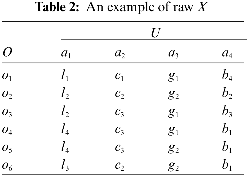
Definition 2. [Multi-attribute coupling] A multi-attribute coupling refers to an interaction between multiple SA decomposed into two-attribute couplings where two SA are coupled with each other, three-attribute couplings where three SA are coupled, ···, or (D−1)-attribute couplings for D-1 coupled SA. For example, as shown in Table 2, there are six objects, i.e., o1 to o6, and four SA, i.e., a1 to a4, and only one nominal value from each SA is assigned to an object. Two SA a1 and a2 in Table 2 may be coupled with each other, forming two-attribute couplings, i.e., C1 = C(a1, a2) is a two-attribute coupling between two SA a1 and a2 w.r.t. the attribute interaction function C also regarded as the coupling function. Similarly, other different two-attribute couplings are obtained such as C2 and C3, and three-attribute coupling C4 for the coupling: C4 = C(a1, a2, a4) between three SA a1, a2 and a4. Table 3 illustrates the multi-attribute couplings.

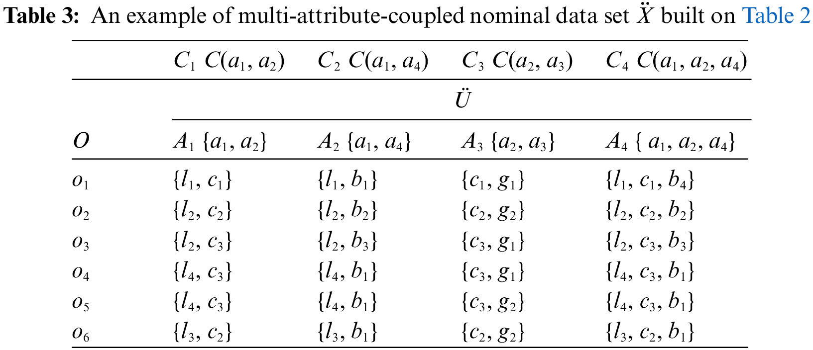
Definition 3. [Multi-value nominal Attribute (MA)] A multi-attribute coupling connects multiple values from the respective SA. A simple way of forming a multi-attribute coupling is to combine the values of the respective SA on each object, and the resultant value combination forms a new attribute. This new attribute is called a multi-value nominal attribute. Subsequently, 2-value nominal attributes, 3-value attributes and (D−1)-value attributes are obtained. For example, in Table 3, built on Table 2, because of the interactions between two SA, two-attribute couplings C1, C2 and C3 lead to the combinations of two SA values and then form three new MA respectively, i.e., 2-value attributes A1, A2 and A3. Similarly, according to three-attribute coupling C4, a new MA is obtained, i.e., 3-value attribute A4. At last, in Table 3, the values of each object are updated in terms of these newly generated 2 to 3-value attributes, e.g., the value of A4 on object o5 is {l4, c3, b1}.

With the above essential concepts, let us further formalize the notations used in this work. Assume a nominal data set X consists of N objects O, O = {o1, o2, ..., oN} and a set U of D SA, i.e., U = {a1, a2, ..., aD}, and vdn is the value of SA ad for the object on. X is a raw data set and can be expressed as a basic information table, such as Table 2. By exploring the multi-attribute couplings, the data set X is converted to a multi-attribute-coupled representation, i.e., a new multi-attribute-coupled data set X¨. where each data object on is represented in terms of a MA set U¨, U¨ = {A1, A2, …, AM}, and each Am newly derived MA corresponds to a multi-attribute coupling Cm. In this new representation X¨, Vmn refers to the value of Am newly derived MA for object on, which is a result of a multi-attribute coupling Cm for the object on. Similarly, this X¨ can be expressed as a multi-attribute-coupled information table, such as Table 3. Here, n∈{1, 2, …, N}, d∈{1, 2, …, D} and m∈{1, 2, …, M}.

For example, Table 2 is the raw nominal data set consisting of six objects and four SA, where v45 = b1 corresponding to the value b1 for object o5 on SA a4; Table 3 is a multi-attribute-coupled representation derived from Table 2 and consists of 2-value attributes {a1, a2}, {a1, a4} and {a2, a3} and 3-value attribute {a1, a2, a4}, and V45 = {l4, c3, b1} is the new value of the A4 = {a1, a2, a4} newly derived MA for object o5. By comparing the values v45 in the raw data set and the new value V45 in the new representation on object o5, Table 3 captures multi-attribute couplings hidden in Table 2.

4  Multi-Attribute-Coupled Distances

This section introduces the algorithm and its working process and constituents for calculating the numerical and nominal multi-attribute couplings-based distances (MCD) between two nominal objects according to multi-attribute couplings.

4.1 The MCD Metric

For two objects oi and oj in the derived multi-attribute-coupled representation (i.e., new X¨) from the raw data set X, our goal is to design distance metrics that can capture the various multi-attribute couplings. Two MCD metrics are defined below on the nominal data set X¨:

E(oi,oj)=‖e→i−e→j‖2(1)

and

S(oi,oj)=∑m=1M⁡|Ψ^(Cm,i)−Ψ^(Cm,j)|(2)

where e→i and e→j are two numerical vectors for oi and oj respectively, e→i is formed by concatenating all strength Ψ^(Cm, i) on all M multi-attribute couplings, and e→j is built on concatenating all Ψ^(Cm, j) (i,j∈{1, 2, ..., N} and m = 1, 2, ..., M). Ψ^(·) is defined in Eq. (9), referring to the normalized strength of a multi-attribute coupling for one object in data set X¨. || · ||2 is the L2 norm and | · | is the operator for obtaining the absolute value.

Subsequently, two MCD metrics defined in Eqs. (1) and (2) refer to a Euclidean distance and a specific nominal distance for nominal data, denoted as MC_EDM and MC_NDM for the consistency and comparison with other related work respectively. MC_EDM and MC_NDM are wanted to enable specific nominal clustering algorithms and numerical clustering algorithms to be respectively applied to the derived data set X¨ directly.

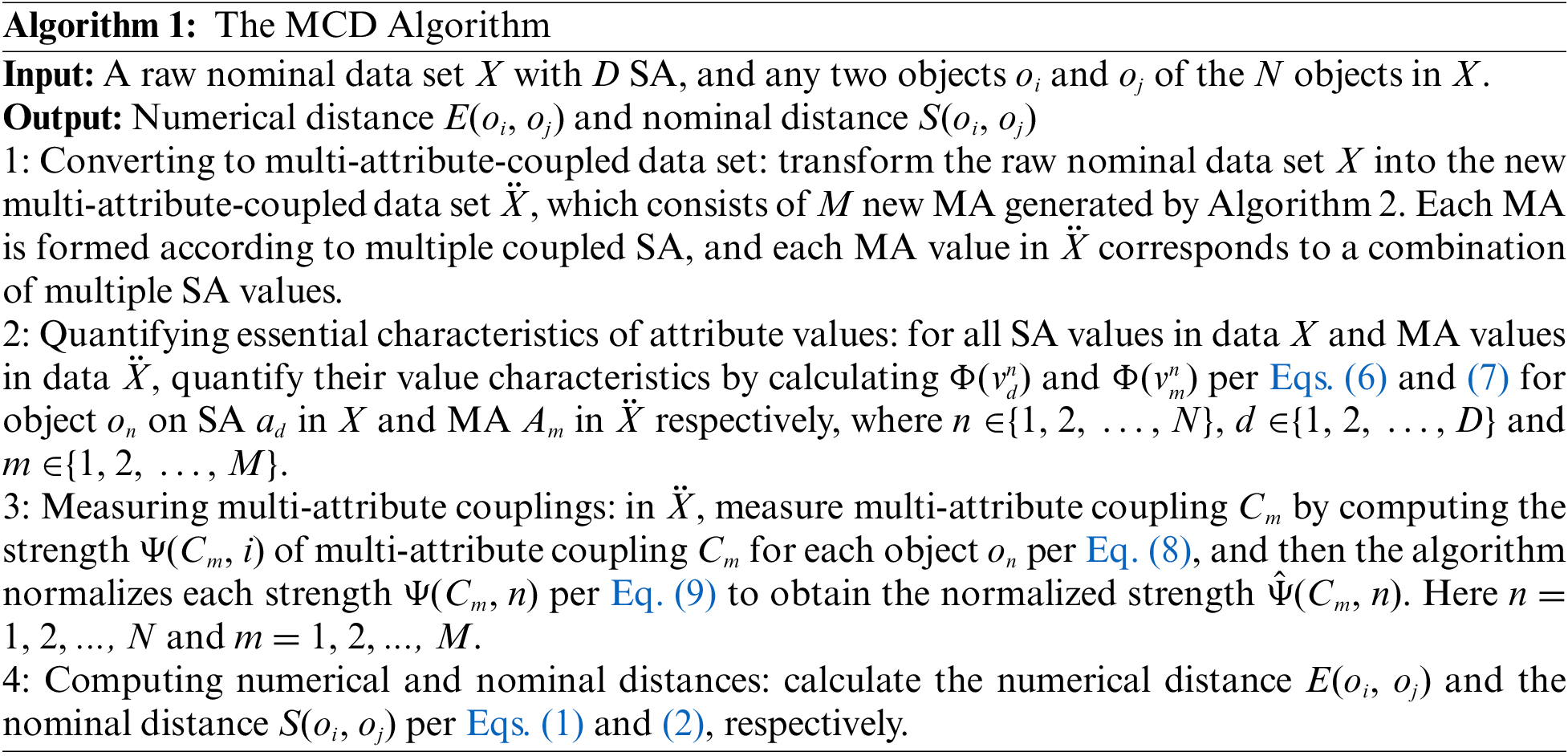
Algorithm 1 summarizes the working process of calculating the multi-attribute couplings-based distances from both nominal and numerical perspectives. It works as follows. First, the raw nominal data set X (such as in Table 2) is converted to a multi-attribute-coupled data set X¨ with two to multiple SA coupled as compound attributes of the new X¨ (as shown in the information Table 3). Second, the algorithm quantifies essential characteristics of both the SA values in the raw data set and the MA values in the new data set regarding self-information and entropy. Further, the strengths of each multi-attribute coupling for each object are calculated and normalized to measure multi-attribute couplings. Lastly, the numerical and nominal distances between any two objects are calculated.

4.2 Converting to Multi-Attribute-Coupled Data set

In Algorithm 1, the first step is to convert the raw data set X to a multi-attribute-coupled data set X¨. X¨ is generated through two procedures: one is to generate M new MA with each of them corresponding to a coupling between SA in the data set X, the other is to assign the MA values to each nominal object.

The first procedure uses Algorithm 2 to produce M new MA, where each new MA represents a coupling between two or multiple SA in the raw data set X. Step 5 is the key of Algorithm 2. In the raw data set X, Step 5 employs a feature selection method (any feature selection method appropriate for nominal attributes) to select t SA. In our work, the feature selection based on the Normalized mutual Information Rank (NIR) is conducted. The normalized mutual information [26] is calculated between aσ (σ∈{1, 2, …, N}) and other attributes in U\{aσ} (i.e., the set of SA except attribute aσ), and then the algorithm chooses t SAs corresponding to the top t highest normalized mutual information. Furthermore, while our work focuses on unlabeled nominal data, Step 5 is also customized for labeled nominal data. For example, a minimal Redundancy-Maximal Relevance (RMR) feature selection method [27,28] can choose features with minimal redundancy and maximal joint relevance to the class labels for classification. In the unlabeled case, the algorithm can also use RMR in Step 5 by substituting class labels with SA aσ to find t SA distinct from aσ and have minimal redundancy and maximal joint relevance to aσ. In practice, an incremental search method can find the near-optimal single-value nominal attributes selected by the RMR. Algorithm 2 generates two kinds of MA w.r.t. entropy. In one case, if a MA has N different values on N objects, MA values follow a discrete uniform distribution, and the entropy of this MA is maximum. In another case, when a MA has one unique value, its entropy is minimum, i.e., 0. These two cases challenge the quantification of the basic characteristics of attribute values for MCD to be grounded on the self-information and attribute entropy mentioned, such as incurring completely identical basic characteristics of all values and zero in the denominator in Eq. (7). To avoid these two cases, in Algorithm 2, Step 12 remove such MA from U¨. In addition, the parameter q controls the number of MA and the number of SA coupled in a derived MA, i.e., any derived MA can be composed of q SA at most. For example, in Table 3, when q = 2, A1 = {a1, a2}, A2 = {a1, a4} and A3 = {a2, a3}; when q = 3, the same A1, A2 and A3 are obtained, but A4={a1,a2,a4}. Steps 7–9 avoid to repeat MA in U¨. For special cases, when D = 2 or D = 1, q = 1 is set and then treat the whole U in X as a new MA in X¨. The second procedure is to assign new MA values to each object. As shown in Definition 2 and Definition 3, a multi-attribute coupling results in a MA derived from multiple original SA. Accordingly, each object receives a set of values corresponding to the individual SA in each newly derived MA. For an object on, one of its newly derived MA Am is composed of two original SA aσ and aη, i.e., Am = {aσ, aη}. The values of aσ and aη on object on are vσn and vηn, then the value of Am is Vθn, i.e., Vθn = {vσn, vηn}. For example, in Table 3, A4 = {a1, a2, a4}, v15 = l4, v25 = c3 and v45 = b1, and thus, V45 = {v15, v25, v45} = {l4, c3, b1}.

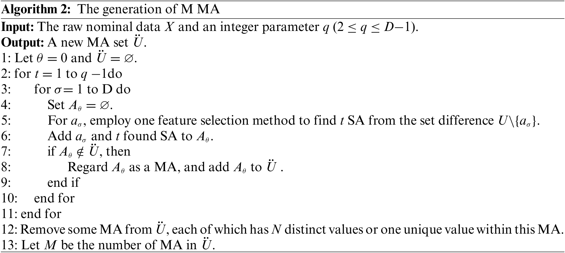
After the two procedures above, the algorithm can obtain a new multi-attribute-coupled data set X¨ (i.e., a new data set) with M MA to describe all nominal objects. Each MA Am and its values were composed of multiple coupled SA and their value combination respectively. Accordingly, in the new data setX¨, each object is described by M multi-attribute couplings Cm.

In X¨, for each object, the number of the captured multi-attribute couplings is dominated by the parameter q in Algorithm 2. Since the more significant q can produce the larger M, the number of the captured multi-attribute couplings related to one object grows with the increase of q. For example, for the raw data set X in Table 2, when q = 2, the newly derived data set X¨ has six objects, each corresponding to 3 two-attribute couplings, i.e., C1, C2 and C3. However, when q = 3, as shown in Tables 3, 4 multi-attribute couplings, i.e., C1, C2, C3 and C4, are allocated to each object in X¨. M generally satisfies 1 ≤ M ≤ (q−1)·D.

Existing distance metrics (e.g., HJM_NDM and CMS_NDM) do not consider the couplings between more than two SA, and these captured attribute couplings only reflect the relationships between two values in one same SA or two different SA. Unlike these distance metrics, our proposed MCD is based on the couplings between two to multiple SA. A multi-attribute coupling captured by MCD can describe the relationships between q~ values in corresponding different q~ SA, and here, 2 ≤ q~ ≤ q. For example, according to X in Table 2, when q = 2, the captured two-attribute couplings form three 2-value attributes A1, A2 and A3 in Table 3, and thus the object o1 in the derived multi-attribute-coupled data set X¨ of Table 3 is only relevant to the combinations of pairwise SA values, that is {l1, c1}, {l1, b4} and {c1, g1}. When q = 3, four captured two- and three-attribute couplings form MA A1, A2, A3 and A4, and thus four MA values {l1, c1}, {l1, b4}, {c1, g1} and {l1, c1, b4} are assigned to object o1 in X¨, corresponding to 2- and 3-value combinations of the constituent SA values respectively.

4.3 Quantifying The Characteristics of Attribute Values

Before measuring the multi-attribute couplings, the algorithm need to capture the basic characteristics of MA and SA values, which can reveal the multi-attribute coupling information hidden in nominal objects. Similar to IDF_NDM, MCD also uses self-information as a quantitative measure of the intrinsic characteristics of each nominal attribute value. Assume h is a value of attribute p in any one nominal data set with N objects. The self-information of value t can be computed by

ϕ(h)=−log(φ(h))(3)

where the default base of the logarithm is two and φ(h) is the occurrence or co-occurrence frequency of h in attribute p. More generally, for the raw data set X and its multi-attribute-coupled representation X¨, the self-information ϕ(vdn) of the SA value vdn of the object on in X is

ϕ(vdn)=−log(φ(vdn))(4)

and the self-information ϕ(Vmn) of the MA value Vmn of the object on in X¨ is

ϕ(vmn)=−log(φ(vmn))(5)

Here, φ(vdn) and φ(Vmn) are the occurrence frequency of SA value vdn and MA value Vmn for all the objects respectively, and φ(Vmn) is also regarded as the co-occurrence frequency of multiple SA values coupled in newly derived MA value Vmn for all the objects.

However, although the value self-information presents the number of intrinsic characteristics of a value, an attribute value can only express objects based on one specific aspect; in contrast, the attribute (with all values) can describe objects from multiple aspects of characteristics. Therefore, this paper combines the entropy ψ(p) of one nominal attribute p with the self-information ϕ(h) of one value h in p as the attribute value’s essential characteristic, i.e., Φ(h). Φ(h) can reveal more information about attribute value h than ϕ(h) because the attribute’s entropy ψ(p) portrays the global characteristic of attribute p.

Definition 4. [A SA value’s essential characteristic] Given a SA ad and its value vdn on any object on, Φ(vdn) is the essential characteristic of this value, which can be defined as:

Φ(vdn)=ϕ(vdn)ψ(ad)(6)

where ϕ(vdn) is the self-information of value vdn, ψ(ad) is the entropy of SA ad, n∈{1, 2, …, N} and d∈{1, 2, …, D}.

Definition 5. [A MA value’s essential characteristic] Given a MA Am and its value Vmn on any object on, Φ(Vmn) is the essential characteristic of this value, which can be defined as:

Φ(vmn)=ϕ(Vmn)ψ(Am)(7)

where ϕ(Vmn) is the self-information of value Vmn, ψ(Am) is the entropy of MA Am, n∈{1, 2, …, N} and m∈{1, 2, …, M}.

For example, for SA value v21 (v21 = c1) in Table 2, ϕ(v21) = 2.5850, ψ(a2) = 1.4591 and Φ(v21) = 1.7716 are computed. While for the newly derived MA value V45 (V45 = {l4, c3, b1}) in Table 3, ϕ(V45) = 1.5850, ψ(A4) = 2.2516 and Φ(V45) = 0.7039. Furthermore, in Definition 5, for X¨, ψ(Am)≠0 because Step 12 of Algorithm 2 removes multi-value attribute Am, the entropy of which is equal to 0. However, in Definition 4, for the raw data set X, ψ(ad) may be 0. If this is the case, let Φ(vdn) = 1/N.

4.4 Measuring Multi-Attribute Couplings

The multi-attribute-coupled data representation determines what multi-attribute couplings are embedded for objects in the raw data set. Thus, the strength of a multi-attribute coupling is determined by the strength of this coupling for each object. Moreover, a multi-attribute coupling determines an interaction of multiple SA, reflects the relationships between multiple coupled SA values in respective different SA, and further forms a new MA and the values of this MA. Consequently, according to the essential characteristics of SA and MA values, this paper defines the strength of a multi-attribute coupling for one object as follows.

Definition 6. [The strength of a multi-attribute coupling for one object] Given a raw nominal data set X, a multi-attribute-coupled data set X¨ that is a constructed data set and converted from X, and a value Vmn of MA Am on object on in X¨, the strength of multi-attribute coupling Cm for object on is Ψ(Cm, n), which is defined as:

Ψ(Cm,n)=Φ(vdn)∏∀vmn∈VmnΦ(vdn)(8)

where n∈{1, 2, …, N} and m∈{1, 2, …, M}, vdnis the value of SA ad on object on in the raw X (d=1, 2, …, D) and Vmn is the combination of multiple SA values.

Moreover, the obtained strengths should be normalized to cope with different scales of distance metrics. A normalized strength of a multi-attribute coupling Cm for one object on is given as follows:

Ψ^(Cm,n)=Ψ(Cm,n)ω(Cm)(9)

where Ψ(Cm, n) can be calculated per Eq. (8) and ω(Cm) is the sum of all the different strengths of multi-attribute couplings Cm for all objects.

For example, A4 = {a1,a2,a4} and V45 = {l4, c3, b1} in Table 3. To calculate the normalized strength of three-attribute coupling C4 for object o5, the algorithm can respectively obtain SA and MA value’s essential characteristics Φ(v15) = Φ(l4) = 0.8262, Φ(v25) = Φ(c3) = 0.6853, Φ(v45) = Φ(b1) = 0.5579 and Φ(V45) = 0.7039 (Φ(V45) = Φ({l4, c3, b1})) per Eq. (6) and Eq. (7), and further, Ψ(C4, 5) = 0.2224 is obtained per Eq. (8). Since there are five different strengths of multi-attribute coupling C4 for all six objects, i.e., Ψ(C4,1), Ψ(C4,2), Ψ(C4,3), Ψ(C4,5) (Ψ(C4,4) = Ψ(C4,5)) and Ψ(C4,6), finally, the sum ω(C4) = Ψ(C4,1)+Ψ(C4,2) + Ψ(C4,3) + Ψ(C4,5) + Ψ(C4,6) = 7.5355 and the normalized strength Ψ^(C4,5) = 0.0295 are calculated per Eq. (9).

5  Experiments

In this section, this paper evaluates the proposed MCD distance metrics on 15 numerical and nominal data sets, compares MCD with directly relevant baselines, and analyzes the performance of MCD.

5.1 Data Sets

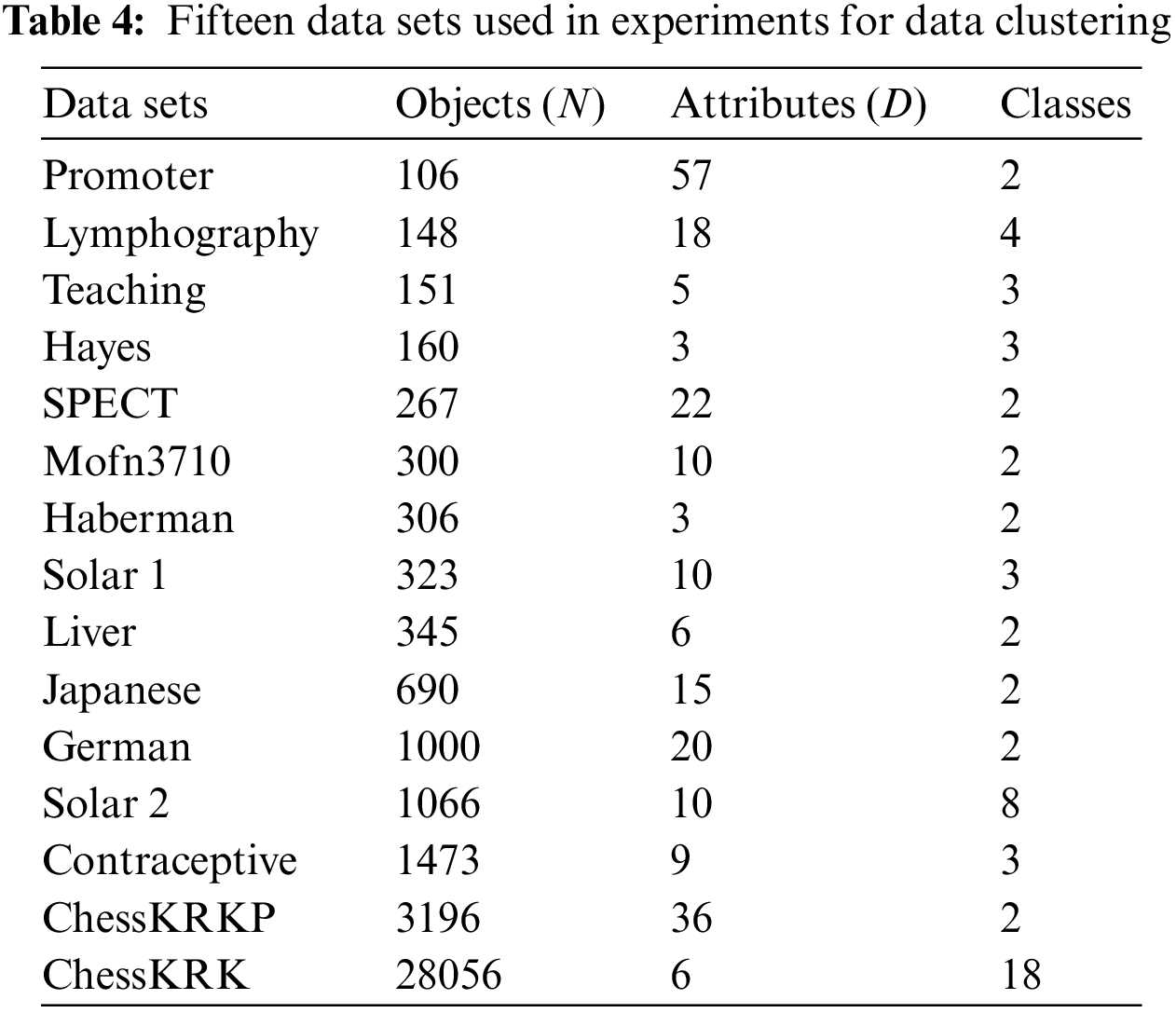
15 UCI data sets [29] were used in our experiments: Promoter Gene Sequences (Promoter for short), Lymphography Data (Lymphography), Teaching Assistant Evaluation (Teaching), Hayes-Roth (Hayes), SPECT Heart Data Set (SPECT), Mofn-3-7-10(Mofn3710), Haberman’s Survival Data (Haberman), Solar Flare Data1 (Solar 1), Liver Disorders (Liver), Japanese Credit Screening (Japanese), German Credit Data (German), Solar Flare Data2 (Solar 2), Contraceptive Method Choice (Contraceptive), Chess (King-Rook vs. King-Pawn) (ChessKRKP), and Chess (King-Rook vs. King) (ChessKRK). For data sets with numerical attributes, this paper discretizes and converts their numerical attributes to nominal ones. Table 4 summarizes the main data factors.

5.2 Baseline Distances for Clustering

MCD is evaluated w.r.t. the following aspects: (1) The comparison with seven state-of-the-art distance measures: DV_EDM, HAM_NDM, IDF_EDM, CDE_EDM, RMF_NDM, HJM_NDM and CMS_NDM, which are chosen as distance baselines. (2) The flexibility of MCD as both numerical and nominal distances: as shown in Algorithm1, MCD can serve as both Euclidean (EDM) and nominal (NDM) distance metrics for nominal data clustering per Eqs. (1) and (2), resulting in two distance metrics MC_EDM and MC_NDM. (3) The influence of feature selection on multi-attribute couplings: MCD requires feature selection to filter less relevant multi-attribute couplings, and this paper applies two filtering methods, NIR and RMR, in Step 5 of Algorithm 2, further resulting in the following four MCD distance metrics: MC_EDM-NIR, MC_EDM-RMR, MC_NDM-NIR, and MC_NDM-RMR. In addition, this paper evaluates the MCD applicability to clustering. As our purpose is not to design a novel robust clustering algorithm, but to test the performance of the proposed distance metrics to enable better clustering for both numerical and nominal data, this research incorporates MCD distances into two kinds of clustering methods, i.e., unique nominal clustering methods and numerical clustering methods. The number of the former is minimal, and thus, the most popular K-modes [8] are chosen and incorporated with every NDM-type distance to cluster nominal data set. For the latter, the most classic method, i.e., K-means [30,31], is chosen and incorporated with every EDM-type distance to cluster the transformed numerical data set.

The distance measures are suitable for the nominal data set, incorporated into K-modes, and compared in the following experiments: HAM_NDM, RMF_NDM, HJM_NDM, CMS_NDM, the proposed MC_NDM-NIR, and MC_NDM-RMR. In the contrast, the distance measures are Euclidean compatible, incorporated into K-means, and compared in the experiments as follows: DV_EDM, IDF_EDM, CDE_EDM, the proposed MC_EDM-NIR, and MC_EDM-RMR

5.3 Evaluation Methods and Parameter Settings

First, for a fair comparison between all distance measures, the cluster number is set as the number of classes in each data set. Two commonly used evaluation criteria for clustering are taken here: F-score and the normalized mutual information (NMI) [26]. The reported results of the F-score and NMI are averaged on 100 independent runs on each data set. The larger values of the F-score and NMI indicate better clustering performance.

Second, some baseline metrics require parameters such as HJM_NDM, CMS_NDM, and CDE_EDM. CDE_EDM is insensitive to parameters [32], and this paper takes the best parameters recommended by their authors of HJM_NDM and CMS_NDM in [6] and [7] respectively. MCD involves one parameter q which is an integer number and can be chosen by satisfying the condition2 ≤ q ≤ D−1, where D is the number of the original SA in each nominal data set.

5.4 Influence of The Number of Multi-Attribute Couplings

In converting a raw data set to a multi-attribute-coupled data set for calculating MCD, the number of MA is restricted by the parameter q in terms of Algorithm 2. Since a captured multi-attribute coupling can produce a MA, the parameter q is also used to regulate the number of multi-attribute couplings, and generally, the number of multi-attribute couplings grows with the increase of q. The 15 experimental data sets have different numbers of SA, i.e., D is different for each data set. To better present the influence of q (2≤q≤D−1),letq=⌈β(D−1)⌉(β={0,0.2,0.4,0.6,0.8}) in MCD. If ⌈β(D−1)⌉<2,q=2 is set here. In this way, obviously, the bigger β can lead to the more extensive q, which can involve more multi-attribute couplings. Multi-attribute couplings serve as the kernel stone of our proposed MCD and reflect the relationships between the values in respective multiple SA. More multi-attribute couplings can bring about more relations in MCD. Below, experiments show the influence of the number of multi-attribute couplings on the clustering performance when incorporating MCD into a clustering algorithm.

Fig. 1 depicts that more multi-attribute couplings can enhance the clustering performance of MCD. The F-score results obtained by MC_NDM-NIR and MC_NDM-RMR in K-modes clustering w.r.t. different values of β are respectively given on 15 data sets. Fig. 1 shows that the F-score results of both MC_NDM-NIR and MC_NDM-RMR on 13 of all 15 data sets keep growing when the value of β increases. Fig. 1 also presents that the results of the F-score of both MC_EDM-NIR and MC_EDM-RMR in K-means clustering on 11 of all 15 data sets grow with the increase of β. The F-score on Hayes and Haberman remains unchanged because these data sets only have three original SA, i.e.,D = 3. Hence q is permanently fixed to 2.

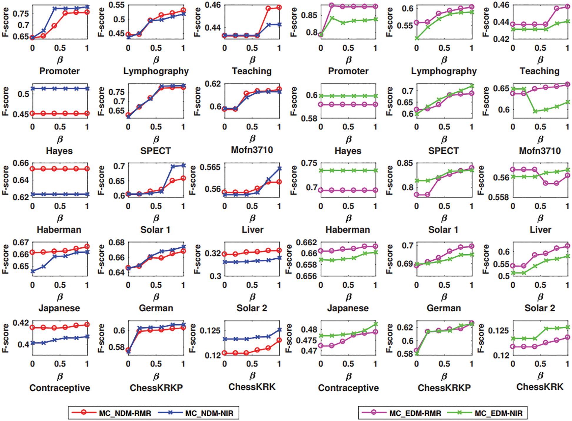
Figure 1: F-score based on distances MC_NDM-RMR and MC_NDM-NIR with different parameters in K-modes clustering, and F-score based on distances MC_EDM-RMR and MC_EDM-NIR with different parameters in K-means clustering

5.5 Comparison of Different Distances-Driven Clustering Performance

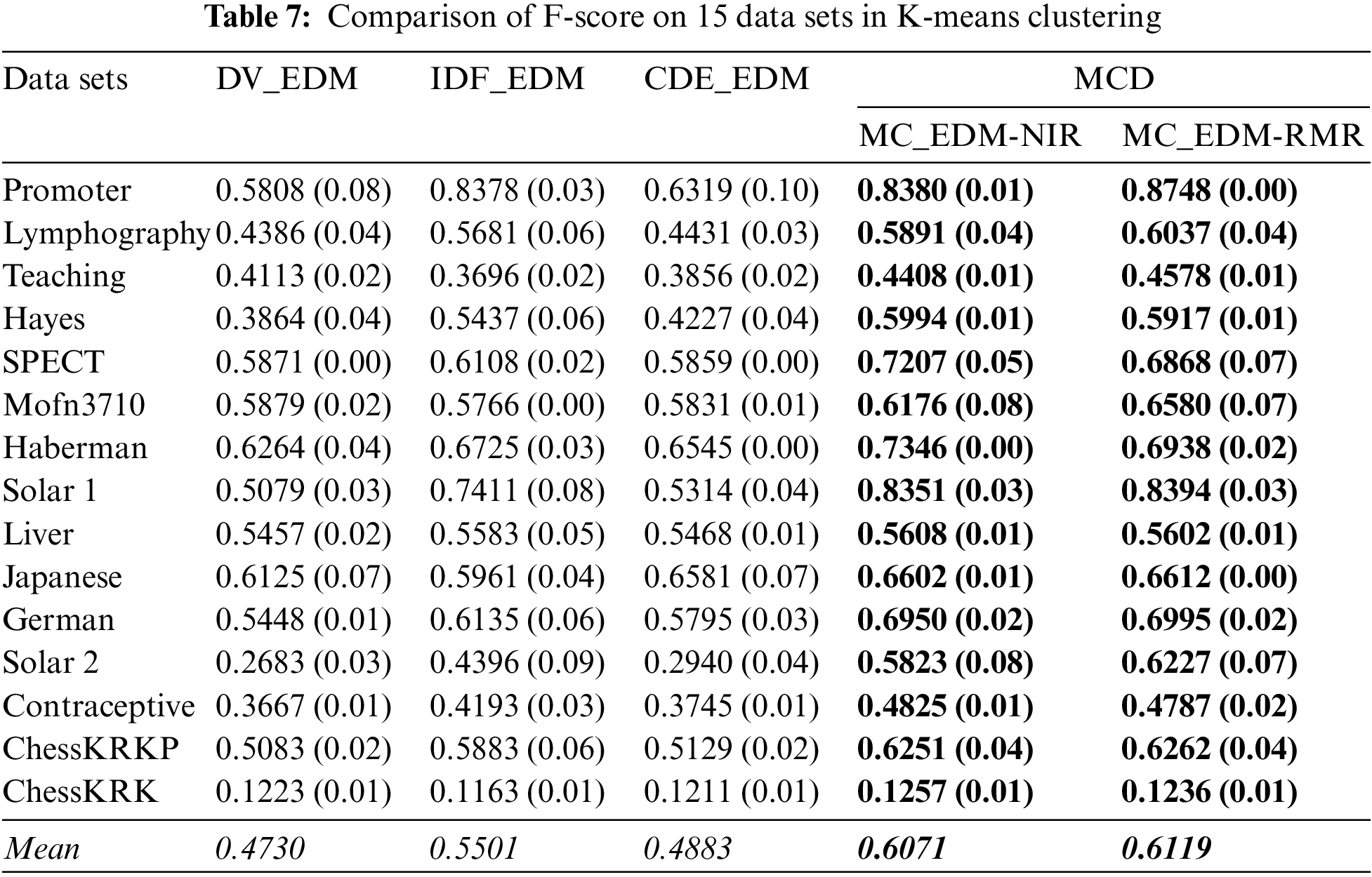
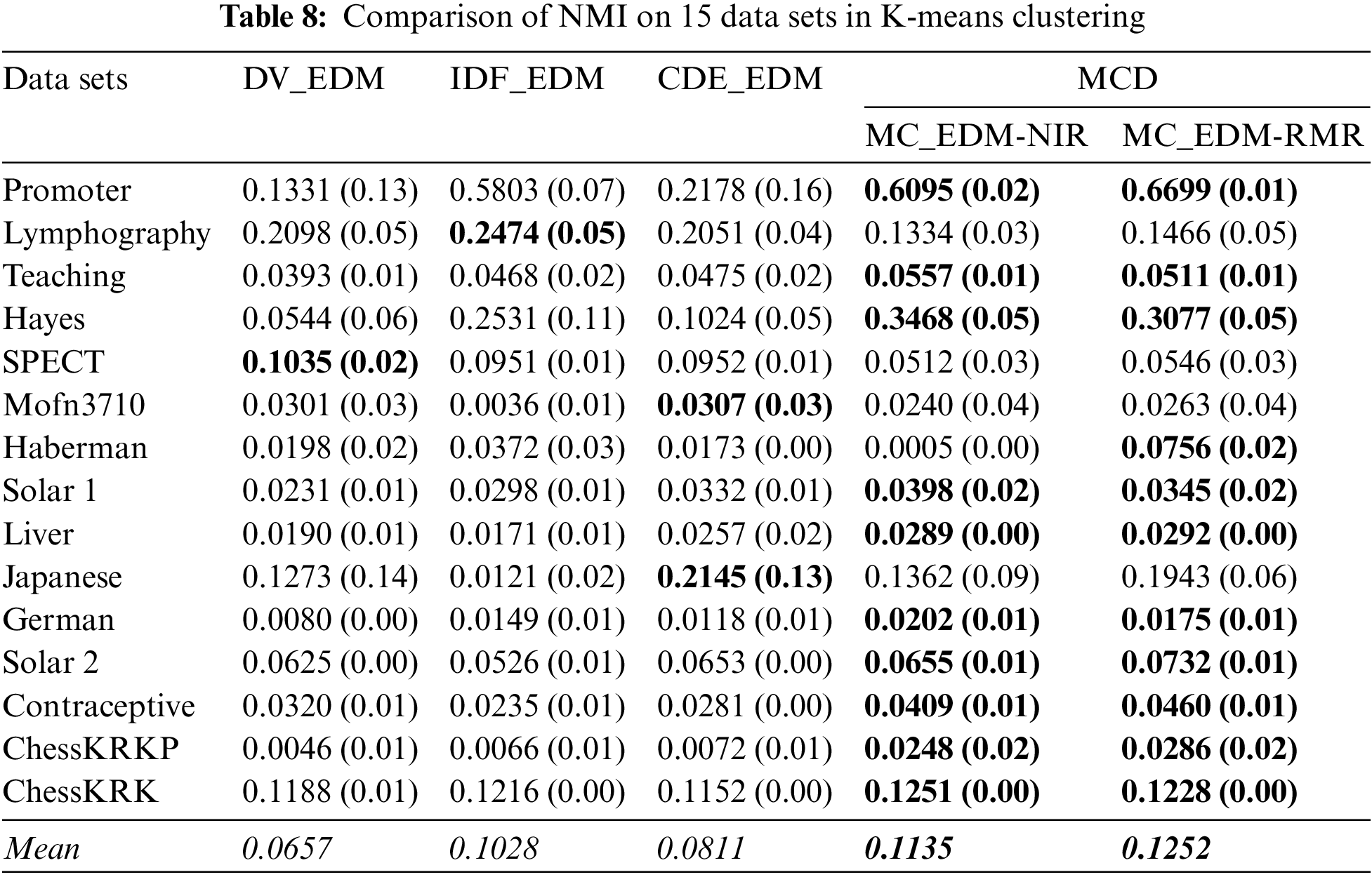
Here, this paper compares the clustering performance in terms of the baseline distances and the multi-attribute coupling-driven MCD for clustering. This paper sets q = D−1 and then applies this q to MCD for experiments. The averaged F-score and NMI values, as well as their standard deviations (values in parentheses) on 15 data sets, are reported in Tables 5–8, respectively. The better clustering performance is marked in boldface, and the overall performance is noted in italic in the bottom row w.r.t. the mean value.

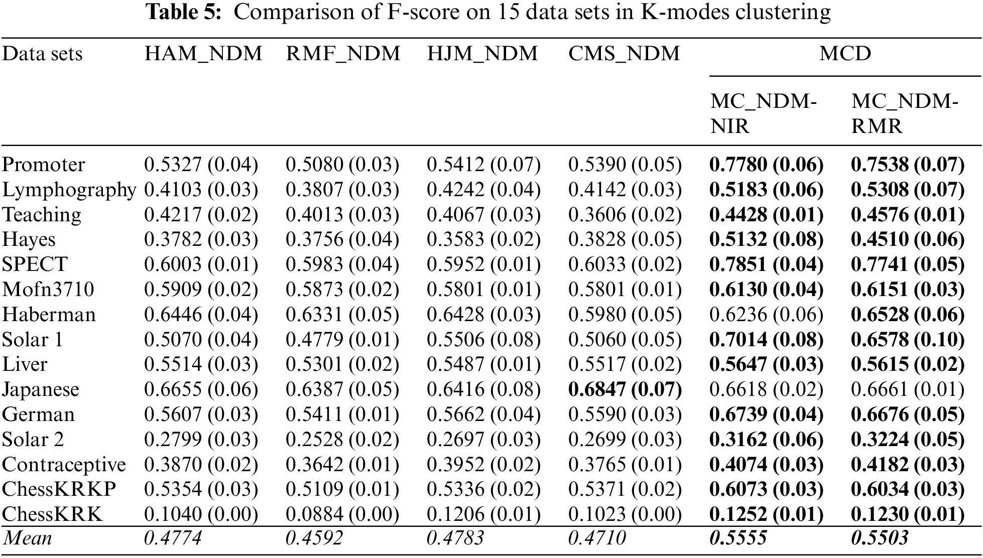
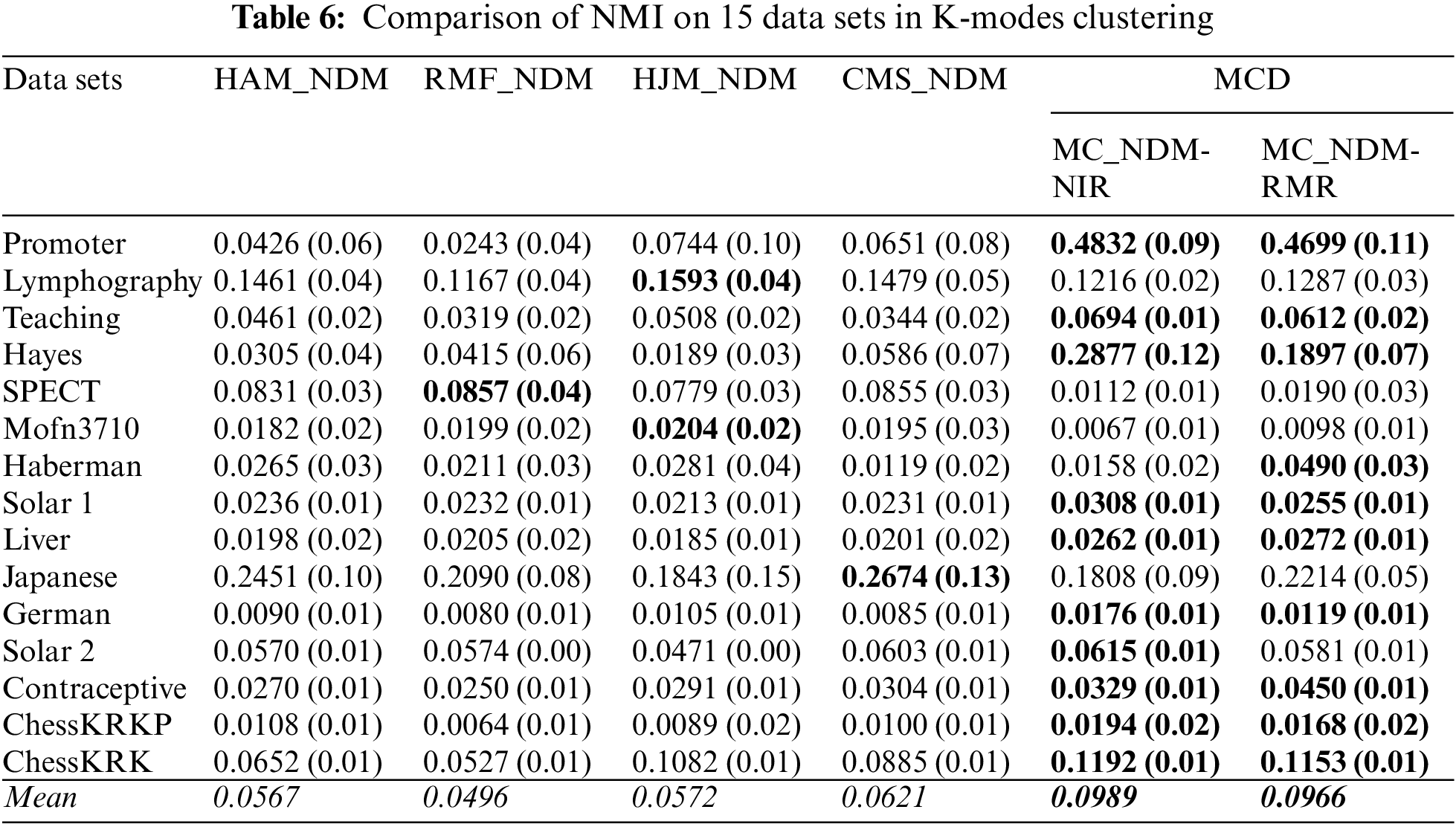
First, Tables 5 and 6 show that two baselines, HJM_NDM and CMS_NDM, present better mean F-score and NMI in all four baselines based on NDM, respectively. In particular, CMS_NDM achieves the best F-score and NMI in comparison with MC_NDM-NIR, MC_NDM-RMR, and other baselines on the data set Japanese. However, MC_NDM-NIR and MC_NDM-RMR not only outperform the four baselines on the overall clustering performance but also work well on more data sets. For example, the F-score of MC_NDM-NIR and MC_NDM-RMR is more significant than that of the baselines on 13 and 14 data sets, respectively. In contrast, MC_NDM-NIR and MC_NDM-RMR underperform the baselines w.r.t. NMI on only five data sets.

Second, as shown in Tables 7 and 8 although DV_EDM obtains the best NMI on the data set SPECT, both their mean F-score and mean NMI is inferior to two homogeneous methods, IDF_EDM and CDE_EDM. The mean values of MC_EDM-NIR and MC_EDM-RMR indicate that they are more competent for nominal data clustering than the baselines. The F-score of both MC_EDM-NIR and MC_EDM-RMR is much better than that of baselines on all data sets. Furthermore, except for five data sets, the NMI of MC_EDM-NIR consistently outperforms that of the baselines on the other 10 data sets, and except for four data sets, the NMI of MC_EDM-RMR always beats that of the baselines on 11 remaining data sets.

Last, this research finds that distinct feature selection methods taken in Algorithms 2 do not reflect the significant differences in final clustering performance. When MC_NDM-NIR is compared with MC_NDM-RMR, Tables 5 and 6 show that MC_NDM-NIR achieves the unsatisfactory F-score and NMI on seven of all 15 data sets. When MC_EDM-NIR is compared with MC_EDM-RMR, Table 7 shows that MC_EDM-NIR achieves a very good F-score on 6 of all data sets, and in Table 8, MC_EDM-NIR performs worse than MC_EDM-RMR on 10 of all data sets.

6  Conclusions and Future Work

Learning unlabeled nominal data is much more challenging than the numerical one due to the more diversified characteristics embedded in nominal data. Recent years have seen increasing efforts to design more effective distance measures for nominal data by capturing specific complexities, e.g., co-occurring frequency and attribute couplings. Existing work typically takes a pairwise approach to model value relations and two-attribute couplings in nominal data and then measures the dissimilarity between objects. This paper explores the couplings between two to multiple attributes in nominal data and designs two multi-attribute couplings-based distance (MCD) metrics that (1) capture the couplings between multiple attributes by converting a raw nominal data set to a new multi-attribute-coupled data set, i.e., a multi-attribute-coupled representation; (2) quantify attribute value’s essential characteristics by using the value self-information and attribute entropy; (3) measure multi-attribute couplings and obtain their strengths for efficient computation; and (4) enable the applications of both numerical and specific nominal clustering methods on nominal data. Our experiments on 15 data sets compared to seven state-of-the-art distance measures and the MCD variants by embedding different feature selection methods show that MCD delivers superior clustering performance for both numerical and nominal clustering tasks. In the future, our research will work on optimizing the selection of high-dimensional attribute couplings and designing new data structures and methods to calculate the multi-attribute-coupled value similarity and object similarity on high-dimensional and large-scale data. Moreover, our works will be considered to be applied to other fields such as real physical systems and quantum information processing.

Funding Statement: This work is funded by the MOE (Ministry of Education in China) Project of Humanities and Social Sciences (Project Number: 18YJC870006) from China.

Conflicts of Interest:: The authors declare that they have no conflicts of interest to report regarding the present study.

References

1. A. Agresti, “An introduction to categorical data analysis,” in Wiley Series in Probability and Statistics, Hoboken, New Jersey, US: John Wiley & Sons, Inc, 2007. [Google Scholar]

2. L. Cao, “Couping learning of complex interactions,” Information Processing & Management, vol. 51,no. 2, pp. 167–186, 2015. [Google Scholar]

3. L. Cao, “Non-iidness learning in behavioral and social data,” The Computer Journal, vol. 57, no. 9, pp. 1358–1370, 2014. [Google Scholar]

4. H. Bock and E. Diday, “Analysis of symbolic data: Exploratory methods for extracting statistical information from complex data,” in Studies in Classification, Data Analysis, and Knowledge Organization, New York, US: Springer, 2000. [Google Scholar]

5. F. Cao, J. Liang, D. Li, L. Bai and C. Dang, “A dissimilarity measure for the k-modes clustering algorithm,” Knowledge-Based Systems, vol. 26, no. 5, pp. 120–127, 2012. [Google Scholar]

6. H. Jia, Y. M. Cheung and J. Liu, “A new distance metric for unsupervised learning of categorical data,” IEEE Transactions on Neural Networks and Learning Systems, vol. 27, no. 5, pp. 1065–1079, 2016. [Google Scholar] [PubMed]

7. S. Jian, L. Cao, K. Lu and H. Gao, “Unsupervised coupled metric similarity for non-iid categorical data,” IEEE Transactions on Knowledge and Data Engineering, vol. 30, no. 9, pp. 1810–1823, 2018. [Google Scholar]

8. Z. Huang, “Extensions to the k-means algorithm for clustering large data sets with categorical values,” Data Mining and Knowledge Discovery, vol. 2, no. 3, pp. 283–304, 1998. [Google Scholar]

9. E. Zdravevski, P. Lameski, A. Kulakov and S. Kalajdziski, “Transformation of nominal features into numeric in supervised multiclass problems based on the weight of evidence parameter,” in Proc. FedCSIS, Lodz, Poland, pp. 169–179, 2015. [Google Scholar]

10. M. Berry, Survey of Text Mining: Clustering, Classification, and Retrieval. New York: in Springer, 2003. [Google Scholar]

11. S. Jian, G. Pang, L. Cao, K. Lu and H. Gao, “Cure: Flexible categorical data representation by hierarchical coupling learning,” IEEE Transactions on Knowledge and Data Engineering, vol. 31, no. 5, pp. 853–866, 2019. [Google Scholar]

12. C. Liu, L. Cao and P. S. Yu, “Coupled fuzzy k-nearest neighbors classification of imbalanced non-iid categorical data,” in Proc. Int. Joint Conf. on Neural Networks (IJCNN), Beijing, China, pp. 1122–1129, 2014. [Google Scholar]

13. C. Wang, Z. She and L. Cao, “Coupled attribute analysis on numerical data,” in Proc. the 23rd Int. Joint Conf. on Artificial Intelligence (IJCAI), Beijing, China, pp. 1736–1742, 2013. [Google Scholar]

14. S. Jian, L. Hu, L. Cao and K. Lu, “Metric-based auto-instructor for learning mixed data representation,” in Proc. the Thirty-Second AAAI Conf. on Artificial Intelligence (AAAI), New Orleans, Louisiana, USA, pp. 3318–3325, 2018. [Google Scholar]

15. G. Pang, L. Cao, L. Chen, D. Lian and H. Liu, “Sparse modeling-based sequential ensemble learning for effective outlier detection in high-dimensional numeric data,” in Proc. the Thirty-Second AAAI Conf. on Artificial Intelligence, (AAAI), New Orleans, Louisiana, USA, pp. 3892–3899, 2018. [Google Scholar]

16. Q. Chen, L. Hu, J. Xu, W. Liu and L. Cao, “Document similarity analysis via involving both explicit and implicit semantic couplings,” in Proc. IEEE Int. Conf. on Data Science and Advanced Analytics (DSAA), Paris, France, pp. 1–10, 2015. [Google Scholar]

17. J. Xu and L. Cao, “Vine copula-based asymmetry and tail dependence modeling,” in Proc. the Pacific-Asia Conf. Knowledge Discovery and Data Mining, Melbourne, Australia, pp. 285–297, 2018. [Google Scholar]

18. Y. Song, L. Cao, X. Wu, G. Wei, W. Ye et al., “Coupled behavior analysis for capturing coupling relationships in group-based market manipulations,” in Proc. the 18th ACM SIGKDD Int. Conf. on Knowledge Discovery and Data Mining, New York, USA, pp. 976–984, 2012. [Google Scholar]

19. J. G. Proakis and M. Salehi, “Communication Systems Engineering,” in Upper Saddle River, 2nd edition, NJ, USA: Prentice-Hall, 2001. [Google Scholar]

20. T. R. L. dos Santos and L. Zarate, “Categorical data clustering: Hat similarity measure to recommend?,” Expert Systems with Applications, vol. 42, no. 3, pp. 1247–1260, 2015. [Google Scholar]

21. A. Ahmad and L. Dey, “A method to compute distance between wo categorical values of same attribute in unsupervised learning or categorical data set,” Pattern Recognition Letters, vol. 28, pp. 10–118, 2007. [Google Scholar]

22. S. Q. Le and T. B. Ho, “An association-based dissimilarity measure or categorical data,” Pattern Recognition Letters, vol. 26, no. 16, pp. 549–557, 2005. [Google Scholar]

23. D. Ienco, R. Pensa and R. Meo, “From context to distance: Learning dissimilarity for categorical data clustering,” ACM Transactions on Knowledge Discovery from Data, vol. 6, no. 1, pp. 1–25, 2012. [Google Scholar]

24. C. Wang, L. Cao, M. Wang, J. Li, W. Wei et al., “Coupled nominal similarity in unsupervised learning,” in Proc. the 20th ACM Conf. on Information and Knowledge Management (CIKM), Glasgow, UK, pp. 973–978, 2011. [Google Scholar]

25. C. Wang, X. Dong, F. Zhou, L. Cao and C. -H. Chi, “Coupled attribute similarity learning on categorical data,” IEEE Transactions on Neural Networks and Learning Systems, vol. 26, no. 4, pp. 781–797, 2015. [Google Scholar] [PubMed]

26. C. D. Manning, P. Raghavan and H. Schütze, Introduction to information retrieval. New York: Cambridge University Press, 2008. [Google Scholar]

27. C. Ding and H. Peng, “Minimum redundancy feature selection from microarray gene expression data,” in Proc. the IEEE Computer Society Conf. on Bioinformatics, Stanford, USA, pp. 523–528, 2003. [Google Scholar]

28. H. Peng, F. Long and C. Ding, “Feature selection based on mutual information criteria of max-dependency, max-relevance, and min-redundancy,” IEEE Transactions on Pattern Analysis and Machine Intelligence, vol. 27, no. 8, pp. 1226–1238, 2005. [Google Scholar] [PubMed]

29. UCI Machine Learning Repository. 2007. [Online]. Available: https://archive.ics.uci.edu/ml/index.php [Google Scholar]

30. M. Filippone, F. Camastra, F. Masulli and S. Rovetta, “A survey of kernel and spectral methods for clustering,” Pattern Recognition, vol. 41, no. 1, pp. 176–190, 2008. [Google Scholar]

31. R. Xu and D. Wunsch, “Survey of clustering algorithms,” IEEE Transactions on Neural Networks and Learning Systems, vol. 16, no. 3, pp. 645–678, 2005. [Google Scholar]

32. S. Jian, L. Cao and G. Pang, “Embedding-based representation of categorical data by hierarchical value coupling learning,” in Proc. the Twenty-Sixth Int. Joint Conf. on Artificial Intelligence (IJCAI), Melbourne, Australia, pp. 1937–1943, 2017. [Google Scholar]