ML and CFD Simulation of Flow Structure around Tandem Bridge Piers in Pressurized Flow

1  Introduction

Due to increased human pressure on various catchments, severe riverine and coastal floods have become more frequent and powerful. Both urbanization and changes in farming practices are part of this demand. Storm surge, hurricane activity, sea level rise, and other natural processes are all associated with an overall increase in the risk of catastrophic occurrences [1–4]. As a result, many outdated infrastructures, including bridges, were constructed years ago. This led to designs that might not have considered the significant increase in severe incidents [1]. Increases in approach flow depth can result in the bridge deck becoming fully or partially inundated. Flood-inundated bridges are vulnerable to pressured flow conditions, which can exacerbate the scour scenario [5]. In these circumstances, the deck reduces the width of the flow conveyance sections, accelerating and modifying the flow and turbulence structure where the bridge pier resides. This causes more scouring and raises the likelihood of unexpected failures [6].

A thorough study of the flow dynamics around such structures is required to fully comprehend how hydraulic structures affect flow behaviour and sediment transport [7,8]. Flow dynamics and turbulence characteristics around bridge piers and their effect on the characteristics of scour hole is also studied extensively to provide this comprehension [9–11]. Turbulent flow dynamics are often quantified in terms of turbulence intensity, Reynolds stress, and total kinetic energy, with numerous coherent structures forming when a free-surface flow collides with a vertical structure. In the presence of piers, the following elements of vortex shedding were identified: (a) an upward-directed and rotating surface roller; (b) a downward-directed flow that forms in front of the pier, directed toward the pier base; (c) a horseshoe vortex at the bridge pier base, which has a significant effect on the scour morphology; and (d) wake vortices downstream of the bridge pier [1]. Even though the scour hole and the design methods for pressure flow conditions are studied extensively (i.e., see [12–14] ), the velocity field in the pressure-flow state is studied in only a handful of research. Reference [15] utilized experimental facilities to explore the vertical velocity profile along the centerline in vertical contraction-induced pressure-flow scour. The highest velocity was observed towards the midpoint of the vertical profile downstream of the bridge.

Additionally, he reported that the scouring happened, although the average velocity at any segment did not reach the critical velocity. Lin et al. [16] studied the flow structure under a partially submerged inundated bridge deck. They classified the flow under the bridge into four categories, including (type I) with the downstream flow elevation slightly lower than the upstream, the flow is tangent to the deck and the shear layer created at the bottom of the upstream girder varies continually and contacts the soffit of all girders; (type 2) flow level at downstream is significantly lower than the upstream, and the shear layer generated by the upstream girder collides the third cavity between the girders; (type 3) when the shear layer is separated from the upstream girder forming a jet flow which impacts all the girders; and (type 4) which is similar to an orifice flow under the bridge deck with flow fully detached from the deck bottom. Yoon et al. [17] studied the velocity field through simultaneous bridge lateral and vertical contractions in pressurized flow conditions using a 1:60 scaled model of the Towa Liga river bridge at Macon, Georgia, USA. Their findings indicate that, in addition to the local turbulence structure wrapping around the base of the abutment, the highest scour occurs near the abutment owing to the increased cross-sectional velocity caused by the local flow acceleration. They have also mentioned the variation between the velocity field in free surface flow and the submerged zone. It is also confirmed that the zone of the maximum velocity tends to shift toward the mid-depth and closer to the channel bed. Considering the fact that flow structure around tandem piers or groups of piers is significantly different from single piers and scour depth around pile groups could exceed twice that of single piers [18]. Further research has focused on the study of peer groups, i.e., [18,19]. Wang and Liang, 2020 introduced a new approach for calculating scour in layered soils based on the equilibrium concept and considering the geo-mechanical properties of the soils with different resistance to erosion. Through numerical simulations, Kim, 2014 discovered that the maximum depth of scour around tandem double-pier structures increases first with the distance between them and then decreases gradually as the distance between them grows until it reaches an equilibrium value.

In summary, many researchers have been studying the flow structure and scour process around single and tandem piers in free-flow conditions, so there is an extravagance of information in this section. Besides, there are valuable studies considering the scour process or flow field in contraction flow conditions, yet to our knowledge, tandem piers in vertical contraction flow conditions are not studied thoroughly. Hence, the current study aims to determine the effect of the deck length to pier width ratio, pier numbers, and pier spacing on the flow structure and bed shear stress in constrained flow circumstances. Thus, using a commercial CFD software, numerical simulations are carried out, and the flow velocity and turbulence elements are compared in various deck length and pier spacing conditions. Finally, five different machine learning algorithms, including the Decision trees [20], Random Forest [21,22], Adaboost regression [23], stacked regression model [24], and Multi-Layer Perceptron (MLP) [25], are implemented and fine-tuned using Bayesian optimisation [26]. The accuracy of the models are then compared concerning estimating the velocity components and the turbulent kinetic energy of the flow at various channel depths.

2  Numerical Modeling

The FLOW-3D numerical model was used to solve the Navier–Stokes equation and obtain fully three-dimensional flow patterns at the channel.

2.1 Governing Equations

The governing equations include momentum and continuity. The continuity equation, regardless of the density of the fluid in the form of Cartesian coordinates x, y, and z, could be described as follows Eq. (1):

VFρc2∂ρ∂t+∂∂x(uAx)+R∂∂y(vAy)+∂∂z(wAz)+ξuAxx=Rsorρ(1)

where u, v, and w denote velocity vectors in the x, y, and z directions; Ax, Ay, and Az mean the surface flow fractions in the x, y, and z, respectively; VF flow volume fraction; the fluid density (ρ); t denotes time, and Rsor represents the mass source. Eq. (2) describes the momentum equation in three dimensions Eq. (2):

∂u∂t+1VF(uAx∂u∂x+vAy∂u∂y+wAz∂u∂z)−ξAyv2xVF=−1ρ∂ρ∂x+Gx+fx−bx−RSORρVF(u−uw−δus)∂vσt+1VF(uAx∂v∂x+vAy∂v∂y+wAz∂v∂z)−ξAyuvxVF=−1ρ(R∂ρ∂y)+Gy+fy−by−RSORρVF(v−vw−δvs)∂w∂t+1VF(uAx∂w∂x+vAy∂w∂y+wAz∂w∂z)=−1ρ∂ρ∂z+Gz+fz−bz−RSORρVF(w−ww−δws)(2)

where Gx , Gy, and Gz denote the gravity-induced accelerations in the x, y, and z axes, respectively; fx, fy, and fz are the accelerations due to viscosity in the x, y, and z directions, respectively. Besides, bx,by, and bz are flow losses in porous media or across porous baffle plates, and the final terms account for the injection of mass at a source represented by a geometry component.

2.2 Turbulence Modeling

The large-eddy simulation (LES) model was applied to simulate the complex turbulent flow field in the region. The Flow-3D application uses the well-known Smagorinsky model for subgrid-scale stresses. The mesh size is considered as the vortex size filter. The characteristics of turbulence that are too subtle to be calculated explicitly are represented in the LES model by an eddy viscosity that is proportional to a length scale multiplied by a measure of velocity variations on that length scale. Flow-3D calculates this length scale by taking the geometric mean of the size of the grid cells as follows Eq. (3):

L=(δxδyδz)13(3)

And then adjusts the amplitude of velocity changes by L times the mean shear stress. These values are added together to get the LES kinematic eddy viscosity Eq. (4):

υT=(cL)2.2eij2eij(4)

where (c) is a constant typically between 0.1 to 0.2, and (eij) indicates the strain rate of tensor components.

2.3 Boundary Conditions and Gridding

The experimental study of Carnacina et al. [1] was adopted as the base for validation and further studies. Experimental facilities include a laboratory flume of 7.6 m length and 0.61 m width. A column with a 0.03 m diameter is also used as the bridge pier. To model the pressurized flow conditions, a plate is placed over the flow to mimic the bridge deck, and the flow height upstream of the bridge deck is set equal to 0.17 cm. In this study, a structured non-uniform mesh block was utilized to discretize the flow field in the channel. The grid domain is denser in the piers and contracted zone area to increase the accuracy of calculations. Boundary conditions comprise inflow discharge for the channel entry, constant level outflow (constant pressure) for the channel outlet, wall for the bed and the side borders, and symmetry for the top border. Considering restrictions in processing power, a trial-and-error procedure was done to achieve an appropriate balance between the consumed simulation time and the accuracy of the simulations. Different mesh sizes were investigated; however, a considerable increase in computing time—due to using smaller mesh sizes—as well as the increasing number of cells prevented the usage of meshes with side dimensions less than 2 mm. In order to eliminate the impact of upstream and downstream boundary conditions on the flow field at the pressurized section and to allow enough length upstream of the pier for flow to fully develop, a mesh domain with 9 m length, 0.61 m width, and 0.22 m height composed of 2,860,000 cells was used to discretize the domain. The mesh domain was constructed of 352 cells in the x-direction, 125 in the y-direction, and 65 in the z-direction. As noted previously, the cell sizes were reduced around the piers and high gradient flow areas to 2 * 2 * 2 mm. Besides, the identical cell size is set at the corners of the pressurized region to enhance the accuracy of the modelling. The required time for performing each simulation was 98.7 h on an Intel Core I 5 Cpu. The experimental conditions, plan and side view of the mesh domain, and boundary conditions are depicted in Figs. 1 and 2, respectively.

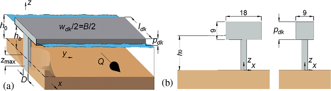
Figure 1: Experimental model (a) 3D view and (b) Longitudinal adopted from [1]

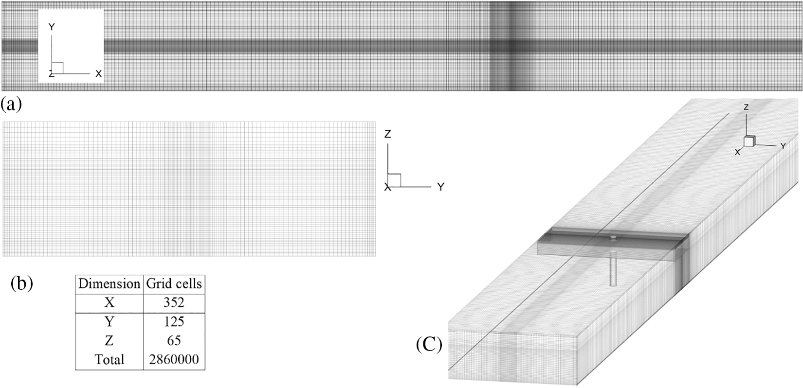
Figure 2: (a) Mesh domain and boundary conditions in (a) Longitudinal plane, (b) Transverse plane, and (c) 3D view along with grid cells in each direction

2.4 Model Verification

The implicit generalized minimal residual method (GMRES) with 120 internal iterations in each step, a 1E-6 initial time step, and the fractional area-volume obstacle representation (FAVOR) method for estimating the free surface were used to estimate the momentum and pressure fields. The model was validated using experimental data from [1]. The turbulent structure of the flow is simulated using smagorinsky’s Large Eddy simulation model (LES). Simulations continued until the results were converged and steady with the stability criteria of velocity variations in 100 consecutive time steps below 0.2%. After then, the simulations are run for an additional 60 s to give enough time steps for the time-averaging procedure. The Assessment of the accuracy of the simulated results is carried out based on a comparison of the stream-wise component of velocity (U) and Turbulent kinetic Energy (TKE) estimated using the computational fluid dynamics (CFD) code to experimental data demonstrates that the numerical results of the velocity Fig. 3 with R2 = 0.941 and TKE with R2 = 0.928 Fig. 4 are in fair agreement with the experimental data.

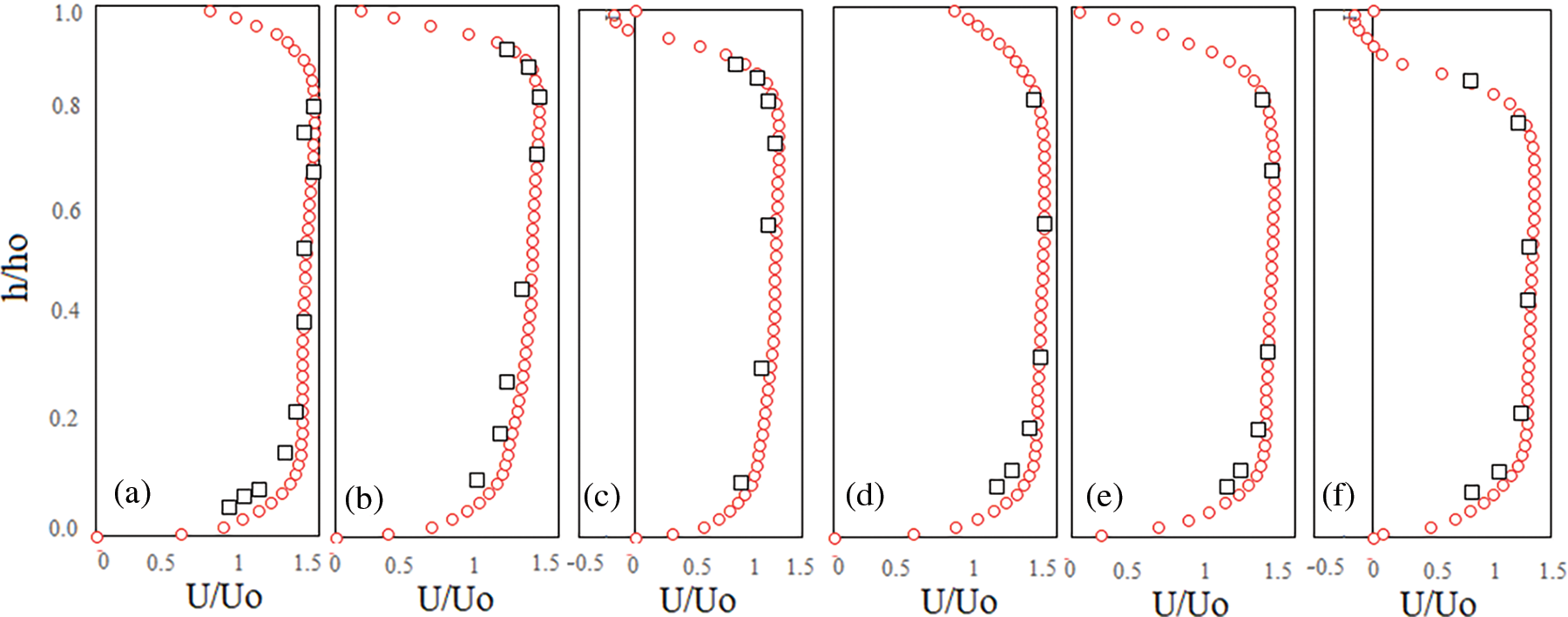
Figure 3: Comparison of experimental and numerical velocity profile of U for Ld/p = 3 at (a) y = 0.65 p, (b) 1.5 p, and (c) 5 p, and Ld/p = 6 (d) y = 0.65 p, (e) 1.5 p, and (f) 5 p

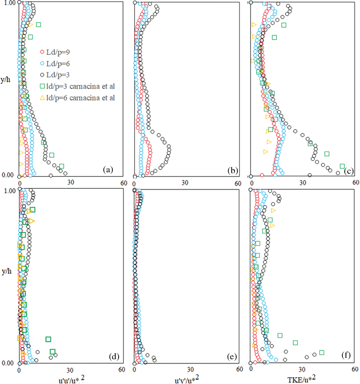
Figure 4: Turbulence intensity parameters at two different verticals (a–c) y/Dp = 0.833 and (d–f) for y/Dp = 1.5 for different dike width ratios compared with experimental results of [1]

Considering the effect of turbulent characteristics of flow on the scouring process, Reynolds stress values of u′v′, u′u′, and Turbulent kinetic Energy (TKE) normalized by the shear velocity values are presented and discussed in Fig. 4. Reynolds stresses depict the turbulence momentum exchange between flow layers and are an indicator of the flow's ability to entrain and transport sediments. Comparing the values, it is indicated that the intensity of turbulent values at case Ld/p = 3 is significantly higher than that of other cases for both upper regions (beneath the deck) and lower regions (channel bed) due to the shorter distance of deck edge from measurement location, which is in agreement with [1] (see Figs. 4a–4b, 4d–4e). Figs. 4c & 4f presents turbulent kinetic energy values at determined verticals. TKE represents the total turbulent intensity of the flow and is calculated as follows:

TKE=(u′2+v′2+w′2)2(5)

It is again clear that the total values of turbulent intensity for Ld/p = 3 are higher than that of other cases, and it reduces as the distance from the pier increases. Besides, compared to u′u′and u′v′, TKE is more affected in mid-depth levels mainly due to the turbulent intensity of the normal component of velocity, and by increasing the distance from the pier, TKE values are reduced.

2.5 Simulation Scenarios

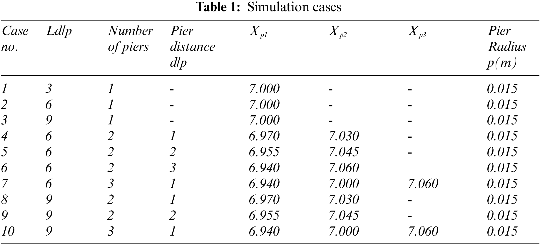
Ten cases are simulated with different geometrical conditions that are shown in Table 1 for each case. Since various research has shown that the length of the bridge deck (Ld) normal to the flow is of inherent importance [1], three different deck lengths of 9, 18, and 27 cm normal to flow are considered to represent the ratio of deck length to pier diameter of Ld/p = 3, 6, and 9. Besides, various studies have also stated that pier arrangement is a dominant factor, heavily affecting flow behaviour. Accordingly, different arrangements of piers with 1, 2, and 3 piers are studied with varying distances between tandem piers. Thus, the impact of the relative deck length Ld/p, the effect of the number of piers and finally, the effect of pier spacing on the flow structure is investigated. The impact of the previously discussed characteristics on the distribution of shear stress along the channel, close to the piers, is then discussed.

3  ML Algorithms

3.1 Decision Trees

Decision trees introduced by [27] are a class of supervised learning algorithms and a good example of a universal function approximator. However, this universality is challenging to attain in its basic form. They could be used for both Classification and regression tasks. Multiple branches, connected by decision nodes and ending in leaf nodes, make up a Decision Tree (DT). With each branch corresponding to an algorithmic choice, the tree's decision node has many possible leaf nodes that reflect model output. For classification or regression, this might be a label, or it could be a continuous value.

3.2 Random Forest Regression

An RFR approach is a machine learning-based regression technique. Using bagging and random subspace as a starting point, it’s a solid basis to build on. Bagging is used to generate a number of learner trees, which are then combined to get an overall prediction. To train the learning trees, bootstrap samples are prepared from the original training data. The initial training data D contains N instances, and each bootstrap sample (Db) is generated by randomly selecting n examples from D. The bootstrap samples may be replaced with new examples. In general, Db is around two-thirds the size of D and has no identical instances. For each of the bootstrap samples, k separate regression trees are built using the input vector, x. Low bias and large variance define the regression trees. Random forest predictions are then produced using the mean forecast of the K regression trees trained on the dataset.

3.3 Adaboost

Boosting is an approach that uses a sequential additive model to create a strong learner by combining a group of weak learners, mainly DTs [28]. The prior model's mistakes are taken into account in the new model, which may be done in various ways. AdaBoost, introduced by [29], is a popular adaptive boosting technique which works by increasing the weight of observations that have been incorrectly estimated in the past. In theory, this might result in a high degree of accuracy.

3.4 Stacked Regression

Stacking regressions, first presented by [24], is a technique for combining many predictors linearly to enhance prediction accuracy. The algorithm mainly consists of two steps of (i) specifying a list of base learners and training each on the dataset and (ii) using the predictions of the base learners as input to train the value of the meta-learner and predict new values with the meta-learner.

3.5 Feed Forward Neural Networks (FFNN)

An FFNN is an artificial neural network based on using neurons as basic constructing elements. These neurons function in such a way to mimic a brain to learn superficial relationships between input-output pairs of information. These algorithms learn by multiplying inputs into weights in each connection and pass the results through an activation function, mostly nonlinear such as Sigmoid, Tanh, and ReLu. This process provides the required nonlinearity to generalize the learning relationship between input and output data. Multi-layer perceptrons (MLPs) are the simplest of the mentioned algorithms, which combine many neurons in parallel structures to learn the data relationships. Further layers could be added to the simple one-layer structure to increase the system's nonlinearity and complexity [28].

3.6 Hyperparameter Optimization

A bayesian optimization is a robust approach for determining the extreme values of computationally difficult-to-solve functions [26]. It may also be used to compute functions that are difficult to calculate, have complicated derivatives to analyze, or are not convex. Bayesian optimization assumes using prior knowledge to find where the function f(x) is minimized according to a criterion by integrating the prior function f(x)′ distribution with the sample information. The function u, known as the acquisition function and represents the criterion, is utilized to calculate the next sample point to maximize anticipated utility. To reduce the number of samplings, it is mandatory to consider both areas with high uncertainty (exploration) and search areas with high values (exploitation), which improves the accuracy as well [30]. Bayesian optimization mainly relies on the previous distribution of the function f, which is not necessarily dependent on the objective criteria but could be based on subjective judgments in part or entirely. The prior distribution of Bayesian optimization is commonly thought to be well-matched to the Gaussian process. Because the Gaussian process is versatile and simple, Bayesian optimization uses it to fit data and update the posterior distribution [30]. For implementation, the Bayes Search CV of scikitopt library [31] for optimization of tree based models, and Keras tuner library [32] for the optimization of MLP model were used.

4  Results and Discussion

4.1 Flow and Turbulence Field

4.1.1 Effect of Deck Width

Fig. 5 shows the streamlines along with the distribution of the U component of velocity at the transverse half-plane at (a, d, g) pier section, (b, e, h) at the end of the bridge deck and (c, f, i) at X = Ld downstream of the pier for different Dike width to pier diameter (Ld/p) ratios (cases no. 1 to 3). The presented velocity field is in agreement with [1,9], and it is indicated that the highest value of the stream-wise component of velocity (U) occurs close to the pier, and the logarithmic velocity profile develops as the distance from the pier increases. As discussed by different researchers, the maximum velocity of the flow occurs at the middle of the channel depth, where maximum velocity forms in the case with Ld/p = 6. Yet, the maximum velocity at Ld/p = 3 occurs closer to the deck (see Figs. 6a, 6b) compared to other cases reported in [1]. Besides, higher velocity gradients are visible in pressurized flow compared to free surface flows [1]. Comparing the streamlines, it could be concluded that two main recirculation areas generally form at the transverse plane at the pier section. The first is a flow separation zone beneath the deck due to the pressure flow effect, and the second is a spiral vortex tangent to the channel side wall. It could be inferred that the height and power of the recirculation zone beneath the bridge deck which is formed due to the downward movement of contour lines by colliding the deck, has increased by increasing the Ld/p ratio from 3 to 6 but reduced with further increase of Ld/p up to 9. Besides, the area of the spiral vortex the channel bottom edge, has constantly increased by increasing the Ld/p and is also detached from the bed in case Ld/p = 9. The size of the spiral vortex at the edge of the channel is increased by increasing the bridge deck length with the largest vortex related to the Ld/p = 9 case. The flow structure at the bridge deck's end for different Ld/p ratios are compared in Figs. 5b, 5e, 5h. It is clear that a complex flow feature forms at the outlet of the pressurized section caused by the bridge deck. The area of the spiral vortex at the edge of the channel for all cases increases compared to the pier section. It is also clear that the maximum value belonging to the case with Ld/p = 9 is slightly larger than that of Ld/p = 6. Generally, the flow structure at the pressurized section outlet in case Ld/p = 6 is more complex compared to other cases. Two counter-rotating vortices formed close to the surface, and a vortex is visible at the channel centre line, which is also larger than that of other cases. Flow at the downstream sections at a distance of Ld/p for each case is depicted in Figs. 5c, 5f, 5i. It is clear that large counter-rotating pairs of surface rollers are formed downstream of the deck section at each side of the pier along with horseshoe vortices which grow and disappear as the flow moves downstream. It should be mentioned that the distance between downstream sections and bridge deck for cases Ld/p = 3 and 6 are smaller compared to Ld/p = 9, which is the reason for reduced velocity and weaker vortices compared to other cases.

Figure 5: Transverse distribution of the U velocity component at different transverse sections for (a–c) Ld/p = 3, (d–f) Ld/p = 6 and (g–i) Ld/p = 9

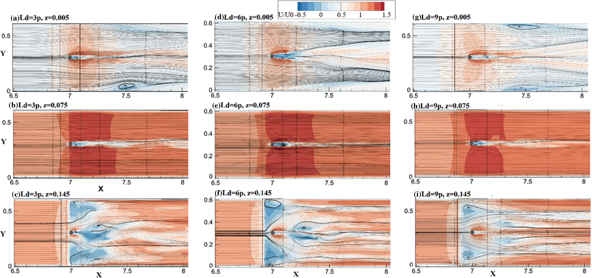
Figure 6: Effect of Ld variations on U velocity distribution in different flow depth

Fig. 6 presents the streamlines and the distribution of U velocity at the x-y plane for three different flow depths, including y/h = 0.03 (5 mm above the bed), y/h = 0.45 and y/h = 0.853 (5 mm beneath the deck). Considering the flow field near the bed for different Ld/p ratios (see Figs. 5a, 5d, 5g), it is clear that the area of the wake vortex behind the pier has increased by increasing Ld/p from 3 to 6 and decreased by a further increase in deck width. Besides, at Ld/p = 6 & 9, clear separation plates are visible, suggesting the formation of spiral flow movements at channel sides.

Considering Figs. 6c, 6f, 6i, it could be inferred that the flow field beneath the deck becomes more uniform as the deck width increase. Thus, by increasing the deck width, the area of the surface rollers downstream of the deck and separation zones beneath the deck decreases. The effect of the Ld/p ratio on flow structure at the x-z plane is depicted in Fig. 7 for two different planes of i) channel centre line (CL) and the second plane with a short distance from the pier (y = 0.285). It is clearly indicated that the area and complexity of the surface roller have decreased as the Ld/p increased from 3 to 6 and almost vanished by a further increase of Ld/p to 9. Besides, the area of the wake vortex behind the bridge pier increases Ld/P from 3 to 6 and decreases at Ld/p = 9.

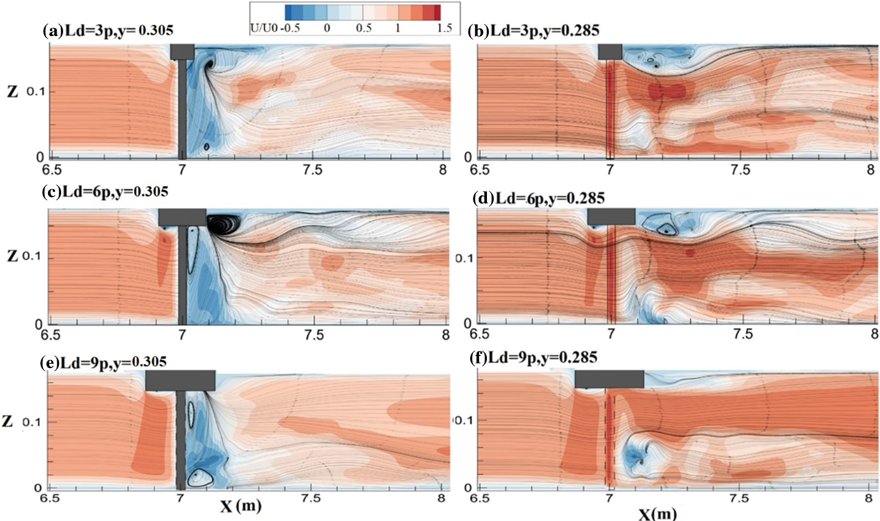
Figure 7: Effect of Ld variations on U velocity distribution in different longitudinal planes

Fig. 8 presents the mean velocity components of U, V, and W for four verticals of (a–c) y/Dp = 0.833 and (d–e) for y/Dp = 1.5 at pier section and at the centre line of the channel, at the beginning of the bridge deck (g–i), and at the end section of bridge deck (j–l) for different dike width ratios. As discussed before, unlike free surface flows, maximum stream-wise velocity occurs around the channel's mid-depth, such as in Ld/P = 6 and 9. Two important features are (1) maximum velocity for Ld/p = 3 occurs closer to the deck, and the maximum value of velocity is almost equal to that of Ld/p = 9; and (2) the maximum value of velocity in case Ld/p = 6 is larger than that for Ld/P = 9. Thus increasing the relative deck width from 3 to 6 has resulted in a slight increase in velocity magnitude due to the increase in the height of the separation zone beneath the deck, which constraints the flow passage area. Yet, a further increase in Ld/p up to 9 has resulted in a reduced height separation zone, larger flow passage area, and consequently smaller velocity than other cases. Considering the distribution of V velocity along the flow depth Figs. 8b & 8e, it is clear that the maximum values occur close to the bed and the deck bottom. Also, it is noticeable that the maximum values of V close to the bed in both y/Dp verticals occur in Ld/p = 6, but the maximum value of V close to the deck bottom occurs in the case with Ld/p = 3. The distribution of the vertical component of velocity (W) is depicted in Figs. 8c & 8f. Considering the higher magnitude of negative W values close to the bed in the case of Ld/p = 3 and higher positive values of case Ld/p = 6, it could be inferred that the horseshoe vortices near the bed are stronger in the case of Ld/p = 3 compared to other deck width rations, while a stronger and thicker flow separation zone formed beneath the deck in case Ld/p = 6 compared to other cases. The vertical profile of velocity at the centre line of the channel at the beginning and final section of the bridge deck is depicted in Figs. 8g–8l. It is indicated that the maximum downward velocity (W) equal to w/U0 = 0.51 occurs at the beginning of the deck for case Ld/p = 6, and the minimum values belong to the case with Ld/p = 3 with w/U0 = 0.38. However, at flow heights close to the bed, the absolute value of w for Ld/p = 3 is slightly larger and increases sharper than that for other cases suggesting higher gradients close to the bed for this case (Fig. 8i). The maximum value of stream-wise velocity for case Ld/p = 3 at the upstream edge of the deck is up to 7% smaller than that of Ld/P = 9 and 6, which is a direct consequence of the smaller distance o flow with the bridge pier (see Fig. 8g). Considering the stream-wise component of velocity (U) a the downstream edge of the deck, it is clear that the recirculation area has spread through the pressurized section outlet with higher absolute values for Ld/p = 9 and decreasing as the deck length decreases. As stated before, increasing the deck length results in the reduction of the area and strength of recirculation zone close to the bed (Fig. 8j). Fig. 8k indicates that the transverse component of velocity close to the bridge deck is higher for Ld/p = 3 and reduces as the deck length increases while a reverse trend is visible close to the bed. It is also indicated that the maximum negative-w is formed in case Ld/p = 6 and 3 suggesting a downward flow movement near the flow surface at the downstream edge of the deck which is related to the formation and disappearance of the surface rollers behind the bridge deck in different length of the deck (see Fig. 6).

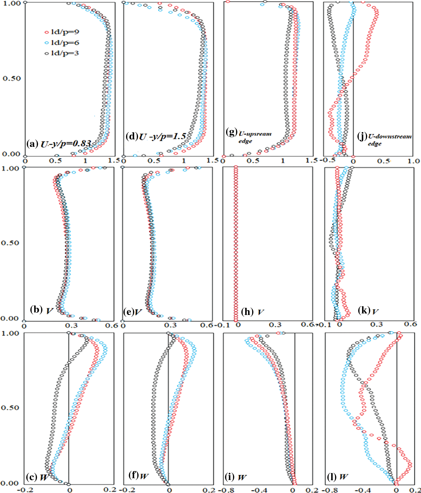
Figure 8: Velocity distribution at two different verticals at the pier section for (a–c) y/Dp = 0.833, (d–f) y/Dp = 1.5, at channel centre line (g–i) at the beginning of deck, and (j–l) at the end of the bridge deck

4.1.2 Effect of Pier Spacing

It is clear that changing the distance between consecutive piers significantly affects the flow structure and scouring intensity. This section studies the effect of increasing the space between consecutive piers in case Ld/p = 6 and two piers with spacing rations of d/p = 1, 2, and 3. Fig. 9 presents the distribution of the stream-wise component of velocity and streamlines at both the x-z and x-y planes. Comparing the maximum velocity and the area of surface roller behind the bridge deck, it could be inferred that despite reducing the distance of the first pier from the deck edge, which might result in an increased turbulence intensity, the maximum values and gradient of velocity in case of d/p = 1 is higher than that for d/p = 2, and 3. Thus it is clear that increasing the distance between consecutive piers may result in the reduction of velocity magnitude and bed shear stress, which in turn suggests a reduced scour intensity. Considering Figs. 9c, 9f, 9i it could be inferred that increasing the space between piers has resulted in a reduction in the area and thickness of the top separation zone while it has significantly increased the area of the downstream surface roller and recirculation area behind the bridge deck.

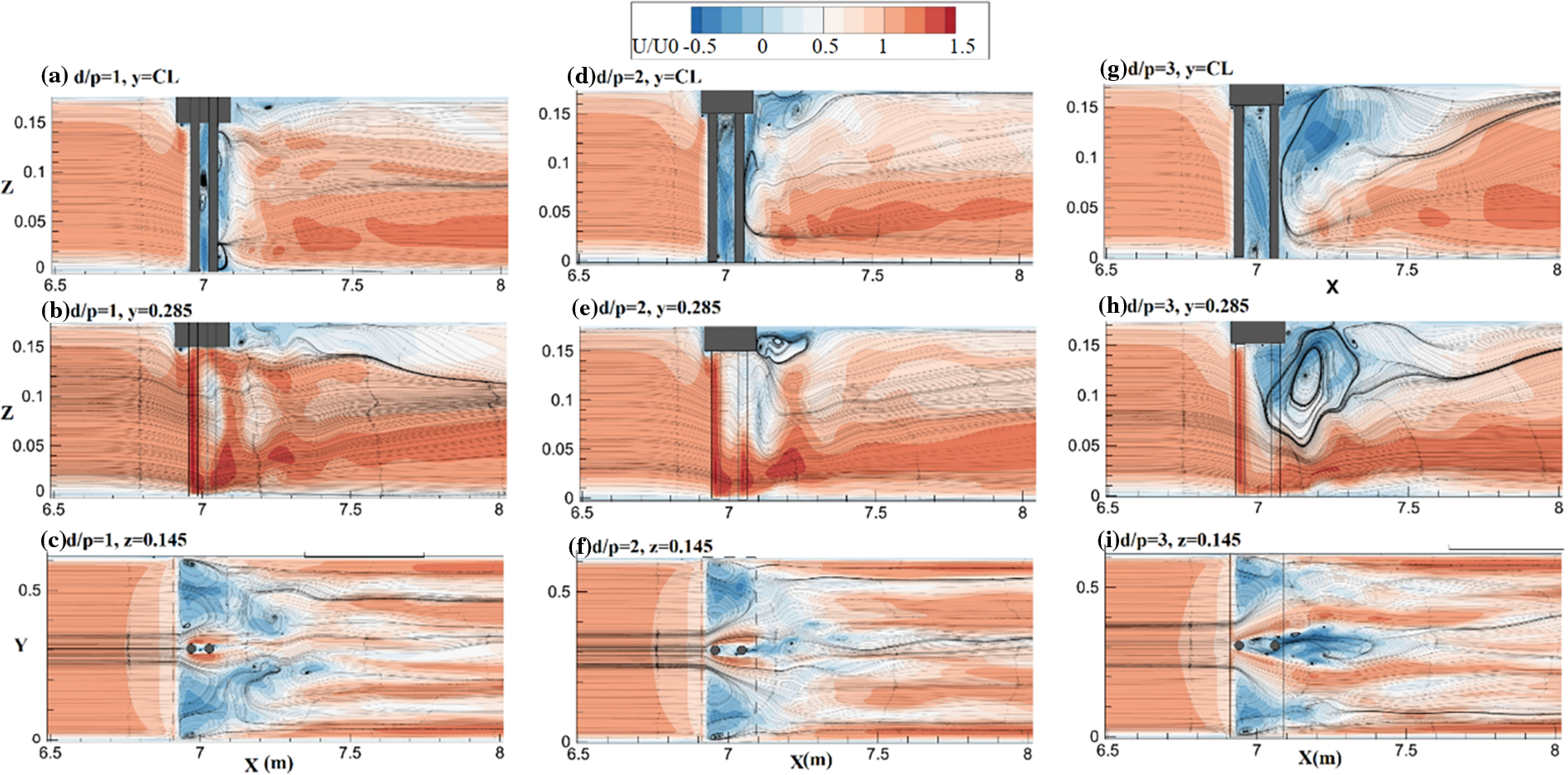
Figure 9: Distribution of stream-wise component of velocity for Ld/p = 6 and different spacing ratios

4.1.3 Effect of Number of Piers

The distribution of stream-wise (U), normal (W) and transverse (V) components of velocity at the centerline of the channel for case Ld/p = 9 and the number of piers equal to 1, 2, and 3 is presented in Figs. 10a–10i. Generally, increasing the number of piers would reduce the distance between the first pier and the deck edge, which may result in increased turbulence intensity at the first pier face. On the other hand, increasing the number of piers could result in an increased flow velocity due to the growth of the recirculation zones behind piers and the decline in the efficient flow passage area. A plan view of the U distribution in different cases is presented in Figs. 10j–10l which suggests that increasing the number of piers has resulted in a significant increase in the area and height of the flow separation zone beneath the deck and the surface roller behind the deck pushing the maximum velocity point towards channel bed.

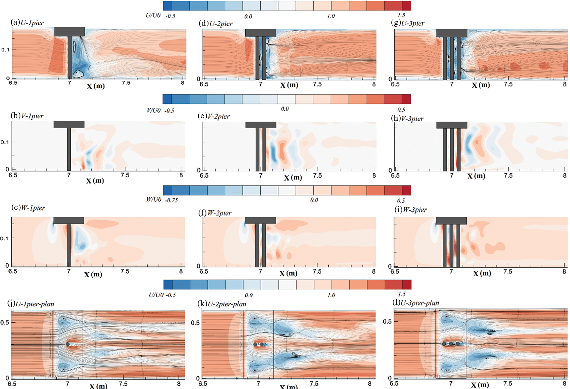
Figure 10: Distribution of U, V and W components of velocity for different pier arrangements and Ld/p = 9

4.2 Shear Stress Distribution

The distribution of Shear stress around bridge piers in cases no. 1 to no. 3 is presented in Fig. 11. It is indicated that the maximum values of shear stress belong to the case with Ld/p = 6. Besides, the area which is affected by high shear stress values in case Ld/p = 6 is larger and wider than that of Ld/p = 3 and 9 suggests that the scour hole in Ld/p = 9 could be wider and deeper than other Ld/p ratios. Yet longer scour hole in Ld/p = 9 would be expected.

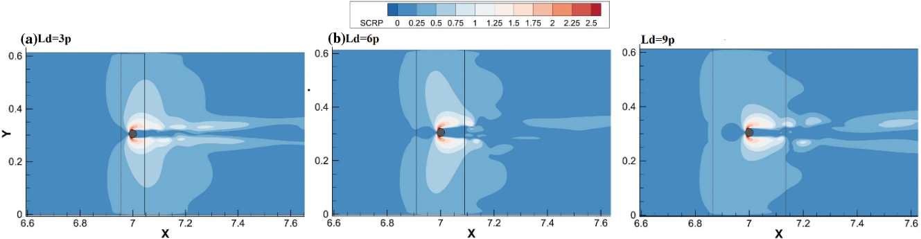
Figure 11: Bed shear stress distribution for different Ld/p values

Fig. 12 presents the distribution of Shear stress tangent to the bridge piers along the x direction in different cases. As discussed above, Figs. 12a & 12b indicates that the values of Shear stress along the channel contraction adjacent to the piers in Case with Ld/p = 6 are larger than that of both Ld/p = 3 and 9 in both longitudinal and transverse planes. The effect of the pier distance on bed shear stress distribution is presented in Fig. 12c. It is indicated that in cases with two tandem piers, increasing the pier distance from d/p = 1 to d/p = 3 results in the reduction of bed shear stress by 17% suggesting that an increase in the pier distance reduces the scour depth, which is different from that for free surface flows reported in [33]. Besides, it should be noted that the maximum value of bed shear stress close to the second pier for d/p = 2 is higher than d/p = 1 and d/p = 3 by 36% and 19%, respectively. Fig. 12d shows that this trend is also valid in the case with Ld/p = 9. In addition, the maximum value of bed shear stress around the first and second piers in tandem formation in Ld/p = 6 is higher than the corresponding values for Ld/p = 9 by 12% and 46% respectively. Fig. 12e compares the bed shear stress values in cases with three piers. It is indicated that the shear stress in cases with Ld/p = 6 for all piers is higher than in cases with Ld/p = 9. The effect of the number of piers on the distribution of shear stress is presented in Fig. 12f. It is indicated that increasing the number of piers from one to two has significantly increased the shear stress values around the first pier by 24%, which may result in an increased scour depth and area for two piers compared to one pier in agreement with open channel flow conditions. Yet, adding the third pier has resulted in a drop in shear stress values by 4% compared to two pier case, suggesting that the maximum depth of scouring for two piers would be slightly higher than that for three pier case.

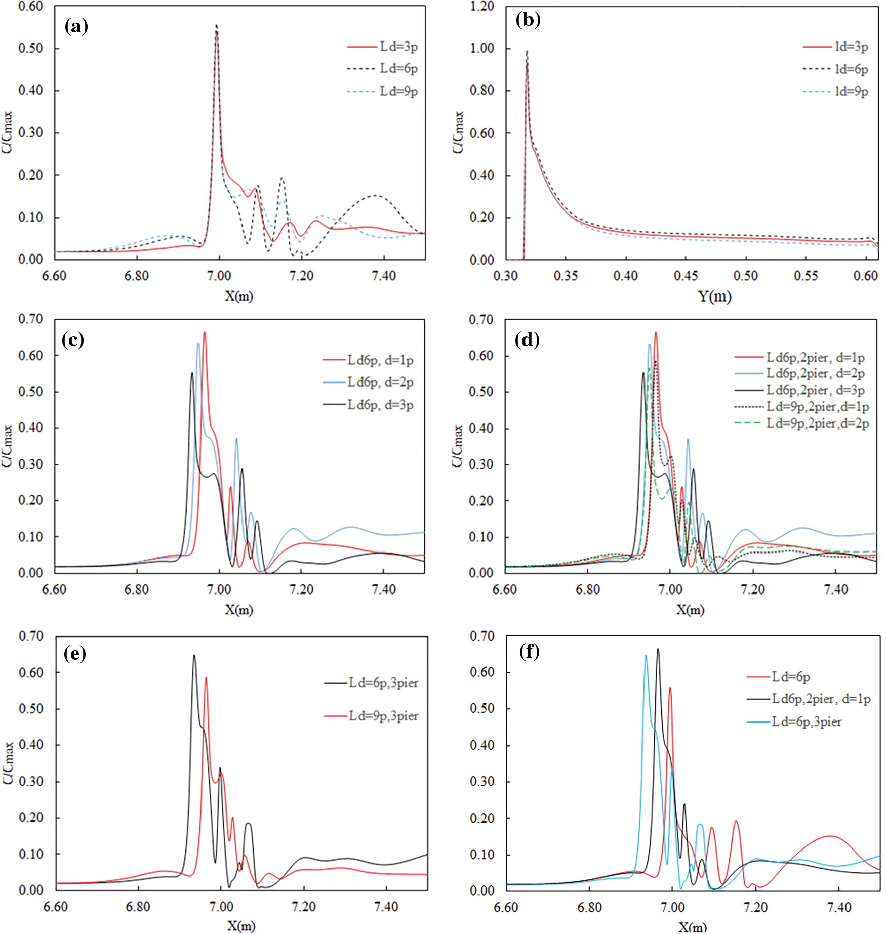
Figure 12: Distribution of bed Shear stress at y = 0.65 p from the center line along bridge piers in x direction (a, c, d, e) and along channel width (b)

4.3 ML Implementation for Flow Field Estimation

As described before, Four Machine learning (ML) algorithms, including Decision Trees and three ensemble models, were implemented to estimate the flow velocity and turbulent field and are compared to a conventional multi-layer perceptron (MLP) network. All models are developed and implemented using Scikit-learn (DT, AdaB, and RF) [34], Mlxtend [35] (Stacked reg.), and Keras (MLP) [36] libraries in python.

4.3.1 Accuracy Assessment

In this paper, three accuracy metrics are used to assess the accuracy of the utilized ensemble models. Accuracy metrics include Mean Absolute error (MAE) Eq. (7):

MAE=∑i=1n|yi−y^i|n(7)

Mean squared error (MSE) Eq. (8):

MSE=∑i=1n(yi−y^i)2n(8)

And the correlation coefficient (R2) Eq. (9):

R2=1−∑i=1n(yi−y^i)2∑i=1n(yi−y¯i)2(9)

where yi is the target values from simulations, y^i is the model predictions, and y¯ represents the mean values.

4.3.2 Dataset Preparation

As discussed above, the dataset includes 10 CFD simulations, of which 8 cases are opted as training and 2 cases, including case no.5 and case no.9, for the test. Values of velocity components within both train and test datasets are normalized between 0 and 1 using maximum and minimum values.

Velocity components, including U, V, W, and Turbulent Kinetic Energy (TKE) output from the CFD model, are considered target values. Input data include the number of piers, the location of each pier at X direction (start and end coordinates), Ld/p ratio for each case, start and end x of bridge dike, y of piers centre, the diameter of piers, and x, y, and z coordinates for each point. Thus, each point in the 3D space has seventeen features with four target values. Considering the complexity of feature space and the varying effect of various feature combinations on the model stability and accuracy, an automatic feature extraction algorithm was utilized. AutoEncoders first introduced by [37] are generally neural networks with a symmetrical structure which could be used to find a better representation of the original data to be learned by the desired machine learning algorithm [38]. In this paper, an Encoder-Decoder model with 34 neurons in the hidden layer and 8 neurons in latent space (Bottleneck) was utilized to map the features into an 8-dimensional space. Encoded data is then used as input data for implemented ML models. The whole procedure resulted in almost 0.8% improvement in the R2 score of U and 0.6% improvement for TKE estimations compared to the models without automatic feature extraction.

4.3.3 Model Results

The Bayesian optimization approach was employed to fine-tune the hyperparameters as they substantially impact the accuracy of the results. The best models were rebuilt and trained over the train-test dataset using a 5-fold Cross-validation. The best model parameters are presented in Table 2. The complete procedure for data preparation and model training is depicted in Fig. 13.

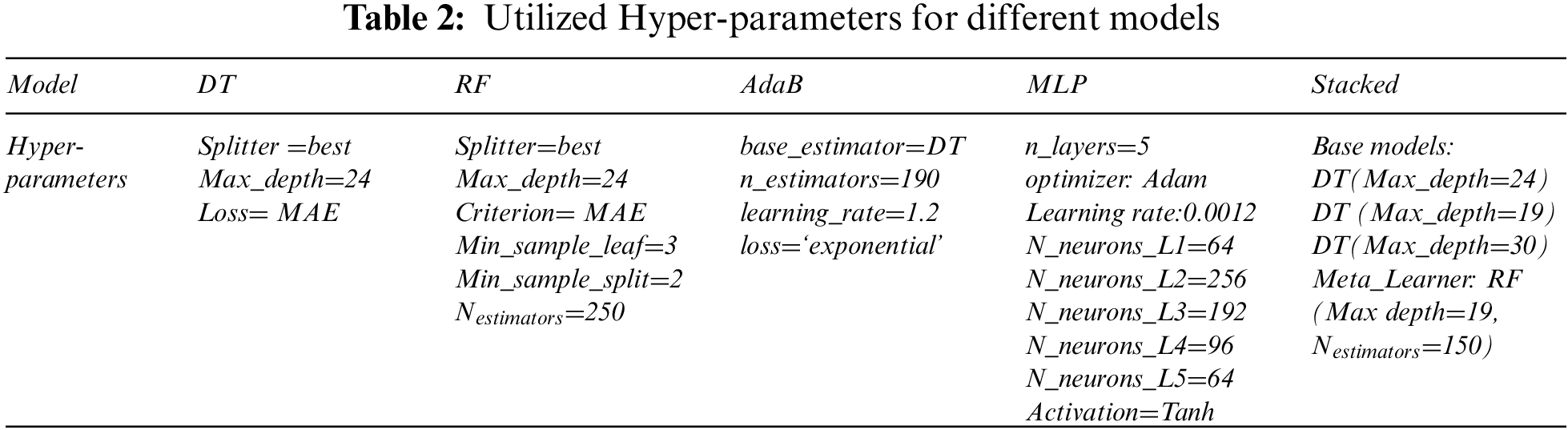
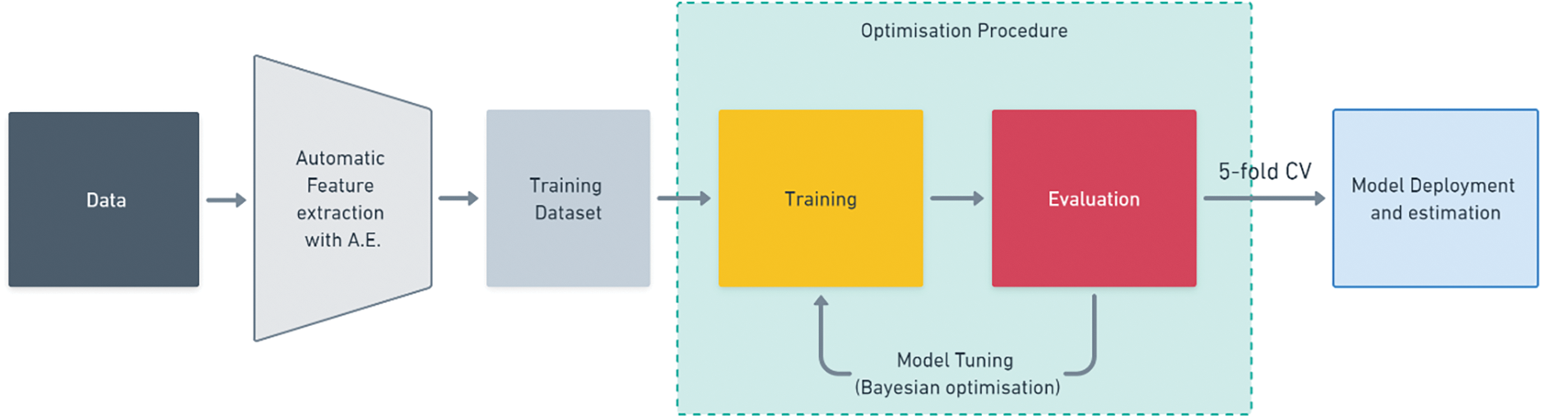
Figure 13: Model training workflow

The performance of different models on the test data set is assessed using the above mentioned accuracy metrics. Obtained values are presented in Table 3 and Fig. 14. Results from the ML algorithms indicate that the general accuracy of the Turbulent Kinetic Energy (TKE) estimations is higher than the Velocity vectors. Besides, the lowest estimations accuracy belongs to all models’ V- velocity components.

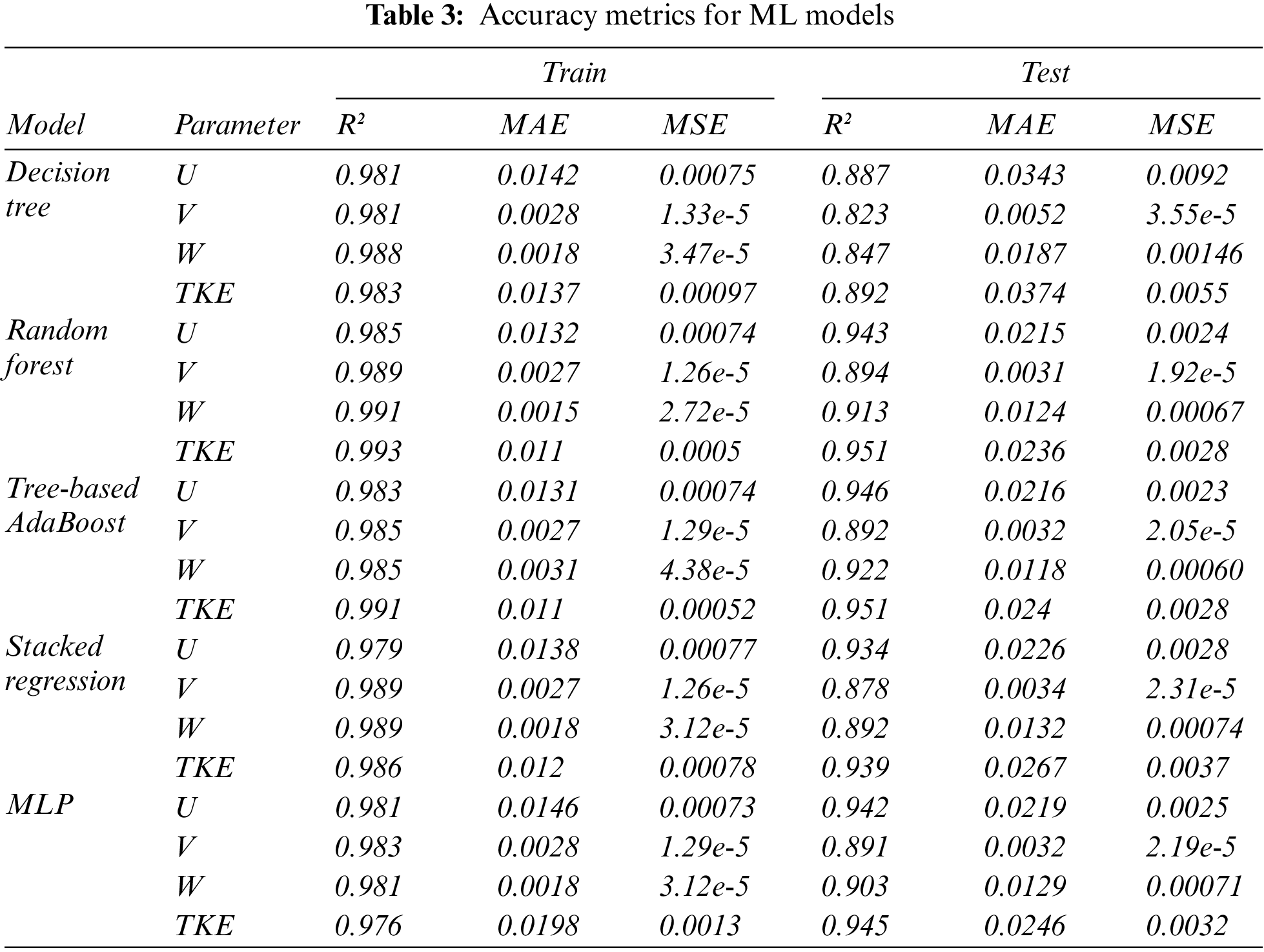
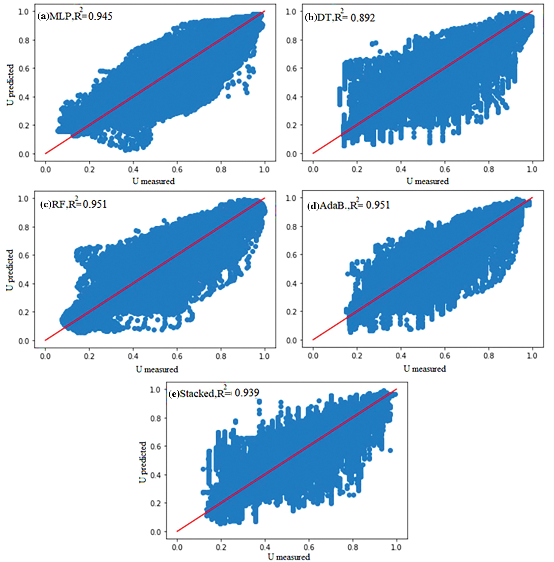
Figure 14: Estimations of Turbulent kinetic Energy for different ML models vs CFD results

Generally, it is indicated that using Ensemble models has increased the accuracy compared to the base Decision Tree Regression or MLP model. Random Forest showed the best performance among other models with R2= 0.899 for V-velocity estimation. AdaBoost slightly outperformed other models in the estimation of U, W, and TKE. The stacked model has presented slightly weaker results than other ensemble models, and MLP since as the difference between results of the base learners (decision tree) decreases, the stacked regression accuracy would also reduce. This algorithm is most efficient when combining different algorithms, mainly deep or ensemble models as base models. Yet, in this research, the base and meta-learners are set to be Decision trees and random forest, making the model less efficient.

Considering the fact that simulated cases have indicated significant variations in velocity distribution in different cases, it could be concluded that training a proper ML algorithm on eight simulations and estimating two other cases might not result in an appropriate surrogate for the CFD for operational use in the current case of studies. However, estimations of the TKE and U-velocity have acceptable accuracies, yet, the majority of errors arise from the areas close to the piers, including the horseshoe vortices, recirculation zone and the flow separation areas beneath the bridge deck. Besides, it should be noted that the error of the estimation of the Case no.9 is generally higher than that for Case no.5 by 3.5%. It could be noted that, due to the fact that scenarios with Ld/p = 9 include only two simulations with two piers, including cases no. 8 and 9, trying to estimate Case no. 9 is more similar to extrapolation for the model rather than an interpolation resulting in the lower accuracy compared to case 5 and reducing the overall accuracy of the trained models.

On the other hand, Comparing the estimated values for different flow depths shows that the accuracy of the estimations is the most for z = 0.005, in which the flow perturbation is minimal. By moving towards the surface (and the deck bottom), the accuracy of results decreases to the minimum values at h/h = 0.97 (z = 0.145 m), where the flow perturbation and recirculation zones are the dominant flow patterns. For example, the accuracy of estimations for the stream-wise component of velocity (U) provided by the Random Forest at h/h0 = 0.34 (close to the bed) is equal to R2 = 0.956, at h/h0 = 0.5 is R2 = 0.934, and at h/h0 = 0.97 is minimum and equal to R2 = 0.874. For the MLP model, R2 values for mentioned flow depth are equal to 0.958, 0.932, and 0.871, respectively. However, the mentioned values for Adaboost regression model are equal to R2 = 0.959, 0.937, and 0.865 for h/h0 = 0.34, 0.5, and 0.97 respectively. Consequently, it is indicated that even though the overall accuracy of the estimations is limited due to the limitations in simulation scenarios and training cases, yet, the implementation of ensemble models has been effective in increasing accuracy, especially for flow zones close to the deck bottom (h/h0 = 0.97) such as increasing the U estimation accuracy from R2 = 0.798 of Dt model to R2 = 0.874 for AdaBoost model. Hence, utilizing Ensemble models with sufficient training cases could result in proper surrogates.

5  Conclusion

Failure of bridges due to the pier scour is an important phenomenon which intensifies in pressurized flow conditions. A thorough analysis of the stream’s flow patterns and turbulent behaviour is required in order to comprehend the scour process completely. This article aims to examine the interaction between deck width, the number of bridge piers, and the distance between adjacent piers in a tandem arrangement. Hence, the total number of 10 simulations with three different deck width to pier diameter ratios (Ld/p) of 3, 6, and 9 are performed with different combinations of 1, 2 and 3 circular bridge piers. Results indicate that by increasing the width of the deck-to-pier ratio, the area of maximum flow velocity moves from near the deck bottom toward the mid-depth of the channel. Besides, the area of the flow separation zone beneath the deck increases by increasing the Ld/p up to 6, yet it decreases by a further increase of Ld/p to 9. Besides, a surface roller forms behind the deck, which is weakened by increasing the deck width to 9, where it has the minimum area and power. Comparing velocity and turbulent kinetic energy magnitudes, it could be inferred that the turbulent fluctuations and near bed vortices in case Ld/p = 3 are stronger than that for other Ld/p ratios. Besides, increasing the number of piers results in a smaller distance from the deck edge to the pier, increasing turbulence around the pier and increasing the separation zone area beneath the deck and surface rollers behind the deck. It was also found that the bed shear stress around the piers is maximum in two pier formations, with values about 2% and 9% higher than that for three pier and one pier formations, respectively. Consequently, it could be inferred that the maximum scour depth would be higher in cases with two piers compared to the single-pier and triple pier formations. In addition, Increasing the distance between consecutive piers would result in decreased values of maximum velocity and bed shear stress.

In the second part, five different machine learning models, including Decision Tree, Random Forest, AdaBoost regressor, Stacked Regression, and Multi-layer perceptron (MLP), are implemented in combination with automatic feature extraction using autoencoders models hyper-parameters optimization using Bayesian to estimate the flow field and turbulent structure of the flow. Results indicated that the ensemble models generally increased the accuracy of estimations compared to base models. The AdaBoost regressor model slightly outperformed other ensembles in the estimation of the velocity and turbulent quantities, with R2= 0.946 for the estimation of U and R2= 0.951 for the estimation of TKE. Besides, the maximum improvement of ensemble models compared to base models is observed to be in areas with higher complexity in which the accuracy of estimations in U and V components of velocity is increased up to 6% and 7%, respectively.

Acknowledgement: The authors gratefully acknowledge the financial support from the National Natural Science Foundation of China (Grant Nos. 52179060 and 51909024).

Funding Statement: This research is financially supported by the National Natural Science Foundation of China (Grant Nos. 52179060 and 51909024).

Conflicts of Interest: The authors declare that they have no conflicts of interest to report regarding the present study.

References

1. I. Carnacina, N. Leonardi and S. Pagliara, “Characteristics of flow structure around cylindrical bridge piers in pressure-flow conditions,” Water, vol. 11, no. 11, pp. 2240, 2019. [Google Scholar]
2. S. E. Gill, J. F. Handley, A. R. Ennos and S. Pauleit, “Adapting cities for climate change: The role of the green infrastructure,” Built Environment, vol. 33, no. 1, pp. 115–133, 2007. [Google Scholar]
3. S. B. Goldenberg, C. W. Landsea, A. M. Mestas-Nuñez and W. M. Gray, “The recent increase in atlantic hurricane activity: Causes and implications,” Science, vol. 293, no. 5529, pp. 474–479, 2001. [Google Scholar]
4. L. Wright, P. Chinowsky, K. Strzepek, R. Jones, R. Streeter et al., “Estimated effects of climate change on flood vulnerability of U.S. Bridges,” Mitigation and Adaptation Strategies for Global Change, vol. 17, no. 8, pp. 939–955, 2012. [Google Scholar]
5. E. R. Umbrell, G. K. Young, S. M. Stein and J. S. Jones, “Clear-water contraction scour under bridges in pressure flow,” Journal of Hydraulic Engineering, vol. 124, no. 2, pp. 236–240, 1998. [Google Scholar]
6. I. Carnacina, S. Pagliara and N. Leonardi, “Bridge pier scour under pressure flow conditions,” River Research and Applications, vol. 35, no. 7, pp. 844–854, 2019. [Google Scholar]
7. M. Fathi-moghaddam, M. T. Sadrabadi and M. Rahmanshahi, “Numerical simulation of the hydraulic performance of triangular and trapezoidal gabion weirs in free flow condition,” Flow Measurement and Instrumentation, vol. 62, pp. 93–104, 2018. [Google Scholar]
8. H. Karami, S. Farzin, M. T. Sadrabadi and H. Moazeni, “Simulation of flow pattern at rectangular lateral intake with different dike and submerged vane scenarios,” Water Science and Engineering, vol. 10, no. 3, pp. 246–255, 2017. [Google Scholar]
9. S. Dey and R. V. Raikar, “Characteristics of horseshoe vortex in developing scour holes at piers,” Journal of Hydraulic Engineering, vol. 133, no. 4, pp. 399–413, 2007. [Google Scholar]
10. C. Manes and M. Brocchini, “Local scour around structures and the phenomenology of turbulence,” Journal of Fluid Mechanics, vol. 779, pp. 309–324, 2015. [Google Scholar]
11. B. W. Melville and A. J. Raudkivi, “Flow characteristics in local scour at bridge piers,” Journal of Hydraulic Research, vol. 15, no. 4, pp. 373–380, 1977. [Google Scholar]
12. D. A. Lyn, “Pressure-flow scour: A reexamination of the hec-18 equation,” Journal of Hydraulic Engineering, vol. 134, no. 7, pp. 1015–1020, 2008. [Google Scholar]
13. L. A. Arneson and S. R. Abt, “Vertical contraction scour at bridges with water flowing under pressure conditions,” Transportation Research Record, vol. 1647, no. 1, pp. 10–17, 1998. [Google Scholar]
14. J. Guo, K. Kerenyi, J. E. Pagan-Ortiz and K. Flora, “Bridge pressure flow scour at clear water threshold condition,” Transactions of Tianjin University, vol. 15, no. 2, pp. 79–94, 2009. [Google Scholar]
15. E. Hahn, Clear-Water Scour at Vertically or Laterally Contracted Bridge Sections. West Lafayette, Indiana, United States: Purdue University: School of Civil Engineering, 2005. [Google Scholar]
16. C. Lin, M. -J. Kao, S. -C. Hsieh, L. -F. Lo and R. V. Raikar, “On the flow structures under a partially inundated bridge deck,” Journal of Mechanics, vol. 28, no. 1, pp. 191–207, 2012. [Google Scholar]
17. K. S. Yoon, S. O. Lee and S. H. Hong, “Time-averaged turbulent velocity flow field through the various bridge contractions during large flooding,” Water, vol. 11, no. 1, pp. 143, 2019. [Google Scholar]
18. L. Sang, J. Wang, T. Cheng, Z. Hou and J. Sui, “Local scour around tandem double piers under an ice cover,” Water, vol. 14, no. 7, pp. 1168, 2022. [Google Scholar]
19. B. Ataie-Ashtiani and A. A. Beheshti, “Experimental investigation of clear-water local scour at pile groups,” Journal of Hydraulic Engineering, vol. 132, no. 10, pp. 1100–1104, 2006. [Google Scholar]
20. J. Fürnkranz, “Decision tree,” In: C. Sammut and G. I. Webb (Eds.Encyclopedia of Machine Learning, pp. 263–267. Boston, MA: Springer US, 2010. https://doi.org/10.1007/978-0-387-30164-8_204. [Google Scholar]
21. G. N., P. Jain, A. Choudhury, P. Dutta, K. Kalita et al., “Random forest regression-based machine learning model for accurate estimation of fluid flow in curved pipes,” Processes, vol. 9, no. 11, pp. 2095, 2021. [Google Scholar]
22. H. Tin Kam, “Random decision forests,” in Proc. of 3rd Int. Conf. on Document Analysis and Recognition, Montreal, QC, Canada, 1995. [Google Scholar]
23. “Adaboost,” In: S. Z. Li and A. Jain (Eds.Encyclopedia of Biometrics, pp. 9. Boston, MA: Springer US, 2009. https://doi.org/10.1007/978-0-387-73003-5_825. [Google Scholar]
24. L. Breiman, “Stacked regressions,” Machine Learning, vol. 24, no. 1, pp. 49–64, 1996. [Google Scholar]
25. S. Haykin, Neural Networks: A Comprehensive Foundation. United States: Prentice Hall PTR, 1994. [Google Scholar]
26. E. Brochu, V. Cora and N. de Freitas, A Tutorial on Bayesian Optimization of Expensive Cost Functions, with Application to Active User Modeling and Hierarchical Reinforcement Learning. University of British Columbia: Department of Computer Science, 2016. [Google Scholar]
27. L. Breiman, J. H. Friedman, R. A. Olshen and C. J. Stone, “Classification and regression trees,” New York, USA: Routledge, pp. 368, 1983. [Google Scholar]
28. P. Jain, S. C. P. Coogan, S. G. Subramanian, M. Crowley, S. Taylor et al., “A review of machine learning applications in wildfire science and management,” Environmental Reviews, vol. 28, no. 4, pp. 478–505, 2020. [Google Scholar]
29. Y. Freund and R. E. Schapire, “A decision-theoretic generalization of on-line learning and an application to boosting,” Journal of Computer and System Sciences, vol. 55, no. 1, pp. 119–139, 1997. [Google Scholar]
30. J. Wu, X. -Y. Chen, H. Zhang, L. -D. Xiong, H. Lei et al., “Hyperparameter optimization for machine learning models based on bayesian optimizationb,” Journal of Electronic Science and Technology, vol. 17, no. 1, pp. 26–40, 2019. [Google Scholar]
31. T. Head, MechCoder, G. Louppe, I. Shcherbatyi, fcharras et al.Scikit-optimize/scikit-optimize: V0.5.2. 2018. [Online]. Available: https://doi.org/10.5281/zenodo.1207017. [Google Scholar]
32. K. Team, Keras documentation: Keras tuner. 2021. [Online]. Available: https://keras.io/keras. (accessed August 24, 2021). [Google Scholar]
33. H. S. Kim, M. Nabi, I. Kimura and Y. Shimizu, “Numerical investigation of local scour at two adjacent cylinders,” Advances in Water Resources, vol. 70, pp. 131–147, 2014. [Google Scholar]
34. F. Pedregosa, G. Varoquaux, A. Gramfort, V. Michel, B. Thirion et al., “Scikit-learn: Machine learning in python,” Journal of Machine Learning Research, vol. 12, pp. 2825–2830, 2011. [Google Scholar]
35. S. Raschka, “Mlxtend: Providing machine learning and data science utilities and extensions to python’s scientific computing stack,” The Journal of Open Source Software, vol. 3, pp. 24, 2018. [Google Scholar]
36. F. O. Chollet, Keras. 2015. [Online]. Available: https://github.com/fchollet/keras. [Google Scholar]
37. D. H. Ballard, “Modular learning in neural networks,” in AAAI, Seattle, Washington, 1987. [Google Scholar]
38. D. Charte, F. Charte, M. J. del Jesus and F. Herrera, “A practical tutorial on autoencoders for nonlinear feature fusion: Taxonomy, models, software and guidelines,” Information Fusion, vol. 44, pp. 78–96, 2018. [Google Scholar]
Cite This Article
Copyright © 2023 The Author(s). Published by Tech Science Press.
This work is licensed under a Creative Commons Attribution 4.0 International License , which permits unrestricted use, distribution, and reproduction in any medium, provided the original work is properly cited.
Downloads
Citation Tools