RankXGB-Based Enterprise Credit Scoring by Electricity Consumption in Edge Computing Environment

1  Introduction

Enterprise credit analysis plays a key role in reducing financial risks, which is important for venture capital [1] and bank loans. It is helpful to determine the loan limit and interest rates of the enterprise. Most existing credit rating methods [2,3] rely on the candidates’ historical operational and financial data. Though these data are highly related to business credit, some enterprises cannot provide complete information. The lack of the borrower’s credit history can increase the financial risks heavily. Recent studies show a close relationship between electricity consumption and the operation state [4–6]. Besides, with the maturity of IoT, enterprise electricity consumption data can be collected accurately at any time. With the accumulation of large-scale enterprise electricity consumption, it is impractical to analyze them manually by financial and energy experts. Thus, it demands a novel way to realize intelligent credit scoring automatically and effectively.

Recently, some methods have used deep learning for credit scoring, which can extract complex structures and effective representations in large-scale business data [7–9]. These methods aim to generate the credit level or judge whether the borrower defaults directly, which is usually a binary class classification problem. Such qualitative prediction result is too simple to satisfy the requirements of the financial institution, such as the amount, the interest rate, and the borrowing period of the loan. Determining these values requires quantitative evaluation of credit degree, rather than binary judgment. Thus, a more effective way is to provide an absolute value to show the credit degree of the enterprise. Such quantitative evaluation is especially important for credit scoring from electricity consumption since it is usually used as a supplementary clue for manual post-process with other business information. For many deep learning applications, the regression method is a natural choice to predict continuous values, such as visibility estimation [10] and facial landmark detection [11].

However, when using deep regression for credit scoring, the complexity of the relationship between electricity consumption data and credit score increases the size of the deep network significantly. To ensure fast response, powerful computing resource is required to execute such a complex deep network. Considering the limited computing resource in edge devices, it is not suitable to deploy the network in the edge device, especially the mobile terminal [12]. In addition, the electricity consumption data of each enterprise is usually scattered and stored in the data centers near the enterprise. The distributed electricity consumption data brings many difficulties to credit evaluation since the score prediction requires a unified standard. To realize data consistency, some methods use cloud computing for credit scoring [13], but the massive computing tasks increase the processing latency of the computing center.

To overcome the challenging problem of cloud computing, this paper proposes to use edge computing to realize enterprise credit scoring from electricity consumption based on deep learning. Edge computing is a computing paradigm to execute some tasks at the edge of the network, which can process and secure the data faster. Compared with cloud computing, the excessive energy consumption of the server can be saved and the pressure of network bandwidth can be reduced. To meet the real-time requirements of credit scoring, our method allocates the computing tasks in the edge terminal and the cloud server. We carry out the deep learning inference tasks in the cloud server. By the distributed computing clusters equipped with the graphics processing unit (GPU) in the cloud server, we improve the execution speed of the deep model. We then use the weak computing resources in the edge device to realize the post-processing operation. Despite the strong computing power in the cloud, the enterprise electricity consumption data is updated frequently, and the latency should be low. Thus, we need to design a special deep model to reduce the computational overhead in the cloud server.

To reduce the network complexity, our method does not create a direct mapping between electricity consumption and credit score. In contrast, the goal of our deep model is to judge which enterprise has a higher credit score among the given two enterprises. Fig. 1 shows the comparison between the regression model and the ranking model. The regression model takes one enterprise’s electricity consumption data as input and outputs its credit score. In contrast, the input of our ranking model is two enterprises, and the output is a judgment of the relative credit. Since such relative judgment is much simpler than the regression task, a network with fewer parameters can be used to achieve satisfactory performance with fewer computing resources. In addition, when constructing the training dataset, users can make more accurate annotations according to local information. In contrast, it is impractical to directly give the credit score manually since it requires knowledge of the global distribution information of the whole training data set. Thus, compared with the annotation of the regression method, our annotation is more accessible and accurate, which leads to an accurate ranking model.

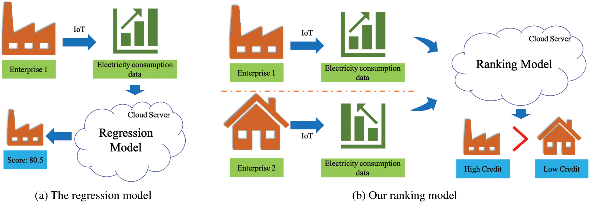
Figure 1: The comparison between the regression model and our ranking model

Inspired by a recent ensemble learning framework [14,15], we propose a novel deep ranking model called rankXGB in an edge computing framework for credit scoring from electricity consumption. Unlike existing ranking methods using only a single model [16], the rankXGB consists of several weak ranking models by using the ranknet as the base model for performance boosting, which is learned successively by the extreme gradient boosting algorithm (XGBoost). These weak ranking models generate several weak ranking results, and the results are then fused to produce a more reliable prediction. To improve the robustness of the rankXGB model, we propose a ranking-based representative enterprise sample selection method to remove some inconsequential samples.

Such a model is very suitable to be deployed in an edge computing environment since the weak ranking models are very lightweight and can be executed in parallel in the cloud server. Besides, the mechanism of model fusion is based on a linear combination, which can be offloaded on the edge terminal to reduce the workload of the cloud server. According to the offload decision, our edge computing framework consists of a two-stage task architecture including a cloud-based weak credit ranking and an edge-based enterprise credit score calculation. It first uploads the electricity consumption data of the evaluated enterprise from the IoT data center to the computing cloud server. Then, during the cloud-based weak credit ranking stage, the cloud server employs its powerful GPU clusters to run the weak ranking models in parallel. This realizes weak credit ranking, which is the weak credit ranking judgments with some predefined benchmark enterprises. Finally, all the credit ranking results are sent back to the edge terminal, where a ranking fusion process and a score normalization are successively executed. The ranking fusion process fuses all the weak credit ranking judgments into a more reliable result, while the score normalization stage produces an absolute credit score of the evaluated enterprise.

To show the effectiveness of our method, we collect a set of enterprises with electricity consumption data captured by the IoT devices. Some financial experts are recruited to remove the unrelated index and label each pair of enterprises in the collected data set. We evaluate our system on the data set and show our method leads to high accuracy and efficiency.

There are three innovations in this method as follows.

1.    We design an edge computing framework to support fast enterprise credit scoring from electricity consumption based on deep learning, which improves the efficiency of large-scale electricity consumption data analysis.

2.    We propose a rankXGB model for enterprise credit evaluation, which improves the performance of the credit ranking by fusing multiple weak ranking models.

3.    We create a benchmark dataset for enterprise credit scoring from electricity consumption, while experimental analysis shows that the proposed method achieves state-of-the-art performance.

2  Related Work

This section reviews the existing research related to the work of this paper, including three sections on credit scoring, learning to rank, and edge computing.

2.1 Credit Scoring

Credit scoring aims to avoid transaction risks, and it is realized by conducting credit evaluations on certain aspects of the enterprise to ensure objective and reliable results. With the development of the social economy, credit scoring can be applied to all aspects of social and economic life [17]. The early researches rely on expert opinions, such as Delphi expert scoring [18]. However, it is usually followed by multiple rounds of adjusted feedback, which is very tedious for the vast of loan applications. To solve it, many artificial intelligence techniques are introduced to realize automatic credit scoring [19]. For example, the hierarchical analysis method treats credit scoring as a multi-objective optimization problem by computing the weight of each indicator [20]. The factor analysis method classifies the variables into several groups to identify hidden representative factors among many variables [21].

Recently, machine learning has become the mainstream technique for credit scoring [22]. Most existing methods consider credit scoring as a binary classification problem, which only judges whether the applicant can successfully get a loan. For example, Liu et al. [23] use two tree-based augmented gradient boosting decision trees (GBDTs) to realize credit management. Liu et al. [24] use multi-grained and multi-layered GBDTs for credit scoring. Li et al. [25] use support vector machine (SVM) to learn a loan evaluation model. West [26] investigates credit scoring by five neural network models. Nowadays, deep learning has become a powerful technique for big data analysis [27], which can learn the feature representation and the classifier in an end-to-end way. The technique is widely used in many applications, such as flooding process prediction [28], visibility estimation [10], shape recognition [29], object detection [30], visual question answering [31], insect pest recognition [32], advertising click-through rate prediction [33], event extraction [34], sneaker recognition [35], modulation recognition [36], sentiment analysis [37], intrusion detection [38–40], climate prediction [41], internet of vehicles [42], healthcare [43], and face clustering [44]. Due to the advantage of deep learning, various researchers apply deep learning to predict credit scores. Babaev et al. [45] employ an embedding transactional recurrent neural network to compute credit scores from transnational data. Wu et al. [46] utilize deep multiple kernel learning to predict credit defaults. Compared with the credit scoring method based on traditional machine learning, deep learning provides a more accurate classification of load applicants. Our method also uses deep learning for credit scoring. Instead of outputting the binary judgment, we produce an absolute credit score to show the risk degree of the enterprise, which is more informative and meaningful for bank loans.

2.2 Learning to Rank

Learning-to-rank framework is initially used for information retrieval, which produces the best order of the item list. According to the type of loss function, existing learning-to-rank methods are divided into three categories: pointwise [47–49], pairwise [50,51], and listwise [52,53]. The pointwise method [47–49] learns a model to assign a suitable score to each item, and the scores of all the items represent the ranking values. Thus, the pointwise method is equal to the regression problem. Compared with the pointwise method, the pairwise method [50,51] cares more about the order between a pair of items, and it mainly reduces the sorting problem to a binary classification problem. The listwise method [52,53] directly optimizes the items’ sorting results concerning the evaluation metrics. In summary, the pointwise method ignores the relationship between samples and treats each sample independently of one another, which cannot generate satisfactory results. The listwise method requires a long list of samples for ranking optimization, but the computational complexity is very high. A common disadvantage of these two methods is that they require full order of all the samples. To avoid these issues, we choose to use pairwise methods for our applications, which realizes the compromise between performance and efficiency. Among existing pairwise methods, we are particularly interested in the ranknet method [50], since it is easy to be integrated into the deep learning framework. Different from the original ranknet method, we improve the performance by adding an XGBoost layer as the last layer of the ranknet model. The XGBoost layer combines several weak ranknet models to achieve a strong ranking model. To the best of our knowledge, this is the first time to combine XGBoost and deep ranknet for performance boosting.

2.3 Edge Computing

Cloud computing employs a central server for various applications by data fusion [54], which brings a high cost to the central server. To solve this problem, edge computing moves some tasks to the edge of the network with some computational capabilities [55–57]. One of the existing edge computing paradigms is mobile edge computing, which provides low-latency services by distributing computing and storage resources to the ends close to the mobile terminal users. To ensure resource efficiency, Xu et al. [58] propose an edge content caching method by service requirement prediction based on the deep spatio-temporal residual network. To minimize the execution time, Chen et al. [59] also use the deep reinforcement learning method [60,61] to realize a distributed computation offloading strategy for intelligent connected vehicles. Another challenging problem is the energy cost, which can be solved by wireless power transfer effectively [62,63]. Nowadays, we can utilize the computing resource of the edge computing environment to train deep learning models for high elasticity. To improve the overall performance of multiple deep learning tasks, Gu et al. [64,65] propose to arrange the job scheduling by considering the data cache and deep learning tasks [66]. Wu et al. [30] utilize the edge computing framework to achieve image enhancement and object detection in a mobile environment efficiently. Edge computing also enriches the paradigms of machine learning. For example, Liu et al. [67] propose an efficient-communication federated learning approach to protect consumer data privacy. Our method also uses edge computing for deep learning-based applications, and we propose a two-stage task architecture, which contains a cloud-based credit score sorting and an edge-based credit score calculation to realize high-through big data analysis.

3  Method

Fig. 2 shows the structure of our edge computing framework. The IoT devices deployed in enterprises collect electricity consumption data at all times. Once the consumption data is collected, it is uploaded to the data center in the cloud environment, which belongs to the grid power company. With the accumulation of the record, the business state can be reflected by the data, resulting in a reliable data resource for credit scoring. When the users want to obtain the credit score of an enterprise, they first send the name of the enterprise to the data center by personal computer (PC) or mobile phone. Then, our system extracts the electricity consumption data related to the credit judgment from the data center and passes the extracted data to the computing server in the cloud. To extract the data, we locate the enterprise and search the nearest data center to query the database by structured query language. All the data has a unique key related to the name of the enterprise. After the data transmission, the computing server performs a weak credit ranking by our pre-trained deep model. Finally, the weak ranking results are transferred to the edge terminal, and the edge device executes the score calculation method to obtain the credit score. It is worth noting that the electricity consumption data involves the privacy of the enterprise. As a result, when the terminal sends the request, it should send a query license certificate signed by the enterprise. To ensure the security of the certificate, we use the ellipse curve cryptography algorithm to generate the certificate, and the certificate is evaluated by the certification authority.

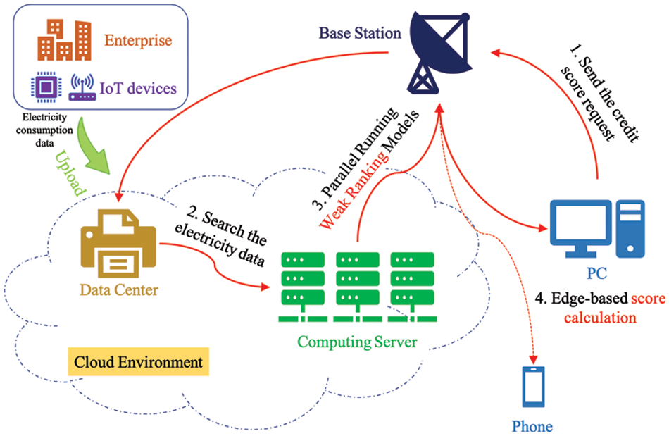
Figure 2: The structure of our edge computing framework

The core of this edge computing framework is to learn the proposed rankXGB model for credit scoring. To learn the rankXGB model, it should define the feature vector extracted from the raw electricity consumption data. After the training process of the rankXGB model, we deploy it in our edge computing environment. Due to a large number of weak ranking networks, it is not suitable to offload the network inference task in edge devices. Thus, we utilize the computing server in the cloud to realize the credit ranking. We then offload the ranking fusion in the edge terminal to reduce the burden of the computing server. The motivation is that the rankXGB model contains several independent weak ranking models, which can be run in parallel. Based on the observation, we utilize its distributed loosely coupling and high parallelism feature to integrate it into the edge computing framework. Since the size of the transmission data is rather small, the whole edge computing framework can be executed very efficiently.

In the following sections, we first introduce the representation of electricity consumption data including the feature vector and annotation in Section 3.1, then detail the training process of the rankXGB model in Section 3.2, and finally describe the inference process of the rankXGB model in Section 3.3.

3.1 The Representation of Electricity Consumption Data

Data representation is the basis of machine learning. As there are lots of different IoT devices in the power distribution system of the enterprise, a vast amount of electricity consumption data can be created. Since we cannot know a priori which type of data is related to credit scoring, we opt to include all the raw data except the identifier of the IoT device and its location code. Another thing is that the electricity consumption data is updated at any time. To improve the efficiency, we choose to use the latest data and make some statistics to compute the rate of change during a period.

To benefit the analysis of the scoring result, we recruit some energy experts to define a hierarchical structure according to the fields of electricity consumption data. As shown in Fig. 3, there are three levels in the hierarchical structure, and the indicators in the third level contain several fields.

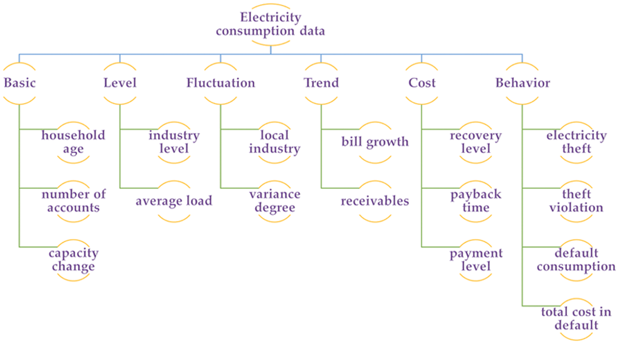
Figure 3: The hierarchical structure of enterprise consumption data

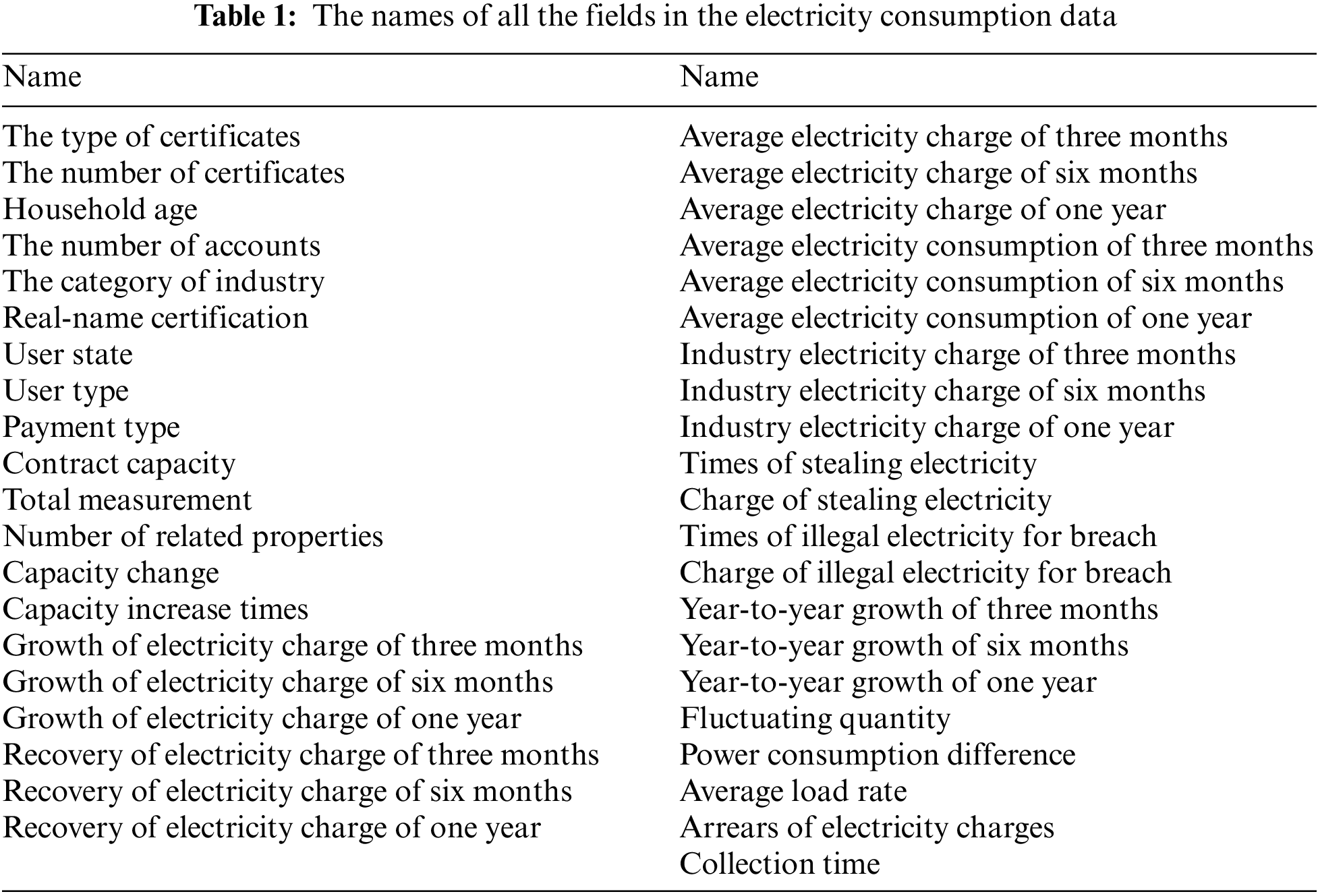
These fields might reflect the business state of the enterprises. For example, the household age and the number of accounts show the scale of the enterprise. The applied capacity change and the growth of electricity bills imply the potentiality of the enterprise. The credit analysis is also based on the operation and management level, which is related to the cumulative capacity increase and the average load ratio. For market competitiveness and cash flow, it is effective to check the industry level of electricity bills and fluctuation. The names of all the fields are shown in Table 1, and there are a total of 41 fields. Accordingly, we define a 41D feature vector to represent the electricity consumption data of the enterprise.

Based on the feature vector, we collect a large amount of electricity consumption data by the IoT device for many enterprises, which provides the training data as the basis of our rankXGB model. When collecting the training data, some fields might be missed due to storage problems. To fill the fields, we set them as the average of all the corresponding values. After the data collection, we recruit several financial analysts to annotate the data, which produces our training data set SI. As the rankXGB model relies on a pairwise relationship, each training data contains a pair of enterprises, which is defined as:

{(x1,x2),y}(1)

where the feature vectors x1 and x2 are the two consumption feature vectors of a pair of enterprises, and y∈[−1,0,+1] is the label to show the relative credit ranking. The annotation is simple, and we show two enterprises for all the experts at one time. If most of the experts think the first enterprise has a higher credit score than the second one, we set the label y as +1. Otherwise, we set the label y as −1. If the experts cannot determine which enterprise has a larger credit score, we set the label as 0 to avoid the inaccuracy annotation. After labeling all the pairwise relationships, the initial training dataset SI is generated. To guarantee the quality of the annotation, we also request that some financial institutions evaluate the relative credit relation from the business clues, such as the social, fiscal, and behavioral data. After comparing the annotation results, we only retain the annotation consistent from the electricity consumption and business perspectives. By analyzing the final annotation, we find that most enterprises are manufacturing enterprises. The reason is that there is a clear relationship between the manufacturing operation state and the electricity consumption data. For manufacturing enterprises, electricity consumption usually implies the timing of the production activities. With the increase in production time, the yield is likely to increase. Besides, the growth of the electric charge and the capacity increase times reflect the scale increase of the manufacturing enterprises. However, for other enterprises, such as services companies, the correlation between credit degree and electricity consumption is not high.

3.2 The Training of the RankXGB Model

Inspired by the pairwise method ranknet [50], we combine multilayer perceptron (MLP) and ranknet into a deep learning architecture. The multilayer perceptron is used to encode the 41D input feature vector for representation enhancement. To boost the performance, we add an XGBoost layer as the last layer of the architecture. We add such a layer since we use a lightweight MLP for feature encoding, which may not be sufficient to obtain a satisfactory result. There are also other boosting methods for prediction fusion, such as adaptive boosting (Adaboost) and GBDTs. Adaboost focuses on the weight of the training samples, while GBDTs optimize the performance of the classification by adding more trees. XGBoost also utilizes tree boosting to realize an effective ensemble learning system, but the main idea is to define a novel loss function and utilize its first and second derivatives for boosting. This improves the generalization ability significantly, and the loss function is easy to be integrated into the ranknet.

Another problem is that existing learn-to-rank methods all assume that the annotations are accurate. But in our application, the ranking markers given by users are not necessarily accurate, which will reduce the learned model effect. To address this issue, our method first uses sample selection to generate a more accurate training data set S and then uses the rankXGB model for training. Fig. 4 shows the two stages of our learning process: sample selection and model learning.

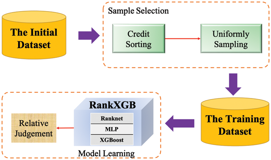
Figure 4: The learning process of the rankXGB model

Sample selection. The input is the initial training set SI after data collection and annotation, and the output is a subset S of the set SI by choosing some representative samples. Our motivation is that the set is not suitable for model training due to low-quality labeling. First, lots of the labels are 0, since the relative relationship is unclear. Second, we found the labels contain some contradictions. The unclear and inconsistent annotation fails to meet the requirements of the learning-to-rank algorithm. To solve it, we propose a ranking-based sample selection method.

Our idea is to sort all the samples into a sequence according to the biased order relationship. Then, the samples are selected uniformly from the sequence to generate the final training data set. As the successively selected samples are not adjacent in the initial sequence, the relative relation is reliable by increasing the sampling interval. The ranking-based sample selection method contains two steps: credit sorting and uniform sampling.

First, we sort the enterprises according to the relative credit relation. However, some elements are not comparable and inconsistency exists across all the relative credit labels. Thus, we combine a directed graph de-loop algorithm and a topological sort algorithm to sort the enterprises. This algorithm is based on a directed graph, which uses the enterprise as the graph node. To generate the edge of the graph, we search the set SI to obtain all the labels that are equal to +1 and generate an edge from the first enterprise to the second one. Since some labels are inconsistent, the graph contains some loops, as shown in Fig. 5a. Thus, we employ the directed graph de-loop algorithm to remove all the loops in the directed graph. To detect the loops of the graph, a depth-first searching algorithm is used to traverse the graph. If detecting a loop, we randomly select an edge in the loop and remove it from the graph. The process is repeated until no loop is found. Fig. 5b shows the directed graph after removing all the loops.

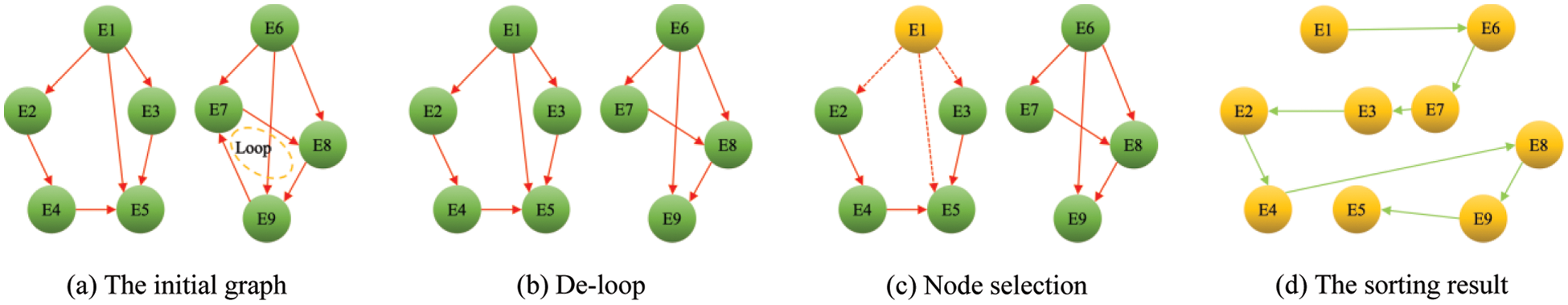
Figure 5: The process of credit sorting

After obtaining the directed acyclic graph, we use a topological sorting algorithm to generate a full-order list. The algorithm iteratively finds the nodes that have no incoming edges and add one of the nodes to a list. Then the node is removed from the graph. As shown in Fig. 5c, node ‘E1’ has no incoming edge and is selected as the first node. When removing the node ‘E1’, the edges that start from ‘E1’ are also removed (the red dot-dash lines). When the graph is empty, all the nodes form a full-order list, and the elements in the front of the list have larger credit scores. Fig. 5d shows the sorting result.

It is worth noting that the sorting list is not unique. Thus, given a pair of adjacent elements in the list, the relative information is not reliable. To improve the reliability, we select one enterprise from the sequence by uniform sampling to create the training data set. The sampling interval is indicated as b. As the list is generated according to the ascending order of the credit score, all the pairwise labels of the selected enterprise can be given. Accordingly, the final training dataset S is created for model training.

Model training. We then use the training dataset S to learn our rankXGB. The architecture of the rankXGB is shown in Fig. 6. The input layer receives two feature vectors of two enterprises as the input. The model contains two parts: feature encoding and relative credit prediction. The feature encoding part is designed by MLP, while the relative credit prediction part is created by an XGBoost layer.

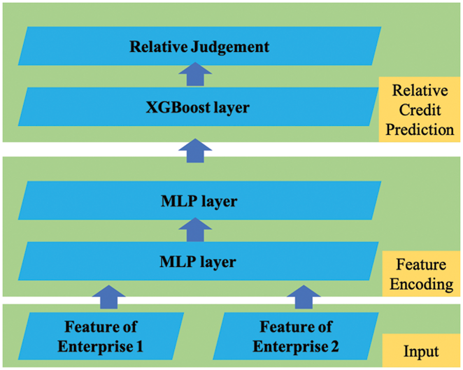
Figure 6: The architecture of the rankXGB model

The feature encoding part is used for feature learning. To reduce the latency of the edge computing framework, we use two hidden fully connected layers to generate a lightweight MLP network. The neurons of the fully connected layer are connected to all neurons of the previous layer. The sizes of the two hidden layers are t and s, respectively. To avoid overfitting, one dropout layer is inserted between the two MLP layers. For the activation function, we choose the rectified linear unit function. Obviously, we can add more hidden layers in our feature encoding part. However, the increase in the number of layers can increase the inference timing of the network. As shown in Fig. 6, all the weak ranking models share the same MLP weights, which reduces the model complexity and prevents overfitting effectively.

The relative credit prediction part judges which input enterprise has a higher credit score given the feature encoding result. We use the XGBoost layer to improve the robustness of the ranking models. Instead of using decision trees, we choose to use neural networks to realize the model fusion. The XGBoost layer realizes an ensemble of K weak ranking models by fusing the predictions of all the weak models.

y^=φ(x1,x2)=∑k=1Kfk(x1,x2)(2)

where y^ is the final prediction, fk is the prediction score of the k-th weak ranking model, x1 and x2 are the two consumption feature vectors of two enterprises. To prevent overfitting, we add a regularization function to control the complexity of the weak ranking model f as follows.

Ω(f)=12λ‖w‖2(3)

where Ω(f) is the measurement of the complexity of the learned model f, which is the sum of the squares of the weight w including the weights of the MLP layers. λ is the weighting factor to measure the importance of regularization. Following the design of the neural network boost algorithm [15], we learn the k-th weak ranking model to fit the residual of the previous ranking model.

Rk=y−fk−1(x1,x2)(4)

where y is the expected prediction score, Rk is the residual of the k-th ranking model. Accordingly, the first model fits the expected prediction score y, and the second model fits the score residual of the first model. Thus, the final score residual can be reduced by adding more weak ranking models. By fitting all the score residuals successively, the final prediction is the sum of all the prediction scores of K weak models.

Each ranking model judges which enterprise has a higher credit score, which is a binary classification task. Thus, we use the entropy loss as our objective function to show the ranking constraints, and the entropy loss of the k-th model is defined as:

Lk=12(1−Rk)σfk(x1,x2)+log⁡(1+e−σfk(x1,x2))(5)

where σ is a constant hyper parameter.

Accordingly, the objective function is defined by adding the loss and the regularization function.

Obj=∑k=1KLk+Ω(f)(6)

Based on the above objective function, we use the gradient descent method to optimize the weight of the ranking model. These weak models are learned successively, and every model is learned to fit the last residual. This makes the sum of all the weak models fit the expected prediction.

3.3 The Inference of the RankXGB Model

After getting the learned rankXGB model, we deploy the model in our edge computing framework. To reduce the burden of the cloud server, we offload the prediction fusion task in the edge terminal, and the deployment is illustrated in Fig. 7. As shown in the figure, the weak ranking models are deployed in the cloud server to compare the credit score of a test enterprise with every training enterprise. The ranking fusion is executed in the edge terminal after receiving the weak ranking results from the cloud server. An absolute credit score is finally generated by the score normalization in the terminal.

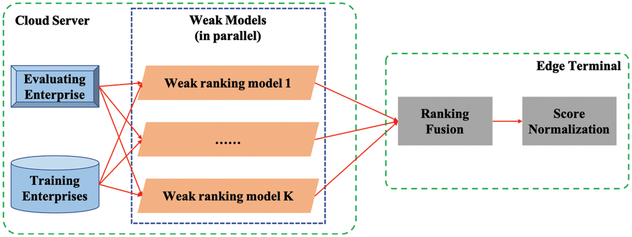
Figure 7: The deployment of the rankXGB model in the edge computing framework

To ease the credit analysis, the goal of our edge computing framework is to generate the absolute credit score of an enterprise, which cannot be generated by our learned rankXGB model directly. To solve it, we save all the enterprises in the initial training set SI as the benchmark enterprises in the cloud server. If the users expect to know the credit score of an enterprise, we use our ranking model to compare its credit score with all the benchmark enterprises. The relative judgment task is completed by utilizing the computing resource of the cloud server and the edge terminal. The cloud server generates multiple relative judgments by the set of weak ranking models in our rankXGB model. Since the forward propagation of the weak models is independent, we can run the weak ranking models in parallel or even at different servers. All the prediction scores are sent to the edge terminal for ranking fusion, and the final ranking results are obtained by accumulating the prediction scores with a simple sum operation. It is also feasible to offload the ranking fusion step in the cloud. But in practice, the weak ranking models might be executed in different servers. To avoid redundant information transmission, we choose to execute this task in the edge terminal due to its low computational complexity.

By the ranking fusion, we can know the relative judgments between the test enterprises and every benchmark enterprise. To generate the absolute credit score of the given enterprise, we use a mapping function as a score normalization process. The mapping function computes the percentile position of the test enterprise in the set SI. The percentile position is then used as the final absolute credit score of the enterprise. For example, if the credit score of the enterprise is larger than 52.2% of the samples in the set SI, its absolute credit score is set as 52.2.

4  Experiment

In this section, we evaluate our proposed enterprise credit score method based on deep learning in the edge computing framework.

4.1 Experimental Setup

To evaluate the effectiveness of our method, we collect the electricity consumption data of some enterprises, which consists of 10,593 training samples and 1,637 test samples. When learning the rankXGB model, we set the initial learning rate, the number of training iterations, and the batch size as 1×10−3, 100, and 64, respectively. During the training process, we use the linear decay strategy to adjust the learning rate. All the experiments are performed with an NVIDIA GTX3090 GPU, and we use Pytorch to implement the learning of our model.

4.2 Experimental Criteria

To assess the effectiveness of the model, Normalized Discounted Cumulative Gain (NDCG) is used as the evaluation criterion. NDCG is computed by:

NDCG=∑i=1p2reli−1log2⁡(i+1)∑i=1|REL|relilog2⁡(i+1)(7)

where reli is the graded relevance of the result at the i-th position, and REL is the list of relevant elements. NDCG is widely used to evaluate learning-to-rank algorithms.

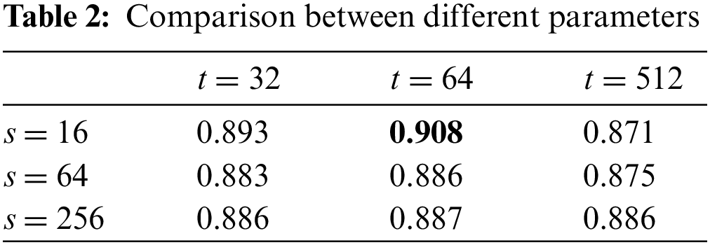
4.3 The Comparison between Different MLP Parameters

As described in Section 3.2, the feature encoding part is realized by a lightweight MLP network, which has two hidden layers. The sizes of the layers are t and s, respectively. To search the optimal values of the parameters t and s, this experiment executes our approach with different values. The candidate values of the parameter t include 32, 64, and 512, while the candidate values of the parameter s are 16, 64, and 256. Based on the different values, the rankXGB model is learned by using only one network. The final performance is measured by NDCG. The results are shown in Table 2. From the comparison, we can see that the performances under different parameter settings are almost the same. The result shows that the model achieves the best performance when t = 64 and s = 16. Thus, we choose to use t = 64 and s = 16 for the following experiments.

4.4 The Comparison between Different Sampling Intervals

To improve the robustness of our rankXGB model, we execute the sample selection operation to remove the unreliable annotation. The last step is uniform sampling, which selects a sample from a list of every b enterprises. To evaluate the influence of the sampling intervals, we execute this evaluation experiment by using different values, which range from 20 to 150. We utilize these 14 candidate values as the sampling intervals to generate different training datasets. Accordingly, we learn different rankXGB models without the XGBoost layer and compute the performance by NDCG.

As shown in Fig. 8, this parameter has a significant impact on the performance of the learned model. If the parameter is small, the performance is low, since unreliable annotation still exists. With the increase of the parameter, the performance is first improved to a peak value and then dropped gradually. This reason is that the oversized sampling interval might discard many samples. Thus, the limited training dataset cannot meet the requirement of deep learning, which reduces the performance of the learned model. From the result, the optimal value is 100, which achieves the best accuracy.

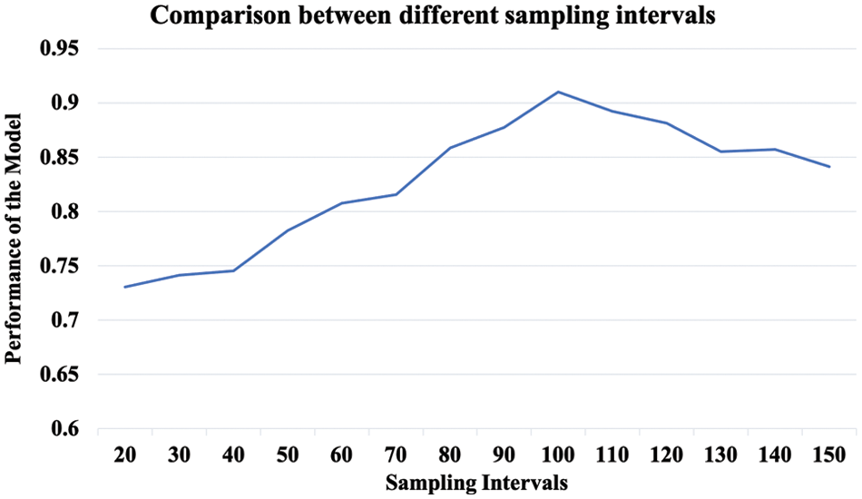
Figure 8: The comparison between different sampling intervals

4.5 The Parameter Analysis of the XGBoost Layer

There are two important parameters in the XGBoost layer. The first one is the number of weak ranking models K, while the second one is the weight factor λ for regularization. To analyze the effect of these two parameters, we design two parameter experiments by setting different values for the parameters K and λ. The experimental results are shown in Fig. 9. In Fig. 9a, we illustrate the performance of the learned model with the increasing number of weak ranking models. From the figure, we can see that 4 networks reach the highest NDCG, but more networks make the performance degrade slightly. When the number of neural networks is larger than 9, the performance is lower than a single neural network. The reason is that more parameters lead to overfitting, which decreases generalization performance and promotion of capacity. In Fig. 9b, we describe the relationship between the performance of the learned model and the weight factor λ. From the figure, we can see that it has a great influence on the final performance. When λ is equal to 0.3, it achieves the best effect. The reason is that when λ is large, the model complexity is suffered from severe constraints, which cannot capture the relationship between the credit degree and the electricity consumption accurately.

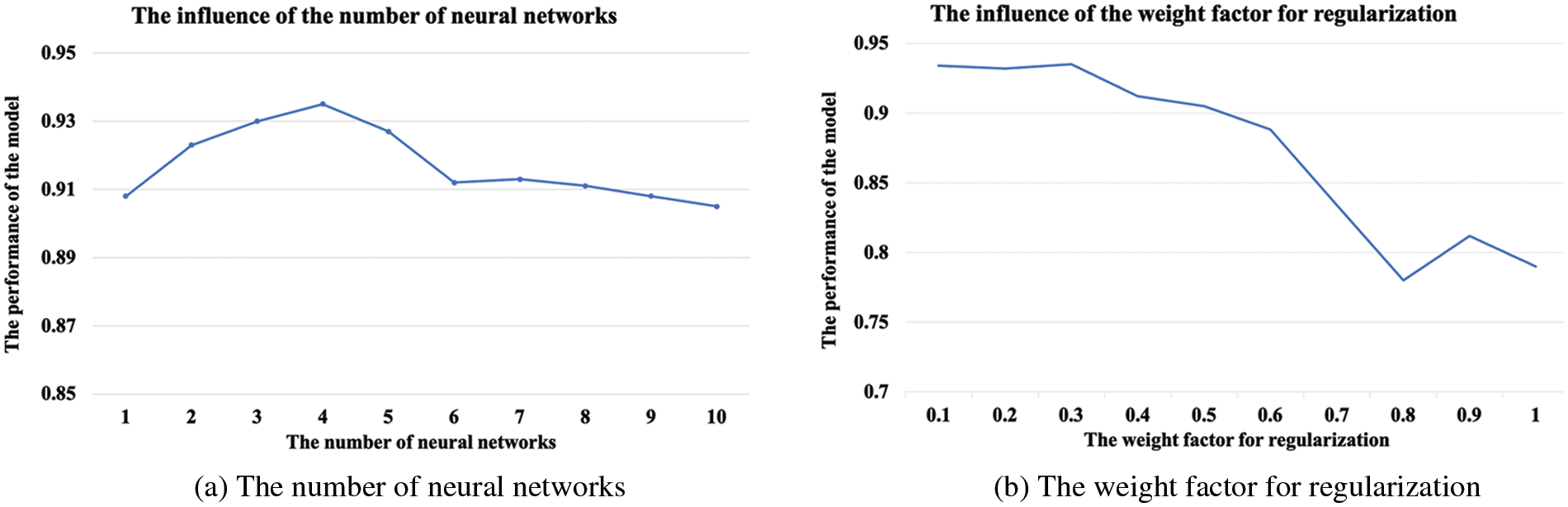
Figure 9: The parameter analysis of the XGBoost layer

4.6 The Comparison with Alternative Methods

In this section, we perform the comparison experiment with some alternative methods. The first method is deep regression (DR). To realize it, we first generate the training enterprises by the same method as ours. Then, the pairwise ranking annotation is used to compute the absolute credit scores of the training enterprises by the score normalization as described in Section 3.3. For the network architecture, we follow the same design of our network but replace the last XGBoost layer with a regression layer. We also remove the XGBoost layer to train a single deep ranknet for credit scoring. To show the technical choice of the MLP network, we also replace our MLP structure with the other deep networks, including 1D convolutional neural network (1D-CNN) [68] and transformer [69].

Existing credit scoring methods usually treat the credit scoring method as a classification method. To compare with these methods, we turn the ranking problem into a classification problem. The training dataset is created in the same way, and the credit rating is obtained by splitting the whole set into 10 credit levels according to the descending order of enterprise credit. The granularity of the credit levels is very important, and we also try 5 and 20 levels. When splitting the set into 5 levels, the classification accuracy is very high. However, the granularity is too coarse to distinguish the relative credit relation between many pairs of enterprises. When the number of levels is 20, the classification accuracy degrades, which leads to a low NDCG. Thus, we set the number of credit levels as 10. Based on such a dataset, we can utilize existing credit scoring methods for performance comparison. It is worth noting that existing credit scoring methods all use business data for credit analysis. Though electricity consumption data shows different cues, the data process is the same, which maps a given feature vector into a category label. We choose the methods described in the recent two credit score benchmarks [3,70]. Among these methods, we select the following classifiers: random forest (RF), logistic regression (LR), SVM, XGboost, naive bayes (NB), and MLP.

Fig. 10a shows the comparison result. From the comparison, we found that the performance of our method is higher than that of the other methods. It is clear that all of the classification methods perform much worse than the ranking and regression method. The reason is that the classification model does not consider the relative ranking between the credit level. As a result, the loss of the ranking information leads to a lower NDCG. Compared with the deep regression method, the ranking model usually performs better if the learned deep network fits the task. Due to the complex relationship between credit score and electricity consumption, the deep regression method requires a deeper network to capture the relationship accurately. In contrast, the ranking model treats the task as a binary classification problem, and our lightweight network is able to achieve a satisfactory effect. However, the network architecture should match the characteristics of data representation. As the dimension of the consumption feature vector has no relation to its position, the 1D-CNN network does not perform well due to the limited connection between the network layers.

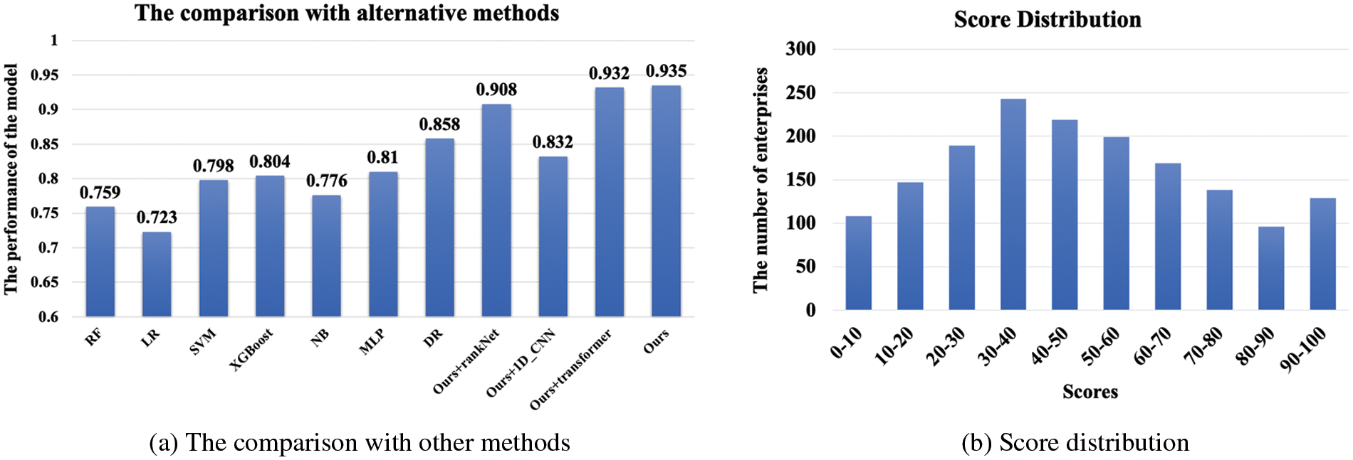
Figure 10: The comparison with other methods and score distribution

We also show our score normalization result of some test enterprises in Fig. 10b, and the whole distribution is near the normal distribution. This score distribution matches the general cognition of human beings, as most enterprises have a moderate credit degree.

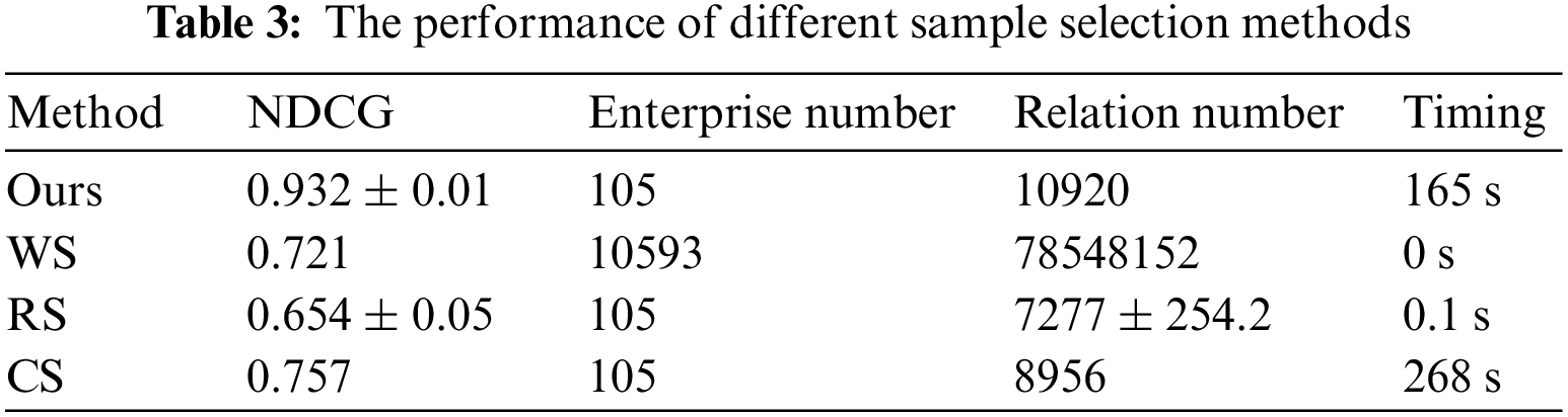
4.7 The Evaluation of Sample Selection

We compare our sample selection method with the following baseline methods: without selection (WS), random selection (RS), and clustering-based selection (CS). All the sample selection methods select the same number of samples. To realize the clustering-based selection, we use the mean shift algorithm to classify all the enterprises in the initial dataset SI into several clusters. We set the bandwidth as a quarter of the maximum pairwise distance between all the enterprises. After the clustering, we choose the enterprise as the training sample that has the nearest distance to the corresponding cluster center. After the selection, we remove these selected samples and execute the clustering process on the remained samples. The selection process is repeated until enough samples are selected. Based on different selected samples, we learn different rankXGB models and compare their performances. Since the result of RS and ours are affected by the random process, we run each of the two methods 10 times and compute the mean and the standard deviation. The result is shown in Table 3. From the table, we can see our method outperforms the other methods from the NDCG metric impressively. This proves that our method can improve the quality of the training dataset effectively. Compared with the RS method, our method produces a more stable result due to the lower standard deviation. Table 3 also shows the other indicators, including the enterprise number, the relation number (the relative label is not 0), and the sampling timing. All the sampling methods select 105 enterprises from the training samples. Since the other two sampling methods do not sort all the selected enterprises, the relation numbers of these two methods are smaller than ours. For efficiency, the timing of random selection is the fastest, while the clustering-based selection method spends the most time due to the complexity of the mean-shift clustering method.

4.8 Complexity Analysis

The proposed method runs in the edge computing environment with mobile or terminal edge devices. According to our measurements, when uploading the consumption data from the data center to the computing server, the electricity consumption data is compressed and transmitted in 30 milliseconds under a fourth-generation cellular network. The inference of the cloud-based weak credit ranking process spends about 5 milliseconds. Afterward, it also costs 10 milliseconds to transfer the sorting results to the edge devices and the edge-based enterprise credit score calculation process takes about 10 milliseconds on a mobile device. The mobile phone is adopted as Huawei Pro30 with Kylin 990 chips. We also test it on a PC device with Intel (Registered trademark) Core (Trade mark) i5-2400 3.10 GHz, which takes about 2 milliseconds. The above measurements show that our method can support real-time credit scoring applications.

5  Conclusions

In this paper, we propose a rankXGB-based enterprise credit scoring method in an edge computing framework. The enterprise credit is obtained by analyzing the electricity consumption data captured by various IoT devices. This method designs a two-stage deep learning architecture, including two stages: the cloud-based enterprise weak credit ranking and the edge-based enterprise credit score calculation. In the first stage, we send the electricity consumption data of the enterprise to the cloud and execute multiple weak ranking networks in parallel in the servers to calculate the credit ranking relationship between the test enterprise and the benchmark enterprises. In the second stage, we execute the post-processing of the deep ranking network in the edge terminal, which includes the ranking fusion and the score normalization process. The final experimental results prove that this method can achieve accurate enterprise credit evaluation as a real-time application.

Limitation and future work. The robustness and effectiveness of our method have been demonstrated by extensive experiments. However, the amount of the relative credit annotation is much larger than that of the regression setting. Therefore, our method can combine some active learning methods to reduce the cost of the annotation further. Another limitation is that the score normalization process relies on the training dataset. If one enterprise has a higher credit degree than all the training samples, we cannot obtain its credit score precisely. Thus, a dynamic updating mechanism is required to update the training dataset, when the training dataset is insufficient to show the complete credit range of the enterprises. Another direction is to combine the social, fiscal, and behavioral data into our model for a more effective credit evaluation framework.

Acknowledgement: This research was funded by National Natural Science Foundation of China (61906036), Science and Technology Project of State Grid Jiangsu Power Supply Company (No. J2021034).

Funding Statement: This research was funded by National Natural Science Foundation of China (61906036), Science and Technology Project of State Grid Jiangsu Power Supply Company (No. J2021034).

Conflicts of Interest: The authors declare that they have no conflicts of interest to report regarding the present study.

References

    1. Z. Wang, L. Jia, M. Li, S. Yang, Y. Wang et al., “Edge computing and blockchain in enterprise performance and venture capital management,” Computational Intelligence and Neuroscience, vol. 2022, no. 1, pp. 2914936–2914939, 2022. [Google Scholar]

    2. X. Dastile, T. Celik and M. Potsane, “Statistical and machine learning models in credit scoring: A systematic literature survey,” Applied Soft Computing, vol. 91, no. 2, pp. 106263, 2020. [Google Scholar]

    3. V. Moscato, A. Picariello and G. Sperlí, “A benchmark of machine learning approaches for credit score prediction,” Expert Systems with Applications, vol. 165, no. 9, pp. 113986, 2021. [Google Scholar]

    4. J. Yuan, C. Zhao, S. Yu and Z. Hu, “Electricity consumption and economic growth in China: Cointegration and co-feature analysis,” Energy Economics, vol. 29, no. 6, pp. 1179–1191, 2007. [Google Scholar]

    5. K. Abbasi, J. Abbas and M. Tufail, “Revisiting electricity consumption, price, and real GDP: A modified sectoral level analysis from Pakistan,” Energy Policy, vol. 149, pp. 112087, 2021. [Google Scholar]

    6. C. Beckel, L. Sadamori and S. Santini, “Automatic socio-economic classification of households using electricity consumption data,” in Proc. 4th Int. Conf. on Future Energy Systems (e-Energy '13), Berkeley, California, USA, pp. 75–86, 2013. [Google Scholar]

    7. C. Luo, D. Wu and D. Wu, “A deep learning approach for credit scoring using credit default swaps,” Engineering Applications of Artificial Intelligence, vol. 65, no. 2, pp. 465–470, 2017. [Google Scholar]

    8. C. Wang, D. Han, Q. Liu and S. Luo, “A deep learning approach for credit scoring of peer-to-peer lending using attention mechanism LSTM,” IEEE Access, vol. 7, pp. 2161–2168, 2018. [Google Scholar]

    9. Z. Zhang, K. Niu and Y. Liu, “A deep learning based online credit scoring model for P2P lending,” IEEE Access, vol. 8, pp. 177307–177317, 2020. [Google Scholar]

  10. M. Song, X. Han, X. Liu and Q. Li, “Visibility estimation via deep label distribution learning in cloud environment,” Journal of Cloud Computing, vol. 10, no. 1, pp. 1–14, 2021. [Google Scholar]

  11. X. Burgos-Artizzu, P. Perona and P. Dollár, “Robust face landmark estimation under occlusion,” in Proc. 2013 IEEE Int. Conf. on Computer Vision, Sydney, Australia, pp. 1513–1520, 2013. [Google Scholar]

  12. L. Qi, W. Lin, X. Zhang, W. Dou, X. Xu et al., “A correlation graph-based approach for personalized and compatible web APIs recommendation in mobile APP development,” IEEE Transactions on Knowledge and Data Engineering, pp. 1–14, 2022. https://doi.org/10.1109/TKDE.2022.3168611. [Google Scholar]

  13. A. Javadpour, K. Saedifar, G. Wang, K. Li and F. Saghafi, “Improving the efficiency of customer's credit rating with machine learning in big data cloud computing,” Wireless Personal Communications, vol. 121, no. 4, pp. 2699–2718, 2021. [Google Scholar]

  14. S. Thongsuwan, S. Jaiyen, A. Padcharoen and P. Agarwalc, “ConvXGB: A new deep learning model for classification problems based on CNN and XGBoost,” Nuclear Engineering and Technology, vol. 53, no. 2, pp. 522–531, 2021. [Google Scholar]

  15. J. Dong, Y. Chen, B. Yao, X. Zhang and N. Zeng, “A neural network boosting regression model based on XGBoost,” Applied Soft Computing, vol. 125, no. 1, pp. 109067, 2022. [Google Scholar]

  16. Z. Cao, T. Qin, T. Liu, M. Tsai and H. Li, “Learning to rank: From pairwise approach to listwise approach,” in Proc. 24th Int. Conf. on Machine Learning, Corvalis Oregon, USA, pp. 129–136, 2007. [Google Scholar]

  17. L. Hodgkinson and E. Walker, “An expert system for credit evaluation and explanation,” Journal of Computing Sciences in Colleges, vol. 19, no. 1, pp. 62–72, 2003. [Google Scholar]

  18. V. Cateté and T. Barnes, “Application of the delphi method in computer science principles rubric creation,” in Proc. 2017 ACM Conf. on Innovation and Technology in Computer Science Education (ITiCSE '17), Bologna, Italy, pp. 164–169, 2017. [Google Scholar]

  19. B. Feng and W. Xue, “Contrastive pre-training for imbalanced corporate credit ratings,” in Proc. 14th Int. Conf. on Machine Learning and Computing (ICMLC), Guangzhou, China, pp. 293–297, 2022. [Google Scholar]

  20. X. Yang and S. Jiang, “The construction of big data credit evaluation system in the management of indemnificatory housing access,” in Proc. 3rd Int. Work. on Education, Big Data and Information Technology (EBDIT 2019), Guilin, China, pp. 98–101, 2019. [Google Scholar]

  21. K. Thaker, P. Carvalho and K. Koedinger, “Comprehension factor analysis: Modeling student's reading behaviour: Accounting for reading practice in predicting students' learning in MOOCs,” in Proc. 9th Int. Conf. on Learning Analytics & Knowledge (LAK19), Tempe, Arizona, USA, pp. 111–115, 2019. [Google Scholar]

  22. Y. Fang, Y. Zhang and C. Huang, “Credit card fraud detection based on machine learning,” Computers, Materials & Continua, vol. 61, no. 1, pp. 185–195, 2019. [Google Scholar]

  23. W. Liu, H. Fan and M. Xia, “Credit scoring based on tree-enhanced gradient boosting decision trees,” Expert Systems with Applications, vol. 189, no. 1, pp. 116034, 2022. [Google Scholar]

  24. W. Liu, H. Fan and M. Xia, “Multi-grained and multi-layered gradient boosting decision tree for credit scoring,” Applied Intelligence, vol. 52, no. 5, pp. 5325–5341, 2022. [Google Scholar]

  25. S. Li, W. Shiue and M. Huang, “The evaluation of consumer loans using support vector machines,” Expert Systems with Applications, vol. 30, no. 4, pp. 772–782, 2006. [Google Scholar]

  26. D. West, “Neural network credit scoring models,” Computers & Operations Research, vol. 27, no. 11–12, pp. 1131–1152, 2000. [Google Scholar]

  27. J. Zhang and Q. Xu, “Attention-aware heterogeneous graph neural network,” Big Data Mining and Analytics, vol. 4, no. 4, pp. 233–241, 2021. [Google Scholar]

  28. C. Chen, J. Jiang, Y. Zhou, N. Lv, X. Liang et al., “An edge intelligence empowered flooding process prediction using Internet of things in smart city,” Journal of Parallel and Distributed Computing, vol. 165, pp. 66–78, 2022. [Google Scholar]

  29. M. Song, Y. Liu and X. Liu, “Semi-supervised 3D shape recognition via multimodal deep co-training,” Computer Graphics Forum, vol. 39, no. 7, pp. 279–289, 2020. [Google Scholar]

  30. Y. Wu, H. Guo, C. Chakraborty, M. Khosravi, S. Berretti et al., “Edge computing driven low-light image dynamic enhancement for object detection,” IEEE Transactions on Network Science and Engineering, pp. 1–14, 2022. https//doi.org/10.1109/TNSE.2022.3151502. [Google Scholar]

  31. Y. Wu, Y. Ma and S. Wan, “Multi-scale relation reasoning for multi-modal visual question answering,” Signal Processing: Image Communication, vol. 96, pp. 116319, 2021. [Google Scholar]

  32. W. Liu, G. Wu, F. Ren and X. Kang, “DFF-ResNet: An insect pest recognition model based on residual networks,” Big Data Mining and Analytics, vol. 3, no. 4, pp. 300–310, 2020. [Google Scholar]

  33. W. Cai, Y. Wang, J. Ma and Q. Jin, “Can: Effective cross features by global attention mechanism and neural network for ad click prediction,” Tsinghua Science and Technology, vol. 27, no. 1, pp. 186–195, 2022. [Google Scholar]

  34. X. Xu, T. Gao, Y. Wang and X. Xuan, “Event temporal relation extraction with attention mechanism and graph neural network,” Tsinghua Science and Technology, vol. 27, no. 1, pp. 79–90, 2022. [Google Scholar]

  35. Y. Yang, N. Zhu, Y. Wu, J. Cao, D. Zhan et al., “A semi-supervised attention model for identifying authentic sneakers,” Big Data Mining and Analytics, vol. 3, no. 1, pp. 29–40, 2020. [Google Scholar]

  36. F. Liu, Z. Zhang and R. Zhou, “Automatic modulation recognition based on CNN and GRU,” Tsinghua Science and Technology, vol. 27, no. 2, pp. 422–431, 2022. [Google Scholar]

  37. G. Zhai, Y. Yang, H. Wang and S. Du, “Multi-attention fusion modeling for sentiment analysis of educational big data,” Big Data Mining and Analytics, vol. 3, no. 4, pp. 311–319, 2020. [Google Scholar]

  38. W. Liang, Y. Hu, X. Zhou, Y. Pan and I. Kevin, “Variational few-shot learning for microservice-oriented intrusion detection in distributed industrial IoT,” IEEE Transactions on Industrial Informatics, vol. 18, no. 8, pp. 5087–5095, 2021. [Google Scholar]

  39. X. Zhou, W. Liang, W. Li, K. Yan, S. Shimizu et al., “Hierarchical adversarial attacks against graph neural network based IoT network intrusion detection system,” IEEE Internet of Things Journal, vol. 9, no. 12, pp. 9310–9319, 2022. [Google Scholar]

  40. L. Qi, Y. Yang, X. Zhou, W. Rafique and J. Ma, “Fast anomaly identification based on multi-aspect data streams for intelligent intrusion detection toward secure industry 4.0,” IEEE Transactions on Industrial Informatics, vol. 18, no. 9, pp. pp 6503–6511, 2022. [Google Scholar]

  41. Y. Liu, D. Li, S. Wan, F. Wang, W. Dou et al., “A long short-term memory-based model for greenhouse climate prediction,” International Journal of Intelligent Systems, vol. 37, no. 1, pp. 135–151, 2022. [Google Scholar]

  42. J. Dong, W. Wu, Y. Gao, X. Wang and P. Si, “Deep reinforcement learning based worker selection for distributed machine learning enhanced edge intelligence in internet of vehicles,” Intelligent and Converged Networks, vol. 1, no. 3, pp. 234–242, 2020. [Google Scholar]

  43. Y. Liu, Z. Song, X. Xu, W. Rafique, X. Zhang et al., “Bidirectional GRU networks-based next POI category prediction for healthcare,” International Journal of Intelligent Systems, vol. 37, no. 7, pp. 4020–4040, 2021. [Google Scholar]

  44. X. Zhao, Z. Wang, L. Gao, Y. Li and S. Wang, “Incremental face clustering with optimal summary learning via graph convolutional network,” Tsinghua Science and Technology, vol. 26, no. 4, pp. 536–547, 2021. [Google Scholar]

  45. D. Babaev, M. Savchenko, A. Tuzhilin and D. Umerenkov, “Et-rnn: Applying deep learning to credit loan applications,” in Proc. 25th ACM SIGKDD Int. Conf. on Knowledge Discovery & Data Mining, Anchorage, AK USA, pp. 2183–2190, 2019. [Google Scholar]

  46. C. Wu, S. Huang, C. Chiou and Y. Wang, “A predictive intelligence system of credit scoring based on deep multiple kernel learning,” Applied Soft Computing, vol. 111, no. 1, pp. 107668, 2021. [Google Scholar]

  47. D. Cossock and T. Zhang, “Subset ranking using regression,” in Proc. Int. Conf. on Computational Learning Theory, Pittsburgh, PA, USA, pp. 605–619, 2006. [Google Scholar]

  48. P. Li, Q. Wu and C. Burges, “Mcrank: Learning to rank using multiple classification and gradient boosting,” in Proc. 20th Int. Conf. on Neural Information Processing Systems, Vancouver British Columbia, Canada, pp. 897–904, 2007. [Google Scholar]

  49. S. Dutta, X. Liu, A. Biswas and H. Shen, “Pointwise information guided visual analysis of time-varying multi-fields,” in SIGGRAPH Asia 2017 Symp. on Visualization (SA '17), Bangkok, Thailand, pp. 1–8, 2017. [Google Scholar]

  50. C. Burges, T. Shaked, E. Renshaw and A. Lazier, “Learning to rank using gradient descent,” in Proc. 22nd Int. Conf. on Machine learning, Bonn, Germany, pp. 89–96, 2005. [Google Scholar]

  51. L. Rigutini, T. Papini and M. Maggini, “Sortnet: Learning to rank by a neural-based sorting algorithm,” in Proc. SIGIR 2008 Work. on Learning to Rank for Information Retrieval (LR4IR), Singapore, Singapore, pp. 76–79, 2008. [Google Scholar]

  52. C. Burges, R. Ragno and Q. Le, “Learning to rank with non-smooth cost functions,” in Proc. 19th Int. Conf. on Neural Information Processing Systems, Vancouver British Columbia, Canada, pp. 193–200, 2006. [Google Scholar]

  53. R. Rahimi, A. Montazeralghaem and J. Allan, “Listwise neural ranking models,” in Proc. 2019 ACM SIGIR Int. Conf. on Theory of Information Retrieval (ICTIR '19), Santa Clara CA, USA, pp. 101–104, 2019. [Google Scholar]

  54. L. Qi, C. Hu, X. Zhang, M. Khosravi, S. Sharma et al., “Privacy-aware data fusion and prediction with spatial-temporal context for smart city industrial environment,” IEEE Transactions on Industrial Informatics, vol. 17, no. 6, pp. 4159–4167, 2021. [Google Scholar]

  55. B. Varghese, N. Wang and S. Barbhuiya, “Challenges and opportunities in edge computing,” in Proc. of 2016 IEEE Int. Conf. on Smart Cloud (SmartCloud), New York, USA, pp. 20–26, 2016. [Google Scholar]

  56. X. Zhou, X. Yang, J. Ma and I. Kevin, “Energy efficient smart routing based on link correlation mining for wire-less edge computing in IoT,” IEEE Internet of Things Journal, vol. 9, no. 16, pp. 14988–14997, 2021. [Google Scholar]

  57. X. Zhou, X. Xu, W. Liang, Z. Zeng and Z. Yan, “Deep-learning-enhanced multitarget detection for end-edge–cloud surveillance in smart iot,” IEEE Internet of Things Journal, vol. 8, no. 16, pp. 12588–12596, 2021. [Google Scholar]

  58. X. Xu, Z. Fang, J. Zhang, Q. He, D. Yu et al., “Edge content caching with deep spatiotemporal residual network for IoV in smart city,” ACM Transactions on Sensor Networks, vol. 17, no. 3, pp. 1–33, 2021. [Google Scholar]

  59. C. Chen, Y. Zhang, Z. Wang, S. Wan and Q. Pei, “Distributed computation offloading method based on deep reinforcement learning in ICV,” Applied Soft Computing, vol. 103, no. JUL, pp. 107108, 2021. [Google Scholar]

  60. X. Zhou, W. Liang, K. Yan, W. Li, I. Kevin et al., “Edge enabled two-stage scheduling based on deep reinforcement learning for internet of everything,” IEEE Internet of Things Journal, pp. 1–9, 2022. https://doi.org/10.1109/JIOT.2022.3179231. [Google Scholar]

  61. S. Nath and J. Wu, “Deep reinforcement learning for dynamic computation offloading and resource allocation in cache-assisted mobile edge computing systems,” Intelligent and Converged Networks, vol. 1, no. 2, pp. 181–198, 2020. [Google Scholar]

  62. H. Dai, Y. Xu, G. Chen, W. Dou, C. Tian et al., “ROSE: Robustly safe charging for wireless power transfer,” IEEE Transactions on Mobile Computing, vol. 21, no. 6, pp. 2180–2197, 2022. [Google Scholar]

  63. H. Dai, X. Wang, X. Lin, R. Gu, S. Shi et al., “Placing wireless chargers with limited mobility,” IEEE Transactions on Mobile Computing, pp. 1–15, 2021. https://doi.org/10.1109/TMC.2021.3136967. [Google Scholar]

  64. R. Gu, K. Zhang, Z. Xu, Y. Che and B. Fan, “Fluid: Dataset abstraction and elastic acceleration for cloud-native deep learning training jobs,” in Proc. 38th IEEE Int. Conf. on Data Engineering, Kuala Lumpur, Malaysia, Virtual Event, pp. 2183–2196, 2022. [Google Scholar]

  65. R. Gu, Y. Chen, S. Liu, H. Dai, G. Chen et al., “Liquid: Intelligent resource estimation and network-efficient scheduling for deep learning jobs on distributed GPU clusters,” IEEE Transactions on Parallel and Distributed Systems, vol. 33, no. 11, pp. 2808–2820, 2021. [Google Scholar]

  66. X. Zhou, Y. Hu, J. Wu, W. Liang, J. Ma et al., “Distribution bias aware collaborative generative adversarial network for imbalanced deep learning in industrial iot,” IEEE Transactions on Industrial Informatics, pp. 1–11, 2022. https://doi.org/10.1109/TII.2022.3170149. [Google Scholar]

  67. S. Liu, J. Yu, X. Deng and S. Wan, “FedCPF: An efficient-communication federated learning approach for vehicular edge computing in 6G communication networks,” IEEE Transactions on Intelligent Transportation Systems, vol. 23, no. 2, pp. 1616–1629, 2022. [Google Scholar]

  68. M. Alvarado-Gonzalez, G. Fuentes-Pineda and J. Cervantes-Ojeda, “A few filters are enough: Convolutional neural network for P300 detection,” Neurocomputing, vol. 425, no. 2, pp. 37–52, 2021. [Google Scholar]

  69. A. Vaswani, N. Shazeer, N. Parmar, J. Uszkoreit, L. Jones et al., “Attention is all you need,” in Proc. 31st Int. Conf. on Neural Information Processing Systems, Long Beach CA, pp. 6000–6010, 2017. [Google Scholar]

  70. D. Tripathi, D. Edla, A. Bablani, A. Shukla and B. Reddy, “Experimental analysis of machine learning methods for credit score classification,” Progress in Artificial Intelligence, vol. 10, no. 3, pp. 217–243, 2021. [Google Scholar]