A Levenberg–Marquardt Based Neural Network for Short-Term Load Forecasting

1  Introduction

Electric power load forecasting is essential for the planning and decision-making of power system management. Electric load generation, transmission, and distribution utilities heavily depend on load forecast. Therefore, these utilities need accurate methods to forecast electrical load to use their infrastructure effectively, safely, and economically [1,2]. Typically, load forecasting is categorized into four categories, i.e., very short-term (VSTLF), short-term (STLF), medium-term (MTLF), and long-term (LTLF) load forecasting. These are hourly, daily, weekly, and yearly forecasting [3]. Among all these, STLF is the most significant and challenging owing to its direct economic consequences. As there is no method of storing electrical energy and generating it instantly, the amount of electricity generated should be balanced with the amount used by the consumer. The producers’ economy could face difficulties if anticipated energy production is not balanced. Energy companies lose a lot of money due to imbalance load forecasting, e.g., a 1% increase in forecasted load due to miscalculation is nearly equivalent to a $10 million increase in the operational cost of the power plants [4]. Therefore, there is a need that power producers must generate balanced electricity in production, distribution, transmission, and consumption. Thus, electrical companies require an accurate, efficient, short-term load forecasting mechanism to balance supply and demand for producers and consumers.

Past research efforts focused on classical and computational intelligence techniques for load forecasting [5]. Both methods have shortcomings; for example, the classical techniques have a limited ability to handle nonlinear data. In contrast, computational intelligence techniques suffer from inadequate feature engineering, inaccurate learning capacity, etc. Various machine learning techniques have been introduced to alleviate these problems in the last few years. Due to their vital role in the decision-making process of power management systems, these techniques have improved the performance of the electric load forecast to some extent [6]. For example, Boroojeni et al. [7] modeled off-line load data with different time periods (e.g., daily, weekly, quarterly, and annually) and used an auto regressive and moving average (ARMA) components to demonstrate seasonal and non-seasonal load sequences individually. Li et al. [8] explored ensemble subsampled support vector regression (ESSVR) for STLF and estimation. Taheri et al. [9] investigated long short-term memory (LSTM) to propose a short, mid, and long-term load forecasting model. Irfan et al. [10] developed a DensetNet-121 based week-ahead load forecasting model with a support vector machine (SVM) ensemble to contribute an integration approach for combining multiple networks. Undoubtfully, the above ventures provide a thoughtful insight for electric load forecasting.

Besides the above, making accurate electrical load forecasting while considering seasons as well as the variations of weekdays and weekends is a challenging task. The load can act differently on different weekdays, such as Mondays and Fridays may have substantially distinct demands than Tuesdays and Thursdays due to the proximity of weekends. Furthermore, various parameters, i.e., time factors (hours, days, months, years), weather data, customer class, past required load, region expansion, increased load, etc., also affect load demands significantly [11]. However, the recent work on STLF either does not collectively consider weather and time parameters with historical load demand or lacks accuracy. Thus, the cruciality of weather parameters and the criticality of load demand variations (for weekdays, weekends, and variations within a day) call for a valid mapping between these influential factors and load differences simultaneously.

This paper aims to develop a generalized deep learning-based model for STLF to address the challenges described above. The objective is to deal with weather parameters and load demand variations due to seasons, weekdays, and weekends in a better, more precise, and more accurate manner. In this regard, an artificial neural network (ANN) is proposed that contemplates historical load data grouped into winter and summer seasons. Each season is further sorted into weekends and weekdays independently, with each weekday sliced into 48 slabs while considering the variation within a single day. As the load profile is dynamic with temporal, seasonal, and day-to-day variations, thus, the proposed model forecasts the week-ahead electric load demand by predicting each weekday’s load after every thirty minutes. The prediction for a very short period attempts to make the load forecast more interactive for the reliable working of power systems. We use one of the best optimization techniques, i.e., the Levenberg-Marquardt (LM) backpropagation algorithm, to train the proposed model and optimize its performance. The performance of the proposed model is tested on the USA power industry’s historical hourly load data that is available publicly. Regression analysis is carried out through training, testing, and validation against the target vector to demonstrate correlation among them. The proposed LM-based ANN model intends to perform highly accurate STLF with significant convergence speed for improved power grid management and operations.

The main contributions of the paper are as follows.

1.    We developed a model that deals with historical load data by separating it into different seasons (i.e., winter and summer). Further, each season is split into weekdays and weekends, with each day sliced into 48 slabs.

2.    The LM backpropagation technique is adapted for optimized training of our proposed model, which is empowered via training to predict the day-ahead and week-ahead load demand after every thirty minutes.

3.    We verify the proposed LM-based ANN model on past load data. The empirical results of RMSE and MAPE values indicate that the proposed model achieves better load forecast accuracy and convergence rate.

4.    Regression analysis is performed after training to validate the model’s performance in terms of R2 (coefficient of determination) and R (correlation) between actual and forecasted load demand.

The rest of the paper is arranged as follows: Section 2 reviews the related work. The proposed LM-based ANN technique is elaborated in Section 3. Section 4 presents results and discussions. Finally, the paper is concluded in Section 5.

2  Related Work

Generally, STLF includes the load forecast for hours to a week and is essential in the planning and management process of the power grid operations. Previous literature indicates that statistical methods and machine learning models are standard techniques for forecasting electric load of short-term nature.

Since the last decade, STLF has been performed using several machine learning techniques that provide realistic prediction accuracy [12]. Regression is the most prominent and simpler model used up so far among these techniques. The various kinds of regression used for load forecasting are linear, multiple, exponential, etc. For example, Jiang et al. [13] used support vector regression to predict the short-term load using historical data. Similarly, random forest regression is also used for modeling the Chinese society of electrical engineering dataset and getting the best prediction performance [14]. Abu-Shikhah et al. [15] implemented a multivariable regression comprising three regression models, i.e., linear, polynomial, and exponential power, on Jordanian electric load data. Siami-Namini et al. [16] integrated Auto-Regressive Moving Average (ARMA) with Auto-Regressive (AR) and Moving Average (MA) models. The authors claimed that LSTM outperformed ARIMA. Further, the findings indicate that the LSTM-based prediction was five to eight percent more accurate and robust than the ARIMA model’s prediction.

ANN is also widely used for predicting different types of load forecasting, proving itself a valuable, general-purpose method for identifying patterned classification [17–19]. The authors in [20] investigated the performance of STLF using deep residual networks and concluded that these networks are typically suitable for STLF giving reasonable prediction accuracy compared to LTLF. Elgarhy et al. [21] claimed that an improved ANN technique performed better than the regular ANN. They used 10-year historical electric load data to forecast short-term load for New England and demonstrated that the model helped to reduce ambiguity. Deep neural networks (DNN) have recently been employed for load forecasting [22,23]. For example, DNN is used for STLF and probability density forecasting. The authors in [24] experimented with the electricity consumption data of three Chinese cities. The results illustrated that the DNN model outperforms the random forest and gradient boosting approach. In [25], the authors used different kinds of recurrent neural networks (RNNs) to predict hourly load for residential consumers. The results indicated that the prediction accuracy of LSTM-based RNN is far better than simple RNN. Hossen et al. [26] trained Google’s machine learning TensorFlow platform for the Iberian electric market to forecast the load by considering the weekend and weekdays differences. Similarly, the researchers in [27–29] employed long short-term memory (LSTM), considering its recurrent nature to predict STLF for small regions, and achieved noticeable accuracy. It is observed that electricity consumption is largely affected by weather and other ecological parameters [4]. The techniques described above usually employ a single model that undergoes fast converging behavior; however, these models suffer from low forecast accuracy, which is not up to the required level.

Researchers have also combined various classical models and deep learning techniques to develop a hybrid model and found significant improvement in forecast accuracy for power system applications, especially for predicting time series data. For example, Eapen et al. [30] employed neural networks with backpropagation to reduce predictive inaccuracies. The authors presented a sequentially hybridized neural network model. The backpropagation is used in two phases, and the model is tested on hourly electric load data by achieving noticeable accuracy. Zhang et al. [31] proposed a hybrid model for STLF based on three techniques, i.e., empirical mode decomposition, ARIMA, and wavelet neural network (WNN). The model is evaluated based on the historical load data of the Australian and New York electricity markets. The empirical results demonstrated an improvement in the model prediction accuracies compared to existing techniques. The authors in [32] suggested a hybrid model consisting of signal decomposition and correlation analysis techniques for STLF. An LSTM-based hybrid model presented in [33] considered climate factors in addition to the historical load demands of different states of the USA and claimed to achieve better load predictions. Massaoudi et al. [34] projected a stacked generalization approach that combined a light gradient boosting machine (LGBM), extreme gradient boosting machine (XGB), and multilayer perceptron (MLP) to predict STLF. Simulation results showed that the suggested model prediction is more accurate than the existing models.

Different researchers have done much work to predict STLF; however, standardized accurate forecasting models are still lacking that can be used for all types of purposes and conditions. STLF is challenging as many other influencing parameters affect electricity load besides historical load demand, such as time of day, weekdays or weekends, climate factors, social variables, different seasons, etc. To resolve these problems and improve forecasting accuracy, in this paper, we have proposed a novel hybrid STLF model that organizes load data into different seasons (i.e., winter and summer). Further, the proposed model considers weekdays and weekends separately for every month of each season. Additionally, the time within each day is sliced into 48 slabs to forecast the load demand of the next day more accurately.

3  The Proposed LM-Based ANN Model

This work proposes an LM-based ANN model for STLF that simultaneously works on linear and nonlinear time series load data. Fig. 1 depicts the systematic flow of the proposed model. This work accurately forecasts the day-ahead and week-ahead load demands while considering the most influencing parameters, e.g., weather, weekdays, weekends, etc.

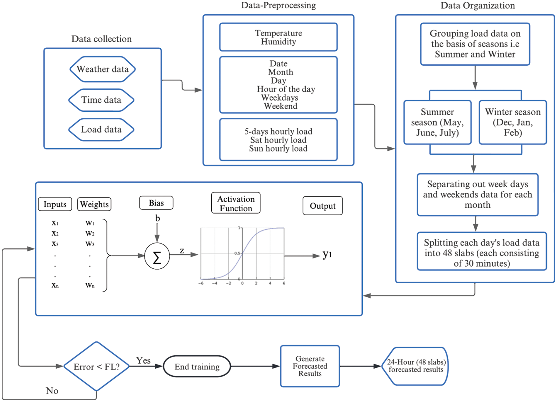
Figure 1: Proposed LM-based ANN system model

For accurate load forecasting, data is first fed to the preprocessing phase for cleaning purposes. The preprocessed data is inputted into the data classification phase to separate the load data into winter and summer seasons. Further, it is divided into weekends and weekdays, with each day’s data sliced into 48 splits. Next, the output of the data classification phase is passed to the proposed LM-based ANN model for training. We use an adaptive learning algorithm to train the model and use past load data for training to find the best possible weights. Afterward, the trained model is verified, and the next day’s load demand is forecasted for a very short period, i.e., thirty minutes. Following is the detail of each of these phases.

3.1 Dataset Description

We have used the USA power industry’s publicly available electrical hourly load dataset1 1https://www.eia.gov/. The period of the dataset used in this work is from January 1, 2019, to December 31, 2021. The dataset comprises 50,784 samples, each consisting of seven attributes (i.e., load, time, temperature, humidity, sunrise, sunset, and holiday). The ratio for the training dataset is 70% of the total dataset, and the remaining 30% is used for validation and testing. Data samples from January 2019 to September 2021 are taken for training, and load samples from October 2021 are used to evaluate the model’s perdition accuracy.

3.2 Data Preprocessing

The load profile for weekdays and weekends differs significantly; therefore, a separate analysis is conducted for weekdays and weekends. Data is processed on a daily, 5-days, and week-by-week basis. Since the load demand for any given hour of the day is like previous days’ loads, thus, the LM-based ANN model is trained on the historical load data. The data is preprocessed to obtain accurate forecasts after training. There is a strong association between data appropriateness and convergence of the model, i.e., the more the data is finetuned, the early the model will converge. Therefore, data is first fed to the cleaning phase, replacing the faulty and missing fields with the average values of the previous days’ load data. As electric load data always contain outliers, thus, normalization follows the cleaning phase to limit the weighted sum within the bounds of the activation function.

3.3 Data Organization

For best prediction results, dataset organization is carried out according to the following criteria.

•   Load data is first organized based on seasons, i.e., grouping into summer and winter. The winter season is spread over three months, i.e., December, January, and February, whereas the summer comprises May, June, and July. The remaining months have the usual load demands.

•   Each month’s load data is further separated into weekdays (5 working days) and weekends (Saturday and Sunday). Working days and weekends are worked separately as the load demand for weekends is less than for working days. Thus, weekend load data is not used to forecast load demand for working days and vice versa. We worked on weekly five days load data to predict next week’s working days load forecast.

•   Considering the fluctuating criticality of the load demand, each hourly load sample is divided into two equal halves, with each half containing the load data for half-hour. It helps predict STLF more precisely and accurately for a short period.

3.4 The Proposed LM-Based ANN Model Architecture

The proposed model uses multilayer perceptron (MLP) architecture with two layers, i.e., a hidden layer and an output layer, as described in Table 1. It is a feedforward neural network where the set of Pn inputs from the input layer are multiplied to weights wn, connected with each unit of a single hidden layer, which is connected to the output layer. The weighted summation X is described in Eq. (1).

X=P1w1+P2w2+…+Pnwn=∑n=1k⁡Pnwn(1)

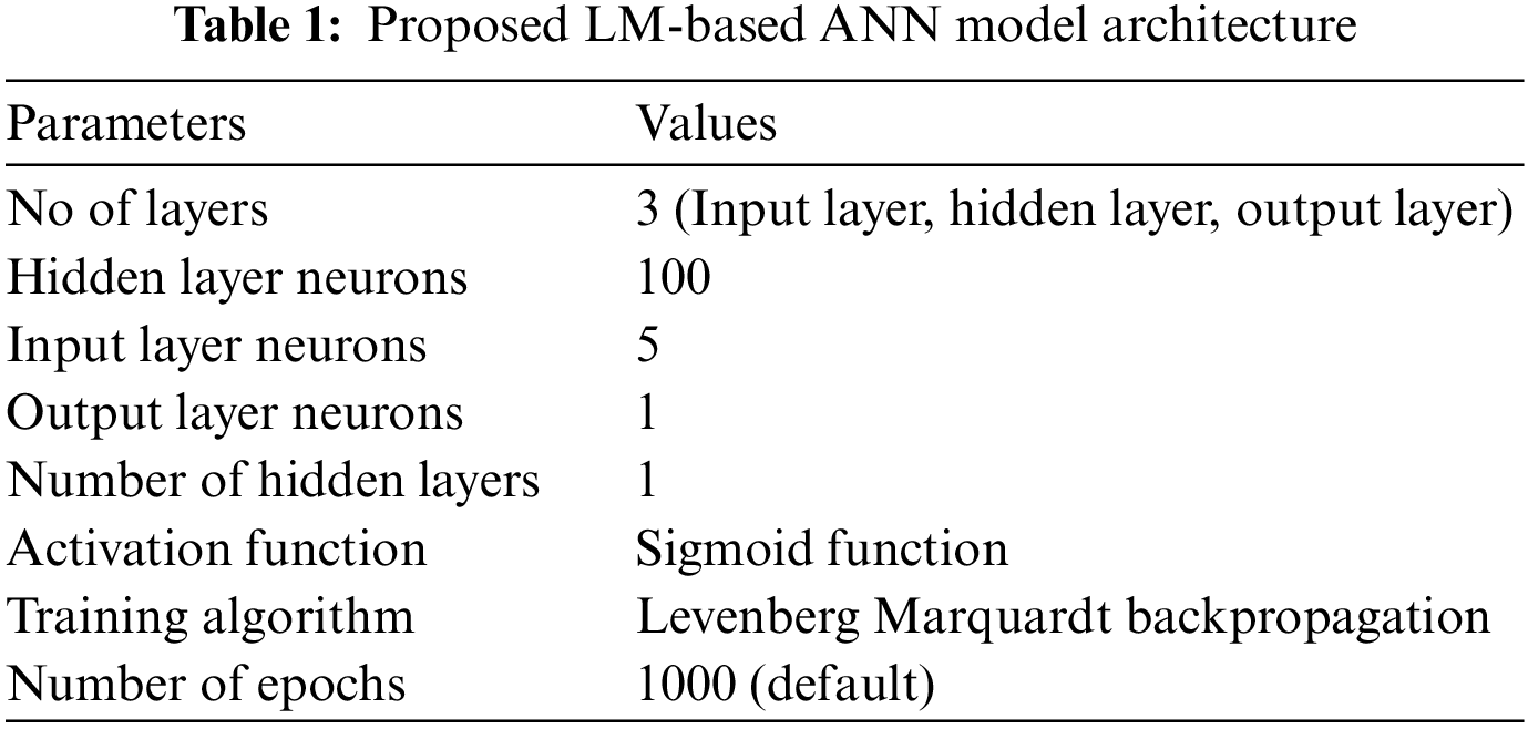
An activation function is used to achieve the desired outputs from the hidden layer. The activation function is required to be nondecreasing and differentiable for accurate training of ANNs. Thus, the log-sigmoid function f(X), is applied on weighted summation X at the hidden layer of our proposed LM-based ANN model and calculated as follows.

f(X)=1(1+e−X)(2)

The Purelin transfer function is used as an activation function at the output layer, which is a linear transfer function that calculates a layer’s output from its net input.

The proposed model uses the Levenberg-Marquardt (LM) backpropagation algorithm, one of the best optimization functions with a better learning rate than the other functions available for forecasting. The LM algorithm was designed by Hagan et al. [35] to address the shortcomings of gradient descent and the Gauss-Newton (GN) method. GN method converges very fast due to its quadratic properties, but it depends on initial weight values. In contrast, predicting suitable initial values in real-world problems is impossible. Similarly, gradient descent algorithms typically have a slow convergence speed. However, LM combines the benefits of both algorithms to present a hybrid optimization mechanism, making it appropriate for most prediction problems.

Initially, the model uses default values for the number of epochs and learning rate, which are adjusted later for model convergence during training. Moreover, the predicted load output is compared to the actual load data for performance evaluation, and different performance metrics have been applied. First, we calculated the mean absolute percentage error (MAPE) to check the accuracy of the proposed approach, which is defined as follows.

MAPE=1N∑t=1N⁡|Lt−FtLt|×100%(3)

In Eq. (3), Lt is the actual load at time t, N is the number of samples (48-time slabs for 24 h load forecast) and Ft is the forecasted load at time t.

The second performance metric is the root mean squared error (RMSE), a performance assessment indicator that estimates the errors of the predicted load forecast. It is defined as follows.

RMSE=1N∑t=1N⁡(Lt−Ft)2(4)

where Lt, is the actual load at time t, N is the number of samples, and Ft, is the forecasted load at time t.

The third performance metric is regression analysis, where we calculated the values of R2 and R. R2, also called goodness of fit, which measures the extent that variability in the actual load is explained by variability in the forecasted load values. At the same time, R measures the correlation between actual and forecasted load demand. The formulae for R2 and R are as follows:

R2=1−∑t=1N(Lt−Ft)2∑t=1N(Lt−F¯t)2(5)

where F¯t, is the mean value of the forecasted load Ft, at time t with the actual load Lt. When the values of R2 and R are closer to 1, it indicates the high accuracy of forecasted results.

R=±R2(6)

3.5 Training Process

In the model’s training process, we used the predictor and target datasets for training. The actual load values for a specific predictor dataset make up the target dataset. The training algorithm tries to minimize the difference between the expected output and actual output (loss function) and settles the weights and biases accordingly. The training goal is set at 0 to ensure zero tolerance for loss function. The training progresses to minimize the loss and enable the model to forecast the electric load accurately. The weights and biases are updated using backpropagation to reduce loss function.

Further, the movement of the error signal back to the input layer through the hidden layer can be generalized through the delta rule. The loss minimization procedure is repeated on an epoch-by-epoch basis until the model converges to a minimum or some stopping criteria meets, e.g., the total number of epochs. Initially, the number of epochs is 1000 (default value), which is later reduced to a maximum of 7 due to the early convergence of the model. An epoch is a comprehensive depiction of the ideal training regimen. The training procedure permits the LM-based ANN model to learn the relationship between inputs and outputs. It keeps learned information in the parametric form so that model can perform subsequent operations without retraining.

3.6 Optimization

The model is trained to provide desired outputs using historical data as input signals. Typically, every input after some processing generates an output signal in a system. The ultimate goal of the model is optimization, i.e., to minimize the loss function. Thus, the Levenberg Marquardt (LM) backpropagation algorithm is employed to get the desired output by iteratively modifying the internal weight and bias parameters of the ANN hidden layer. Initially, these parameters are given random values, and the sum of square error Єn is used to compute the network error from the initial parameters according to the following equation.

Єn=12∑1≤p≤P1≤k≤Krp,k2(7)

In the above equation, rp,k is training error with P is the total number of patterns and k is the total number of outputs. rp,k can be calculated as follows.

rp,k=Yp,k−Y^p,k(8)

where Yp,k and Y^p,k are the actual and predicted values of the kth output and pth pattern, respectively. Afterward, the LM algorithm updates the weights parameters by using the following equation.

wn+1=wn−(Ҥ)−1JЄn(9)

In the above equation, wn+1 is the value of the updated weight and wn is the prior value of weights, and J is the Jacobian matrix that contains the first derivatives of network error with respect to weights. Ҥ is the Hessian matrix that can be expressed as:

Ҥ=JTJ+(μI)(10)

where I is the unity matrix and μ is the combination coefficient. When coefficient μ is zero, it reduces to just Newton’s method. Newton’s method is more efficient and faster; thus, it tried to move toward newton’s method as rapidly as possible. Therefore, it is intended to decrease μ′s value in every step. LM consider μ′s value only when updated error Єn+1 value is smaller than current Єn value. If updated error Єn+1 gets a larger value than prior Єn, then the process will be restarted from the first step of initial random weights initialization [36,37]. The systematic flow of the LM algorithm is described in Fig. 2.

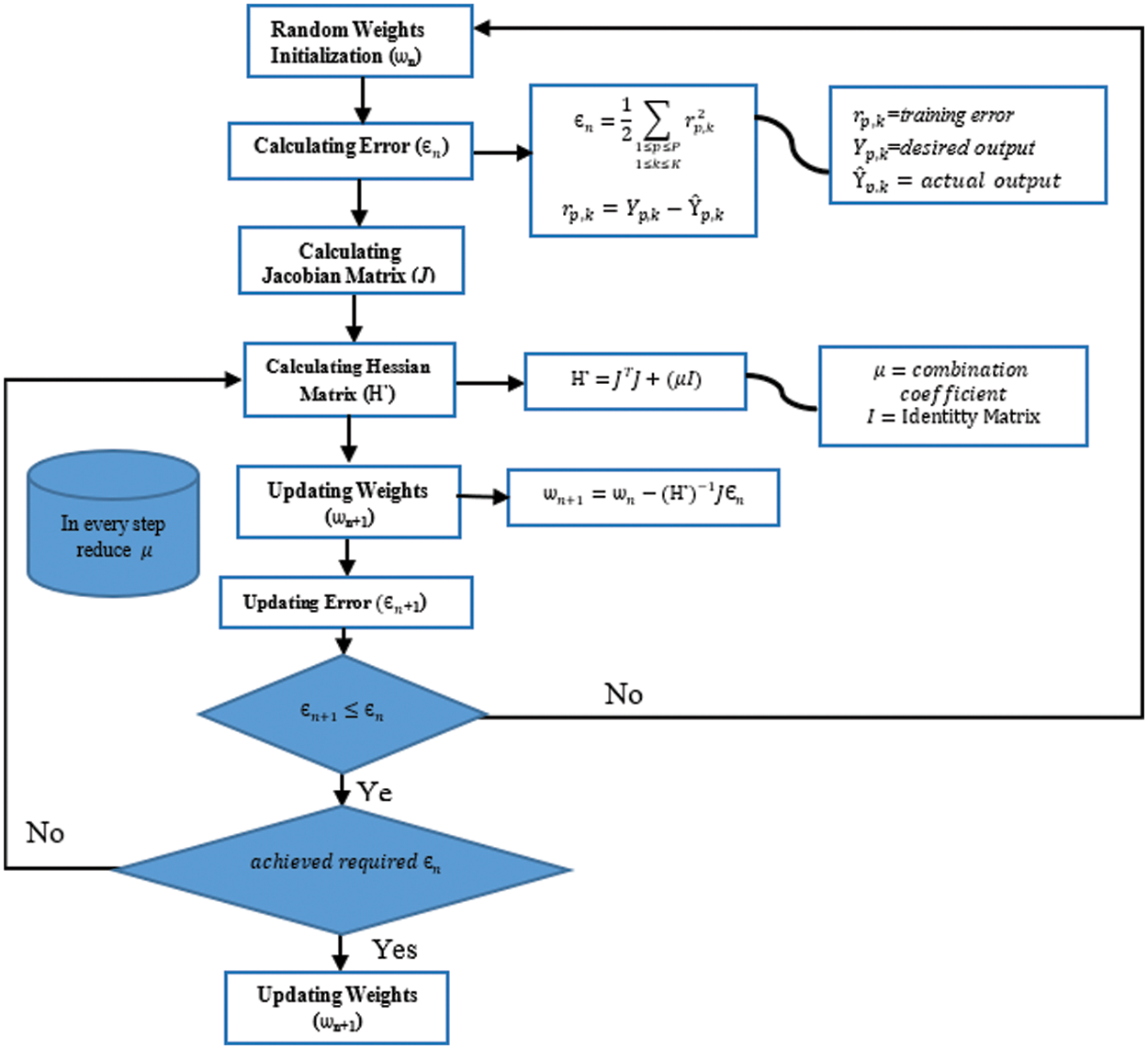
Figure 2: Workflow of Levenberg–Marquardt algorithm

Finally, validation and testing followed the training. After the network has been trained, it is put to the test by feeding it test load forecast data. The anticipated load output is compared to the actual load output to calculate the inaccuracy.

4  Results and Discussion

The proposed LM-based ANN model is empowered with training to forecast future load demands with acceptable accuracy. The results for the winter and summer seasons are obtained separately, with the summer season consisting of May, June, and July, while the winter season comprises December, January, and February. Moreover, the load demand within a month is forecasted separately for weekdays and weekends. Further, each day is sliced into 48 slabs to predict STLF for a very short period. Afterward, the following performance metrics are calculated to evaluate the model’s performance.

4.1 Regression Analysis

The regression analysis determines the values of R2 and R to measure the goodness of fit and correlation between actual and predicted load demand of the proposed model on test data. Fig. 3 shows the plots for May, June, and July, depicting the regression analysis for the summer season. Similarly, Fig. 4 shows the plots for December, January, and February describing the regression analysis for the winter season. In each regression plot, the solid line is the best-fit line indicating the linear regression between outputs and targets. The light-colored band represents the 95% confidence band, while the dark band represents the 95% prediction band denoting the relationship between the actual and predicted load demand.

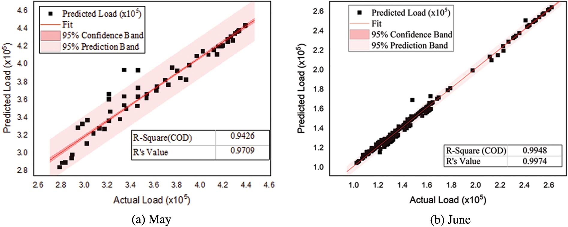
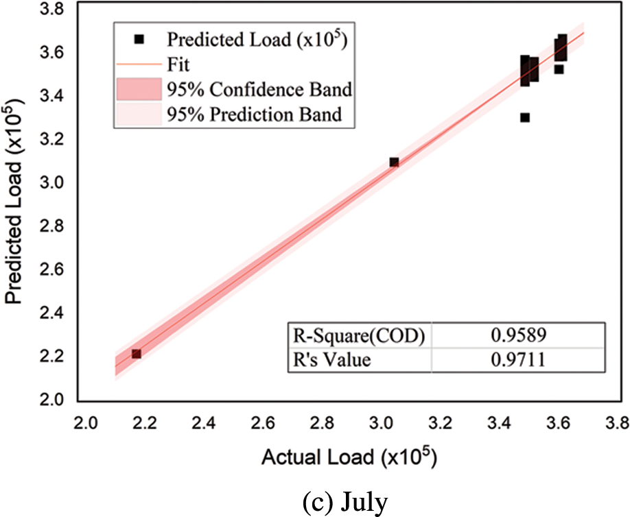
Figure 3: Regression analysis (predicted vs. actual load) for the summer season

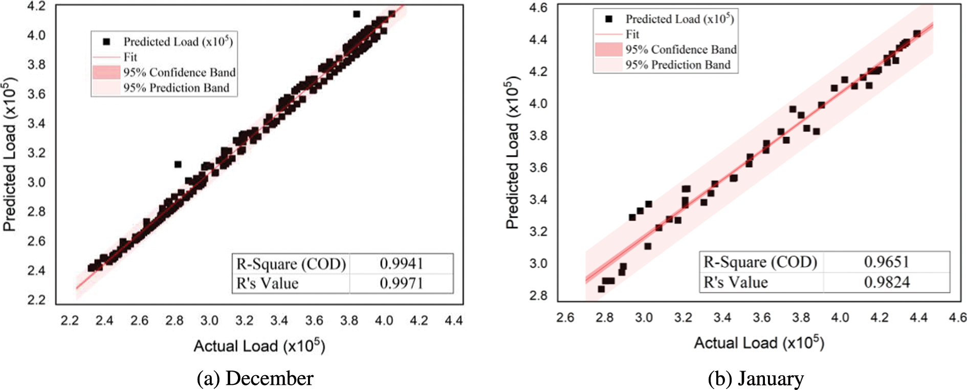
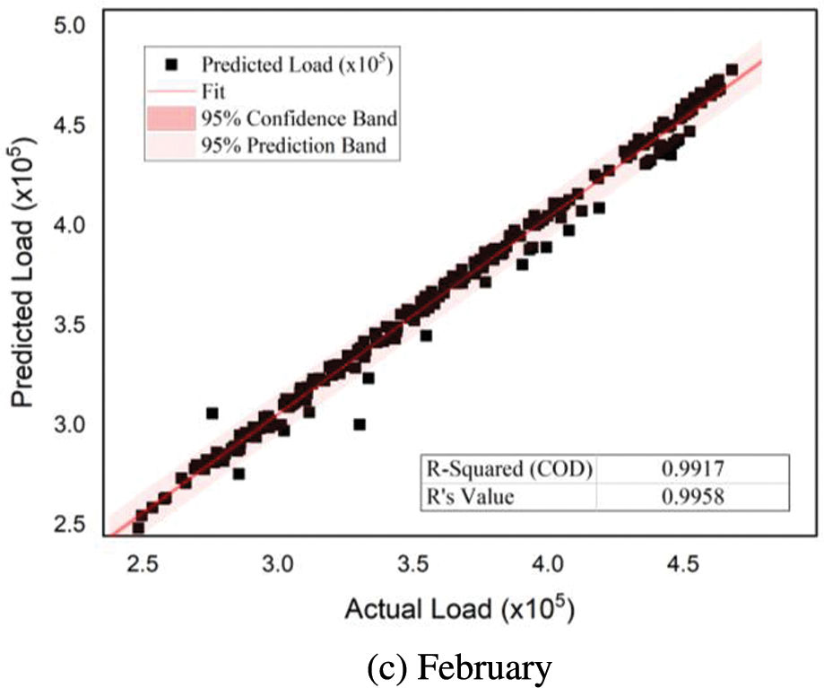
Figure 4: Regression analysis (predicted vs. actual load) for the winter season

All these plots estimate the accuracy with which the trained model forecasts the future load. These plots also depict the model’s capacity to learn the complex relationship between historical load demand, weather, and time data for accurate load forecasts. In each plot of Figs. 3 and 4, the values R2 and R are calculated; the closer the value of R2 to 1, the more accurate the model results are. Similarly, R = 1 indicates an exact linear relationship between actual and predicted load, whereas its close to zero value means no linear relationship. It is seen that for all months of the summer and winter seasons, R2 and R values are close to 1, leading to an excellent response and validating the proposed model’s accuracy.

4.2 Error Evaluation (RMSE and MAPE)

Another way to represent the model’s performance on training and testing datasets is to measure the error rate across varying epochs. The model training is poor when there is high variance and bias. It indicates that the model is storing training dataset information instead of learning. High bias signifies a high rate of error during training and testing, whereas high variance indicates the noticeable gap between the prediction accuracy of training and testing of the model. In either case, the model performs poorly and results in vague generalization. Another problem is overfitting, which occurs when a model performs well in training but does not show good performance on testing. Such a model memorizes the dataset parameters instead of learning from them, leading to a lousy generalization.

Table 2 depicts the performance measure of the proposed LM-based ANN model, demonstrating the relation among RMSE, MAPE, and the number of epochs for the different months of the summer and winter seasons. It also shows a set of experimented network parameters and their results. The model is tested with varying sets of hyperparameters, i.e., the number of neurons used at the hidden layer, the number of hidden layers, the choice of transfer functions used at each layer, model architecture, training and learning functions, etc. A trial-and-error approach is investigated with the model until the best set is attained. It can be seen that with the increased number of neurons at the hidden layer, the model gets improved RMSE and MAPE results.

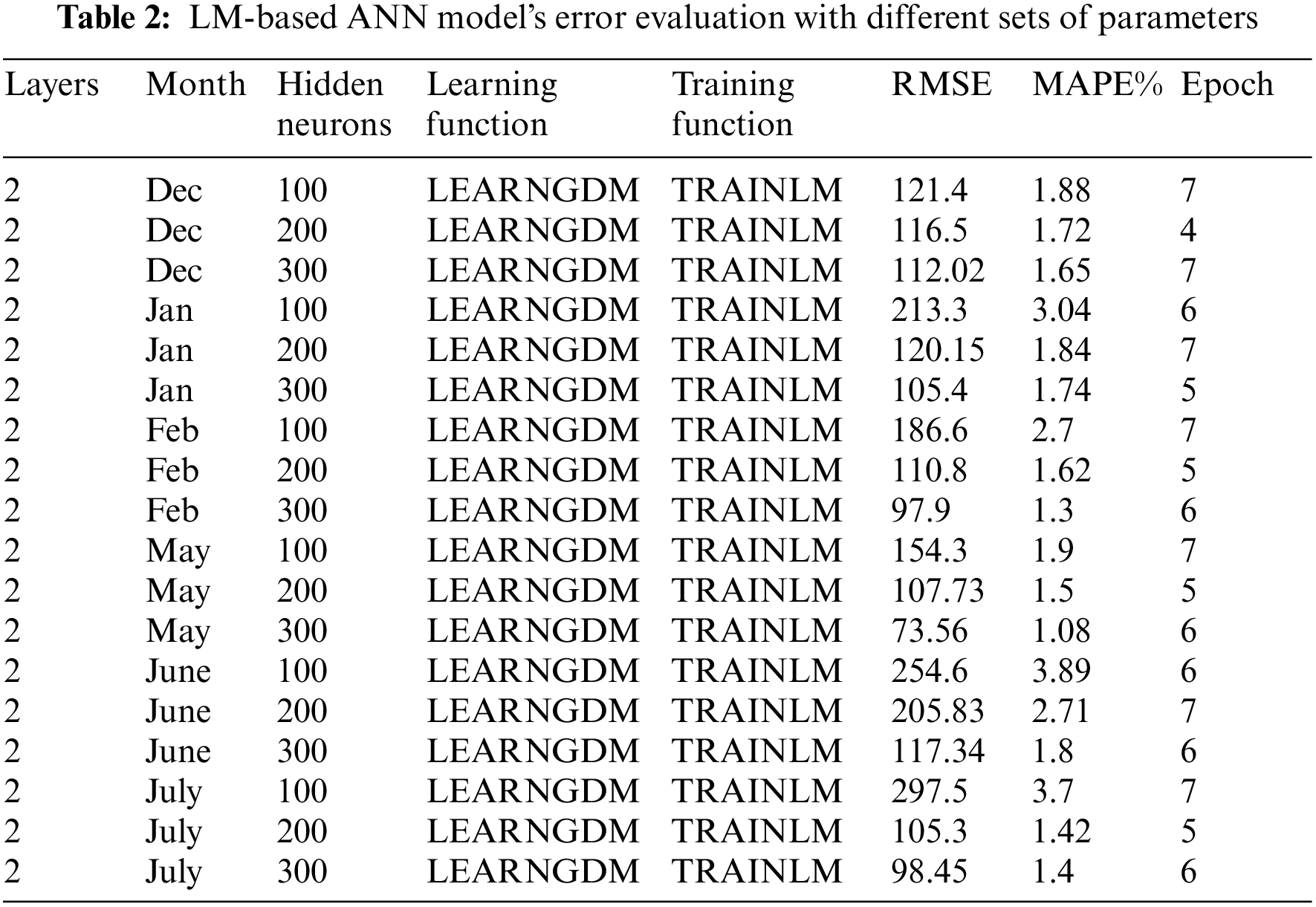
Similarly, the log-sigmoid transfer function turns out to be good, giving better RMSE and MAPE values than the tan-sigmoid function used at the hidden layer neurons of the LM-based ANN model. It is also observed that the size of the dataset also contributes to the model’s performance, i.e., the larger the size of the dataset, the better the model’s performance. The table shows that the model gets the best results at very early epochs. Thus, our proposed LM-based ANN model resolved the problem of overfitting. Moreover, from the empirical results, it can be concluded that the network is trained to forecast with high accuracy.

4.3 Forecasted and Actual Results Evaluation

The ultimate goal of this paper is to forecast the next day’s load with maximum accuracy. For which the LM-based ANN model is trained using the best hyperparameter values and optimized weights that give the best prediction results for the target load data. Finally, the best hyperparameter values of the model training are documented, and the model is tested with test data to check its prediction performance on unseen data.

Fig. 5 shows the difference between the forecasted load and actual load demand for 1st five weekdays, with each day sliced into 48 slabs (total of 240 slabs) during different months of the summer season. Similarly, Fig. 6 shows the difference between the forecasted load and actual load demand for 1st five weekdays during different months of the winter season. The plots of both figures depict that the forecasted load is very close to the actual load demand. Thus, our proposed LM-based ANN model is robust enough to predict STLF for the next week.

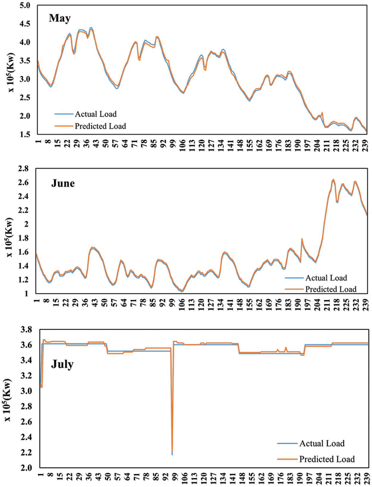
Figure 5: Load forecast plots for weekdays during months of the summer season

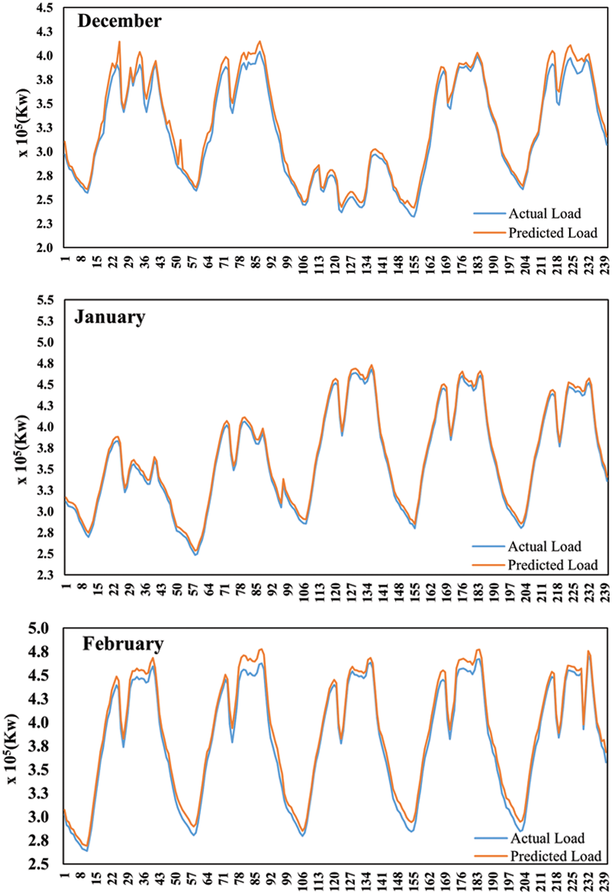
Figure 6: Load forecast plots for weekdays during months of the winter season

4.4 Comparison with Other Techniques

We forecasted the load for the next day, with each day sliced into 48 slabs bearing maximum accuracy. Compared with other state-of-the-art machine learning techniques [19,33,36], which forecasted the load for the next day and the next hour, we predicted the load for the next thirty minutes with comparable high accuracy. It makes the load prediction according to the need of the hour for the power system enabling them to generate load according to the forecast for a very short period. Moreover, in [33], their RMSE and R values are for the whole summer or winter season, whereas we calculated the result for every month for MAPE and R performance metrics with almost identical best scores. Though they forecasted the hour-ahead load, they depicted it for a whole day. Thus, it is difficult to consider it as an hour-ahead prediction, whereas we calculated the load forecast for every thirty minutes (240 slabs) and depicted it graphically very clearly. Thus, it can be concluded that our LM-based ANN model outperforms the state-of-the-art techniques for predicting load for a very short period with comparable high accuracy and the lowest error rates.

5  Conclusion

Power load prediction is essential for an effective energy system operation and scheduling. This paper proposed an LM-based ANN model to forecast short-term electricity load. We collected the USA Power Industry’s electric load dataset for model training from 2019 to 2021. Weekdays and weekends are separated for the winter and summer seasons, considering the significant variation of load demands for different seasons as well as for weekends and weekdays. Owing to the dynamic and temporal nature of the load profile, each day’s load is further divided into 48 slabs, each consisting of 30 min. We take time and weather data with historical load demand simultaneously as input to the LM-based ANN model due to the great impact of meteorological parameters on the next day’s load demand. The Levenberg-Marquardt optimization technique is used as a backpropagation algorithm in the LM-based ANN model to optimize its performance. The model’s performance is evaluated using statistical measures, i.e., RMSE, MAPE, R, R2. The RMSE and MAPE give lower error rates, whereas R2 and R produce optimal values that prove the robustness of the LM-based ANN model. The empirical results show that the proposed electric load forecasting model outperforms in terms of forecast accuracy with the lowest error rates.

Although the LM-based ANN model is robust in processing time series data, its parameters still have some room for optimization (i.e., finetuning of significant parameters) to improve the computing efficiency. Moreover, forecasting accuracy can be further enhanced by considering other important factors, such as locations, social variables, etc. Our future work will investigate other deep learning-based forecasting mechanisms like convolutional neural networks and recurrent neural networks to deal with more complex and larger datasets.

Funding Statement: The authors acknowledge the financial support provided in part by the National Key Research and Development Program of China (No.2020YFB1005804), in part by the National Natural Science Foundation of China under Grant 61632009, in part by the High-Level Talents Program of Higher Education in Guangdong Province under Grant 2016ZJ01, and in part by the NCRA-017, NUST, Islamabad.

Conflicts of Interest: The authors declare that they have no conflicts of interest.

References

1. S. Bhattacharya, R. Chengoden, G. Srivastava, M. Alazab, A. R. Javed et al., “Incentive mechanisms for smart grid: State of the art, challenges, open issues, future directions,” Big Data and Cognitive Computing, vol. 6, no. 2, pp. 1–28, 2022. [Google Scholar]
2. M. Alazab, S. Khan, S. S. R. Krishnan, Q. V. Pham, M. P. K. Reddy et al., “A multidirectional LSTM model for predicting the stability of a smart grid,” IEEE Access, vol. 8, no. 4, pp. 85454–85463, 2020. [Google Scholar]
3. N. Ahmad, Y. Ghadi and S. Member, “Load forecasting techniques for power system : Research challenges and survey,” IEEE Access, vol. 10, no. 7, pp. 71054–71090, 2022. [Google Scholar]
4. G. Hafeez, K. S. Alimgeer and I. Khan, “Electric load forecasting based on deep learning and optimized by Heuristic algorithm in smart grid,” Applied Energy, vol. 269, pp. 1–18, 2020. [Google Scholar]
5. D. M. Teferra, L. M. H. Ngoo and G. N. Nyakoe, “Fuzzy-swarm intelligence-based short-term load forecasting model as a solution to power quality issues existing in microgrid system,” Journal of Electrical and Computing Engineering, vol. 2022, pp. 1–14, 2022. [Google Scholar]
6. A. Rahman, V. Srikumar and A. D. Smith, “Predicting electricity consumption for commercial and residential buildings using deep recurrent neural networks,” Applied Energy, vol. 212, pp. 372–385, 2018. [Google Scholar]
7. K. G. Boroojeni, M. H. Amini, S. Bahrami, S. S. Iyengar, A. I. Sarwat et al., “A novel multi-time-scale modeling for electric power demand forecasting: From short-term to medium-term horizon,” Electric Power Systems Reserach, vol. 142, pp. 58–73, 2017. [Google Scholar]
8. Y. Li, J. Che and Y. Yang, “Subsampled support vector regression ensemble for short term electric load forecasting,” Energy, vol. 164, pp. 160–170, 2018. [Google Scholar]
9. S. Taheri, B. Talebjedi and T. Laukkanen, “Electricity demand time series forecasting based on empirical mode decomposition and long short-term memory,” Energy Engineering: Journal of the Association of Energy Engineering, vol. 118, no. 6, pp. 1577–1594, 2021. [Google Scholar]
10. M. Irfan, A. Raza, F. Althobiani, N. Ayub, M. Idrees et al., “Week ahead electricity power and price forecasting using improved DenseNet-121 method,” Computers, Materials & Continua, vol. 72, no. 3, pp. 4249–4265, 2022. [Google Scholar]
11. A. Alrashidi and A. Mustafa Qamar, “Data-driven load forecasting using machine learning and meteorological data,” Computer Systems Science and Engineering, vol. 44, no. 3, pp. 1973–1988, 2023. [Google Scholar]
12. A. K. Bashir, S. Khan, B. Prabadevi, N. Deepa, W. S. Alnumay et al., “Comparative analysis of machine learning algorithms for prediction of smart grid stability,” International Transactions on Electrical Energy Systems, vol. 31, no. 9, pp. 1–23, 2021. [Google Scholar]
13. H. Jiang, Y. Zhang, E. Muljadi, J. J. Zhang and D. W. Gao, “A Short-term and high-resolution distribution system load forecasting approach using support vector regression with hybrid parameters optimization,” IEEE Transactions on Smart Grid, vol. 9, no. 4, pp. 3341–3350, 2018. [Google Scholar]
14. F. Zhu and G. Wu, “Load forecasting of the power system: An investigation based on the method of random forest regression,” Energy Engineering: Journal of the Association of Energy Engineering, vol. 118, no. 6, pp. 1703–1712, 2021. [Google Scholar]
15. N. Abu-Shikhah, F. Elkarmi and O. M. Aloquili, “Medium-term electric load forecasting using multivariable linear and non-linear regression,” Smart Grid and Renewable Energy, vol. 2, no. 2, pp. 126–135, 2011. [Google Scholar]
16. S. Siami-Namini, N. Tavakoli and A. Siami Namin, “A comparison of ARIMA and LSTM in forecasting time series,” in Proc.—17th IEEE Int. Conf. on Machine Learning and Applications, ICMLA, Orlando, Florida, USA, pp. 1394–1401, 2019. [Google Scholar]
17. J. Zhu, H. Dong, W. Zheng, S. Li, Y. Huang et al., “Review and prospect of data-driven techniques for load forecasting in integrated energy systems,” Applied Energy, vol. 321, pp. 119269, 2022. [Google Scholar]
18. N. A. Mohammed and A. Al-Bazi, “An adaptive backpropagation algorithm for long-term electricity load forecasting,” Neural Computing and Applications, vol. 34, no. 1, pp. 477–491, 2022. [Google Scholar]
19. P. H. Kuo and C. J. Huang, “A high precision artificial neural networks model for short-term energy load forecasting,” Energies, vol. 11, no. 1, pp. 1–13, 2018. [Google Scholar]
20. K. Chen, K. Chen, Q. Wang, Z. He, J. Hu et al., “Short-term load forecasting with deep residual networks,” IEEE Transactions on Smart Grid, vol. 10, no. 4, pp. 3943–3952, 2019. [Google Scholar]
21. S. M. Elgarhy, M. M. Othman, A. Taha and H. M. Hasanien, “Short term load forecasting using ANN technique,” in 2017 19th Int. Middle-East Power Systems Conf. MEPCON 2017—Proc., Cairo, Egypt, pp. 1385–1394, 2018. [Google Scholar]
22. S. Hosein and P. Hosein, “Load forecasting using deep neural networks,” in 2017 IEEE Power & Energy Society Innovative Smart Grid Technologies Conf. (ISGT), Torino, Italy, pp. 1–5, 2017. [Google Scholar]
23. G. M. U. Din and A. K. Marnerides, “Short term power load forecasting using deep neural networks,” in 2017 Int. Conf. on Computing, Networking and Communications (ICNC), Silicon Valley, California, USA, pp. 594–598, 2017. [Google Scholar]
24. Z. Guo, K. Zhou, X. Zhang and S. Yang, “A deep learning model for short-term power load and probability density forecasting,” Energy, vol. 160, pp. 1186–1200, 2018. [Google Scholar]
25. T. Hossen, A. S. Nair, R. A. Chinnathambi and P. Ranganathan, “Residential load forecasting using deep neural networks (DNN),” in 2018 North American Power Symp. (NAPS), Fargo, North Dakota, USA, pp. 1–5, 2018. [Google Scholar]
26. T. Hossen, S. J. Plathottam, R. K. Angamuthu, P. Ranganathan and H. Salehfar, “Short-term load forecasting using deep neural networks (DNN),” in 2017 North American Power Symp. (NAPS), Morgantown, West Virginia, USA, pp. 1–6, 2017. [Google Scholar]
27. T. Ciechulski and S. Osowski, “High precision lstm model for short-time load forecasting in power systems,” Energies, vol. 14, no. 11, pp. 1–15, 2021. [Google Scholar]
28. D. Zhang, H. Tong, F. Li, L. Xiang and X. Ding, “An ultra-short-term electrical load forecasting method based on temperature-factor-weight and LSTM model,” Energies, vol. 13, no. 18, pp. 1–14, 2020. [Google Scholar]
29. W. Kong, Z. Y. Dong, Y. Jia, D. J. Hill, Y. Xu et al., “Short-term residential load forecasting based on LSTM recurrent neural network,” IEEE Transactions on Smart Grid, vol. 10, no. 1, pp. 841–851, 2019. [Google Scholar]
30. R. Eapen and S. Simon, “Performance analysis of combined similar day and day ahead short term electrical load forecasting using sequential hybrid neural networks,” IETE Journal of Reserach, vol. 65, no. 2, pp. 216–226, 2019. [Google Scholar]
31. J. Zhang, Y. M. Wei, D. Li, Z. Tan and J. Zhou, “Short term electricity load forecasting using a hybrid model,” Energy, vol. 158, pp. 774–781, 2018. [Google Scholar]
32. M. R. Haq and Z. Ni, “A new hybrid model for short-term electricity load forecasting,” IEEE Access, vol. 7, no. 8, pp. 125413–125423, 2019. [Google Scholar]
33. M. J. A. Shohan, M. O. Faruque and S. Y. Foo, “Forecasting of electric load using a hybrid LSTM-neural prophet model,” Energies, vol. 15, no. 6, pp. 1–18, 2022. [Google Scholar]
34. M. Massaoudi, S. S. Refaat, I. Chihi, M. Trabelsi, F. S. Oueslati et al., “A novel stacked generalization ensemble-based hybrid LGBM-XGB-MLP model for short-term load forecasting,” Energy, vol. 214, pp. 1–14, 2021. [Google Scholar]
35. M. T. Hagan and M. B. Menhaj, “Training feedforward networks with the Marquardt algorithm,” IEEE Transactions on Neural Networks, vol. 5, no. 6, pp. 989–993, 1994. [Google Scholar]
36. Q. H. Giap, D. L. Nguyen, T. T. Q. Nguyen and T. M. D. Tran, “Applying neural network and Levenberg–Marquardt algorithm for load forecasting in IA-Grai district, Gia Lai Province,” Journal of Science and Technology: Issue on Information and Communications Technology, vol. 20, no. 6, pp. 13–18, 2022. [Google Scholar]
37. Y. C. Du and A. Stephanus, “Levenberg-Marquardt neural network algorithm for degree of arteriovenous fistula stenosis classification using a dual optical photoplethysmography sensor,” Sensors, vol. 18, no. 7, pp. 1–18, 2018. [Google Scholar]
Cite This Article
Copyright © 2023 The Author(s). Published by Tech Science Press.
This work is licensed under a Creative Commons Attribution 4.0 International License , which permits unrestricted use, distribution, and reproduction in any medium, provided the original work is properly cited.
Downloads
Citation Tools