A WSN Node Fault Diagnosis Model Based on BRB with Self-Adaptive Quality Factor

1  Introduction

A wireless sensor network (WSN) is a physical system for data collection that is often placed in remote areas to collect data [1], such as deep forests, high altitudes, and underwater environments. Now that WSNs work in harsh environments, as the working hours of sensor nodes increases and the impact of the wireless communication environment, the possibility of node failure increases [2]. To grasp the WSN’s working status in time and ensure the reliability of the collected data, WSN node fault diagnosis is essential [3].

Commonly used WSN node fault diagnosis methods are neural network methods, decision tree methods, and random forest methods [4–7]. Among them, neural network methods are the most widely used. WSN node fault diagnosis requires the extraction of data features. However, the data features are not entirely reliable due to the harsh working environments and the interference of wireless signal transmission. However, the above methods do not consider the impact of unreliable data features on the WSN node fault diagnosis process. These unreliable data may lead to anomalous training of the parameters in the method, reducing fault diagnosis accuracy. Meanwhile, most of the above methods are data-driven, with parameters requiring many uniform fault samples to train the parameters for better diagnostic accuracy. However, in actual industrial production, the number of failure samples is small and unlikely to be uniform, which significantly limits the diagnostic accuracy of the data-driven methods.

This paper proposes a WSN node fault diagnosis method based on a belief rule base (BRB) with a self-adaptive quality factor (BRB-SAQF) to solve the above existing problems. The method has two advantages. First, the concept of the quality factor is introduced to reduce the influence of unreliable data. In addition, because BRB is less dependent on the number of training samples and this method is combined with the parameter setting by expert knowledge, which requires fewer fault samples than the data-driven methods. Therefore, good diagnostic results can also be achieved when the number of fault samples is small. To verify the validity of the BRB-SAQF, it is compared with other approaches, such as artificial neural networks, Gaussian regression processes, support vector machines, decision trees and boosting trees.

Through a case study and comparison with the commonly used fault diagnosis methods, it can be concluded that the BRB-SAQF method can effectively reduce the influence of unreliable data on fault diagnosis accuracy. Compared with the data-driven methods, the BRB-SAQF method can also achieve better diagnosis results with the same data samples, and its effectiveness is proven in this paper.

The rest of the article is then structured as follows. Section 2 introduces the current research status of WSN node fault diagnosis and the advantages of the proposed method proposed in this paper. Section 3 defines the problems encountered during the troubleshooting of WSN nodes, and the model’s basic structure is illustrated. Section 4 presents the data feature extraction methods, attribute quality factor calculation, model inference process and parameter optimization. In Section 5, the effectiveness of the fault diagnosis method proposed in this paper is verified through a case study. Section 6 summarizes the fault diagnosis method proposed in this paper, and subsequent research work is discussed.

2  Related Work

Due to the widespread use of WSNs, fault diagnosis and classification of WSN nodes have become research topics for related scholars. For example, Saeed et al. proposed a WSN node fault diagnosis method based on supervised learning and integrated learning schemes for extremely random trees [5]. Noshad et al. used a random forest approach to diagnose faults in WSNs [6]. Swain et al. proposed an automatic fault diagnosis model using a hybrid metaheuristic algorithm to train feedforward neural networks for WSN node fault diagnosis [8]. Gharamaleki et al. determined the failure of a WSN by the variability of neighboring nodes [9]. Mohapatra et al. used neural networks to simulate the process of human immunity to achieve WSN node fault diagnosis [10]. Regin et al. used a convolutional neural network approach for WSN node fault diagnosis [11]. It is easy to see that the most widely used methods for WSN node fault diagnosis are neural network-based methods [12,13].

However, whether it is a neural network-based method or related to the decision tree method, these fault diagnosis methods have three drawbacks. First, these methods do not consider the impact of unreliable data features on fault diagnosis accuracy. Second, they require many uniform fault samples to train the model parameters. Finally, neural network-based methods have a larger number of parameters, such as weights and biases of neurons, which do not have a specific physical meaning, and the interpretability of these methods is poor.

In 2006, Yang et al. proposed a belief rule base inference method based on an evidential reasoning approach (RIMER) [14]. Essentially, RIMER is an expert system consisting of belief rule base (BRB) and evidential reasoning (ER) rules that allow for a more flexible representation of various types of uncertain information, including ambiguity, randomness, and ignorance [15]. The model’s parameters are given by experts based on empirical knowledge and have a specific physical meaning in the model. Thus, BRB has the advantage of small sample training [16]. BRB is widely used in medical diagnosis, health status assessment, troubleshooting, etc., [17–20]. Therefore, He et al. proposed a fault diagnosis method for WSNs based on BRB [21]. However, the method also does not consider the effect of unreliable data features on the fault diagnosis process.

In 2018, a new BRB model with attribute reliability was proposed by Feng et al. [22]. When the concept of attribute reliability was introduced, a new static attribute reliability calculation method was proposed. However, the static attribute reliability calculation method does not apply to input attributes with significant variations in different states.

To reduce the impact of unreliable data features on the fault diagnosis process and to bridge the lack of static attribute reliability calculations, this paper proposes a BRB-SAQF-based node fault diagnosis model for WSNs. First, the concept of the attribute quality factor is introduced to mask part of the unreliable data to calculate the quality factors of each attribute. Second, the self-adaptive quality factor calculation method is rederived based on the static attribute reliability calculation method. Third, because BRB has the advantage of small sample training, the required number of the proposed method’s training samples is smaller than that of the neural network methods. Finally, the interpretability of the method is also more robust than that of the neural network methods because the settings of the BRB method parameters are determined by expert knowledge and have a specific physical meaning. The current methods of fault diagnosis and the solutions in this paper are represented in Fig. 1.

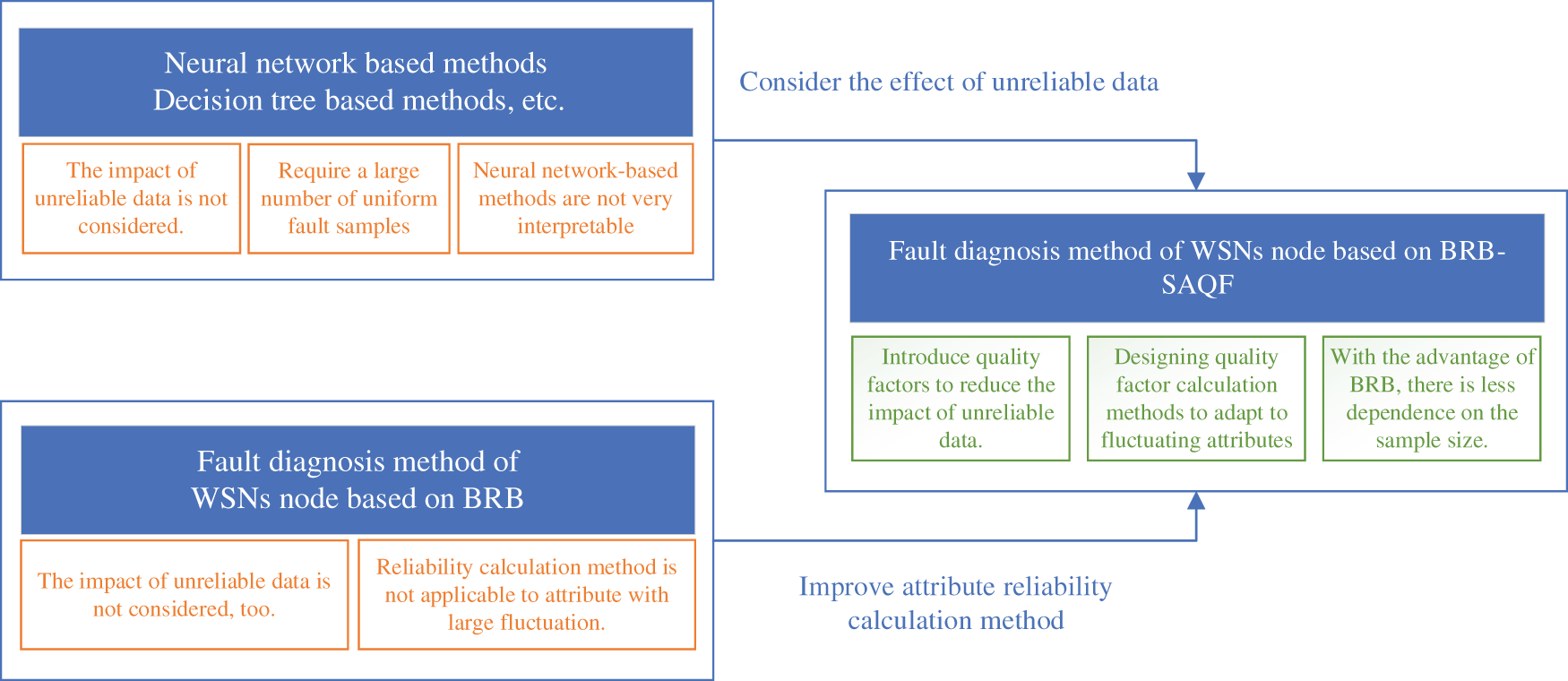
Figure 1: Problems with the current study and solution

3  Problem Formulation and Basic Structure of the Model

In this section, some of the problems encountered in the fault diagnosis process of the WSN node are defined, and the model’s basic structure is constructed based on these problems.

3.1 Problem Formulation

Problem 1: Several different data features must be extracted as input attributes for the BRB-SAQF model. The raw node data collected by the WSN can be used to determine whether a node is malfunctioning. However, it is impossible to decide what type of failure occurred in this node. Therefore, different data features must be extracted and used to distinguish the fault type of the node. Extracting data features can be described in Eq. (1).

[x1,x2,…,xM]=f(Xm,φ)(1)

where f() represents the extraction process of data features and Xm means the raw data collected by WSN sensors. The letter φ represents the parameters in the data feature extraction process. The vector [x1,x2,…,xM] represents M data features that are extracted.

Problem 2: The model needs to handle the unreliability of input attributes and define the attribute quality factor parameters. WSN works in a relatively harsh environment, and the data transmission process is often influenced by electromagnetic fields, temperature, humidity and other factors, resulting in noise in the observation data. As a result, the extracted data features contain errors, causing the data features to be incompletely reliable, i.e., the input attributes of the model are unreliable. Therefore, after data feature extraction, it is necessary to identify and deal with the errors caused by noise. The unreliability processing of input attributes can be expressed in Eq. (2).

[r1,r2,…,rM]=g([x1,x2,…,xM],γ)(2)

where g() represents the calculation function of the attribute quality factor and the vector [x1,x2,…,xM] represents the M data features extracted from Problem 1. γ represents the parameters in the attribute quality factor calculation process. The vector [r1,r2,…,rM] represents the quality factors of each input attribute.

Problem 3: The attribute quality factor must be incorporated into the BRB inference process. The quality factors of the input attributes are introduced as new parameters for the BRB method. Therefore, it is necessary to consider modifying the BRB’s original inference process to consider the attribute quality factors. The BRB inference process incorporating attribute quality factors can be described by Eq. (3).

S=h([r1,r2,…,rM],ρ)(3)

where [r1,r2,…,rM] represents the quality factors of the input attributes and ρ denotes other parameters in the fusion process. The symbol h() indicates the BRB-SAQF reasoning process. The alphabet S means the diagnostic result of the model.

Problem 4: The parameters initialized in the BRB-SAQF model must be optimized to obtain more accurate diagnostic results. The optimization process of the model’s parameters can be expressed by Eq. (4).

ηbest=o(η,ψ)(4)

where η represents parameters that need to be optimized. The symbol ηbest represents optimized parameters. The symbol ψ denotes the parameters of the optimization algorithm.

3.2 Basic Structure of the Model

According to the four problems above, the node fault diagnosis model of the WSN based on BRB-SAQF is divided into the following four parts. The first part is the data feature extraction unit, which extracts the data features from the original data that are beneficial to fault diagnosis. The second part is the calculation unit of the model input attribute quality factor, which calculates the attribute quality factor using the self-adaptive quality factor calculation method. The third part is the model rule construction and inference module, which initializes the rules in BRB-SAQF and implements the inference process considering the attribute quality factor. The fourth part is the optimization module of model parameters, which optimizes the initial parameters of the model to obtain better diagnostic results through the optimization algorithm with constraints. The basic structure of the model is shown in Fig. 2.

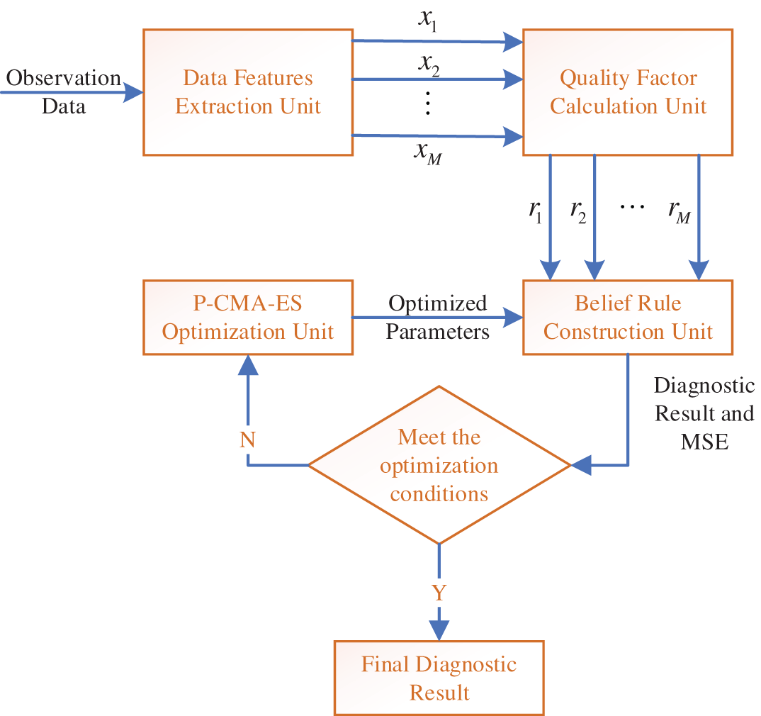
Figure 2: Components of the BRB-SAQF model

4  Construction of the WSN Node Fault Diagnosis Model Based on BRB-SAQF

In Section 3, we defined the critical problems in the node fault diagnosis process of WSNs based on the BRB-SAQF method. In this section, we propose solutions to each of these problems.

4.1 Extraction of Data Features

Different data features must be extracted from the observed data to distinguish what type of failure has occurred on a node. The standard data features used in the WSN node fault diagnosis process are the mean, standard deviation, variance, skewness and kurtosis [21]. This paper uses mean gap and kurtosis as the extracted data features for the discrimination of different fault types. Both of these data features belong to time-dependent feature data. The mean gap represents the distance between the mean value of the node being diagnosed and the mean value of its neighboring nodes over a period of time. Kurtosis is the characteristic number of the peak height of the probability density distribution curve at the mean [23]. The sensor observation data is defined as Xm(t), which can be described by Eq. (5).

Xm(t)=[x1(t),x2(t),…,xm(t)](5)

where xm(t) represents the data collected by m sensors at the moment t. Then, the mean gap from moment l to l+T can be calculated as Eq. (6).

gi=|∑t=ll+Txi(t)T+1−∑t=ll+T∑j=1mxj(t)m(T+1)|,i,j=1,…,m,i≠j(6)

where m denotes the number of proximate sensors. The kurtosis can be calculated by Eq. (7).

un=1T+1∑t=ll+T[xi(t)−x¯i]4σ4(7)

where T indicates the size of the time interval and x¯i denotes the average value of data collected by the sensor i during the time interval T. The expression σ4 represents the standard deviation of the data collected by the sensor i during the time interval T.

4.2 Calculating Attribute Quality Factors

When the BRB model considers attribute quality factors, calculating it becomes a new problem. The current research shows that there are several methods to calculate attribute reliability. First, the minimum distance-based attribute reliability calculation method [24] is used. The minimum distance between the data obtained by this method and the accuracy of the attribute reliability calculated by it is not high when there is a lack of observation data [22]. The second method is the expert knowledge-based calculation method [25]. This method is closely related to expert experience. When the experts are not experienced enough or the system is relatively complex, the accuracy of the attribute reliability calculation of this method will be significantly affected [22]. The third is the statistical-based calculation method [26]. This method introduces the concept of the tolerance range, which is used to determine whether the data are reliable and, thus, to calculate the attribute reliability [26]. Therefore, Feng et al. proposed a method to set each attribute’s tolerance range and a BRB method based on static attribute reliability (BRB-Sr) [22]. However, this method is suitable for cases where the difference between attributes is slight in different states. When the values of attributes vary widely in different fault states, it is difficult to count and calculate the noise data in the middle segment of attribute values by the static attribute reliability calculation method. Therefore, this paper proposes the self-adaptive attribute quality factor calculation method by improving the static attribute reliability calculation method.

The model assumes that there are M attributes and N diagnostic levels. In this case, the matrix Y can be constructed as shown in Eq. (8).

Y=[y11y12…y1Ny21y22…y2N⋮⋮⋮yM1yM2…yMN](8)

where yij represents the number of reliable data for the ith attribute corresponding to the jth diagnostic level. The initial value of these elements is 0. Which yij can be calculated by the following method. Suppose that the samples of the ith attribute corresponding to the jth diagnostic level are xij(1),…,xij(k),…,xij(mij),i=1,…,M,j=1,…,N. The letter mij is the number of samples, and the total number of samples for the attribute i can be calculated by Eq. (9).

mi=∑j=1Nmij(i=1,…,M)(9)

Then, the average value x¯ij and the standard deviation σij of the mij samples are calculated. The tolerance range of the ith attribute corresponding to the jth diagnostic level can be described by Eq. (10).

[x¯ij−ψσij,x¯ij+ψσij](10)

where ψ is an adjustment factor used to adjust the size of the tolerance range and is determined by expert knowledge. When data fluctuation is relatively large, a more significant adjustment factor is set, and a smaller adjustment factor is set when the data fluctuation is slight.

Once the tolerance range is determined, it is possible to decide which data are reliable and which are unreliable. If the data presently being judged are within the tolerance range, i.e., x¯ij−ψσij≤xij≤x¯ij+ψσij, then these data are reliable. If the data presently being judged are no longer within the tolerance range, these data are unreliable. When data xij is reliable, the value of yij is increased by 1; otherwise, the value of yij remains unchanged.

At this point, the calculation of element yij in the matrix Y is completed. The sum of the elements of each row of matrix Y is the number of reliable data for attributes corresponding to the current row. The total number of reliable data for attribute i can be calculated by Eq. (11).

yi=∑j=1Nyij,(i=1,…,M)(11)

Then, the attribute quality factor can be calculated by Eq. (12).

ri=yimi,(i=1,…,M)(12)

The attribute quality factor calculation process can be summarized in the following four steps and depicted in Fig. 3.

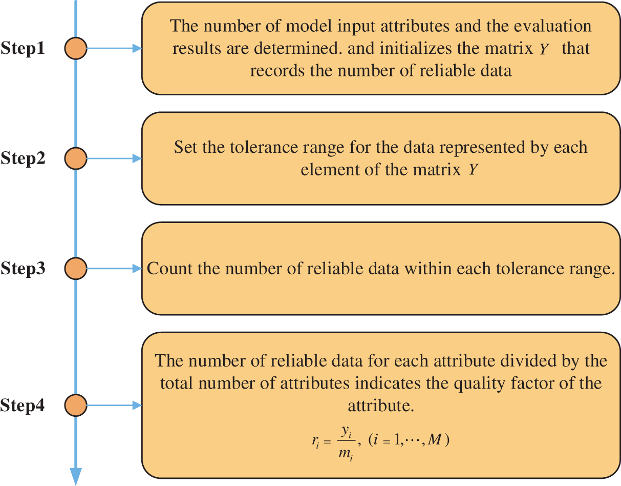
Figure 3: Calculation process of attribute quality factor

4.3 Rule Construction and Reasoning Process of BRB-SAQF

With the preparation of the above two subsections, the data features used as input attributes of the model are extracted, and the quality factor of each attribute is calculated. The next task is to use these data to construct the rules of the BRB-SAQF model. The basic structure of the kth rule Rk is described by Eq. (13).

Rk:if x1 is A1,x2 is A2,…,xM is AM Then y is {(D1,β1),…,(DN,βN)}∑n=1Nβn≤1With rule weight θk,attribute weight δ1,δ2,…,δMand attribute quality factor r1,r2,…,rM(13)

where x1,x2,…,xM denotes M input attributes of the model and A1,A2,…,AM denotes reference values of M attributes; y is a set of belief distributions described as {(D1,β1),…,(DN,βN)}, where D1,D2,…,DN are N levels defined by the model and β1,β2,…,βN represents the belief degree of each level. θk denotes the rule weight, δ1,δ2,…,δM represents the M attribute weight, and r1,r2,…,rM represents the M attribute quality factor. Among these parameters of the BRB-SAQF model, rule weight θk, attribute weight δ1,δ2,…,δM and belief degree β1,β2,…,βN are initialized by expert empirical knowledge.

When the rules of the model are constructed, the next problem to consider is incorporating the attribute quality factor into the reasoning process of BRB. In this paper, the reasoning process of the BRB model considering the quality factor of attributes can be expressed in the following six steps.

Step 1: The attribute matching degree is calculated. When the attribute data are input to the diagnosis model, the first step is to calculate the matching degree of corresponding reference points based on the input values and the reference values of attributes. The calculation process is described by Eq. (14).

αij={Aik+1−xiAik+1−Aik,j=kxi−AikAik+1−Aik,j=k+10,j=1,…,K,j≠k,j≠k+1(14)

where αij denotes the matching degree of the ith attribute in the jth reference value, xi is the current input attribute value, and Aik denotes the kth reference value of the ith attribute. When the Aik≤xi≤Aik+1 condition is satisfied, the above formula can calculate the matching degree of the attribute reference value.

Step 2: The fusion factor considering the attribute quality factor is calculated. In this step, the attribute quality factor and attribute weight are simultaneously considered and fused into one factor, which is calculated by Eqs. (15) and (16).

ci=δ¯i1+δ¯i−ri(15)

δ¯i=δimax{δi}(16)

where ri and δi are the attribute quality factor and attribute weight, respectively. The symbol δ¯i denotes the relative attribute weight. Eq. (15) shows that when the attribute quality factor is equal to 1, then ci is equal to 1.

Step 3: The matching degree of the kth rule is calculated. After calculating the attribute matching degree and fusion factor, the matching degree of the rules in the BRB must be calculated. When the matching degree of the rules is not equal to zero, this rule is activated; otherwise, this rule is not activated. The formula for calculating the rule-matching degree is shown in Eq. (17).

αk=∏i=1M(αki)ci(17)

where M is the number of attributes in the kth rule and αki denotes the ith attribute matching degree in the kth rule. The symbol ci is the fusion factor calculated in Step 2.

Step 4: After the rule matching degree is calculated and activated rules are determined, the activation weights of the rules must be calculated. The calculation method of the activation weights is shown in Eq. (18).

ωk=θkαk∑i=1Lθiαi,k=1,…,L(18)

where θk denotes the rule weight of rule k and αk denotes the rule matching degree. The letter L denotes the number of rules. If the rule is an activated, its activation weight is not equal to 0; otherwise, the activation weight is equal to 0. Note that 0≤ωk≤1, and ∑k=1Lωk=1.

Step 5: Multiple activated rules are fused, and the fused belief degree can be obtained. After those rules are determined to be activated, they are fused by an evidence reasoning (ER) parsing algorithm [27]. The calculation method is shown in Eqs. (19) and (20).

βn=μ[∏k=1L(ωkβn,k+1−ωk∑j=1Nβj,k)−∏k=1L(1−ωk∑j=1Nβj,k)]1−μ[∏k=1L(1−ωk)](19)

μ=[∑n=1N∏k=1L(ωkβn,k+1−ωk∑j=1Nβj,k)−(N−1)∏k=1N(1−ωk∑j=1Nβj,k)]−1(20)

where N denotes the fault diagnosis model identification framework with N diagnostic levels and L denotes the number of rules that have been activated. The symbol ωk denotes the activation weight of the rule and βj,k denotes the belief degree of consequence j in the rule k. The initial belief degree is determined by expert knowledge. By calculating Eqs. (19) and (20), the following result shown in Eq. (21) can be obtained.

S(x∗)={(D1,β1),…,(DN,βN)}(21)

where x∗ represents multiple attributes input into the model, including x1,x2,…,xM these M attributes. The symbols D1,D2,…,DN represent the identification framework levels of the model. β1,β2,…,βN represents the belief degree of each level.

Step 6: The final utility of the model is derived from the results of the fused belief degree. Assume that the utility of the nth level is described by u(Dn). The utility of S(x∗) is obtained by Eq. (22).

u(S(x∗))=∑n=1Nu(Dn)βn(22)

Through the above analysis, the inference process of BRB-SAQF is introduced. The whole inference process can be represented as shown in Fig. 4.

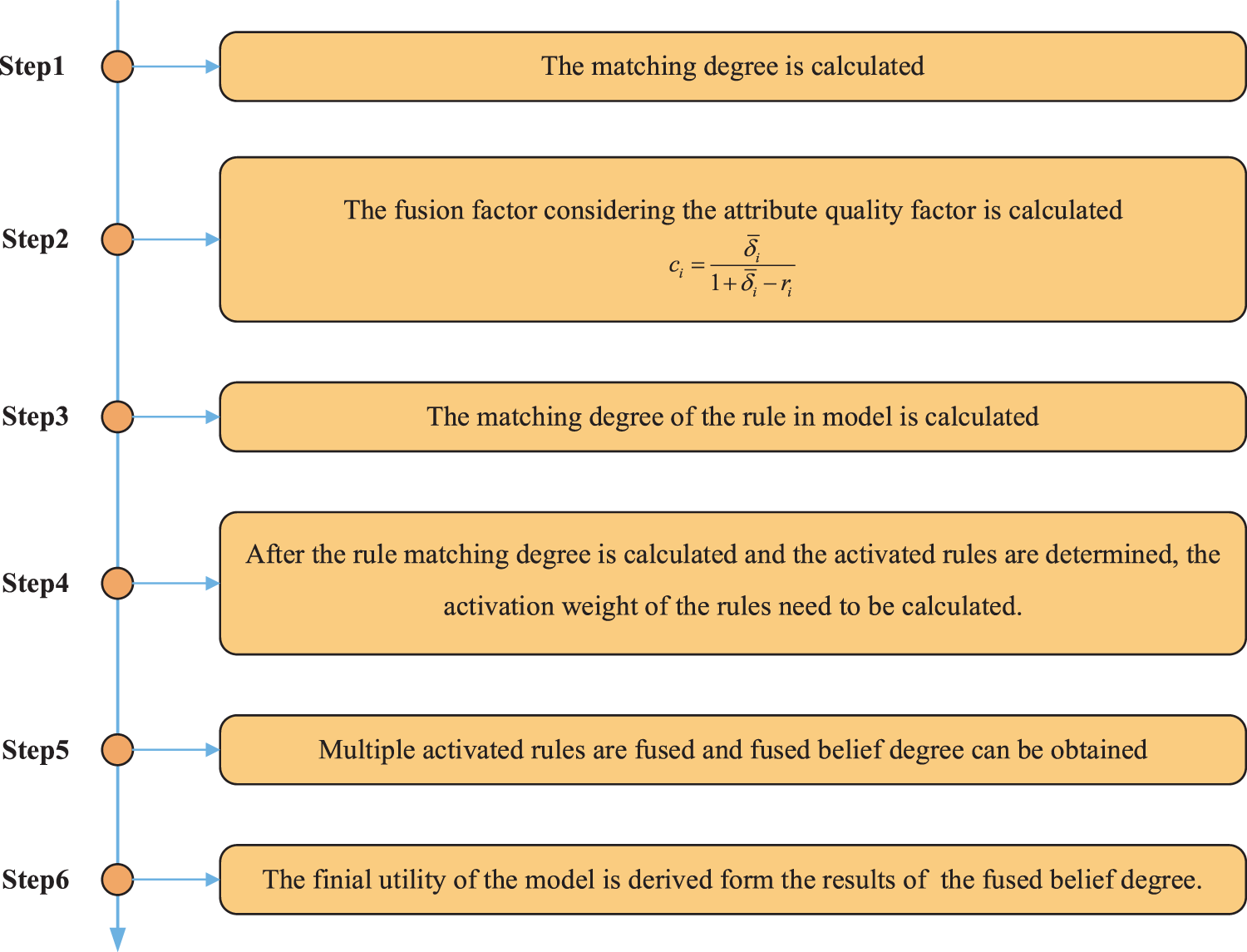
Figure 4: Reasoning process of BRB-SAQF

4.4 The Model Optimization Process

In Section 4.3, the initial values of rule weights, attribute weights, and belief degree of BRB-SAQF are determined by expert knowledge. However, when the model has many parameters and the expert has insufficient experience and knowledge, the initial setting of the parameters is not reasonable, which may affect the accuracy of the model diagnosis. Therefore, this paper proposes an optimization process of the model to improve the diagnostic accuracy of the model using a projection covariance matrix adaptation evolution strategy (P-CMA-ES) to optimize the parameters of the model [28,29]. The model’s parameters that need to be optimized need to satisfy the following conditions.

For rule weight θk, the conditions shown in Eq. (23) need to be satisfied.

0≤θk≤1,k=1,2,…,L(23)

For attribute weight δi, the conditions shown in Eq. (24) need to be satisfied.

0≤δi≤1,i=1,2,…,M(24)

For the belief degree of the corresponding consequent in each rule, the conditions shown in Eqs. (25) and (26) need to be satisfied.

0≤βn,k≤1,n=1,2,…,N,k=1,2,…,L(25)

∑n=1Nβn,k≤1,k=1,2,…,L(26)

After the parameters that need to be optimized and the constraints are determined, a metric to reflect the effectiveness of the optimization must be defined. Suppose the diagnosis result of the optimization process is resultoptimization, and the original result of the training data is resultorigin; then, the mean square error (MSE) between the two results is used to reflect the effect of parameter optimization. The MSE is calculated by Eq. (27).

MSE(η)=1T∑t=1T(resultoptimization−resultorigin)2(27)

where T denotes the number of data used to train the model parameters. The symbol η denotes the set of optimized parameters. Through the above analysis, the optimization process of the model can be understood as finding the minimum value of the MSE.

4.5 Model Building Process

By analyzing the contents of this section, the process of building a node fault diagnosis model for WSN based on BRB-SAQF can be divided into the following steps.

Step 1: The data features of the WSN node are extracted from the observed data and used as input attributes of the BRB-SAQF model.

Step 2: The quality factor of the model input attributes is calculated using the self-adaptive attribute quality factor calculation method.

Step 3: The model parameters are initialized, and the model rules are fused using the ER parsing algorithm.

Step 4: The initial parameters are optimized by P-CMA-ES to improve the diagnostic accuracy of the model.

5  Case Study

In this section, we conduct a case study based on sensor data from the Intel Berkeley Research Lab and compare BRB-SAQF with other fault diagnosis methods, including BRB-Sr, artificial neural networks, Gaussian regression, support vector machines, decision trees, and boosting trees. The case study is used to verify that the fault diagnosis method based on BRB-SAQF for the WSN nodes can effectively reduce the impact of noise data on the fault diagnosis process of the WSN nodes.

5.1 Fault Diagnosis Using BRB-SAQF

Step 1: The data in the dataset are preprocessed, and the set of diagnostic results for the model is defined. The dataset consists of temperature, humidity, light and voltage collected by 54 sensors. These sensors are distributed in a laboratory. Then, based on the distribution of the sensors and the trend of the data, the temperature data from sensors 1 to 4 from March 1st to 7th were selected for the study [30]. The dataset was preprocessed because the data were missing at some point. Meanwhile, Gaussian noise was added to the dataset simulation to verify that the model can effectively reduce the interference of noisy data [31,32]. The processed dataset has a total of 2,016 pieces of data with five minutes between two adjacent pieces of data, where the data of sensors 1 to 4 are shown in Fig. 5.

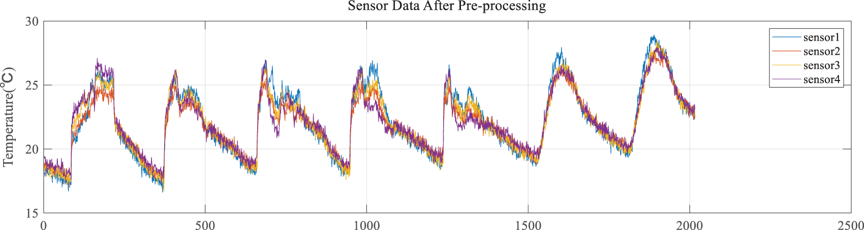
Figure 5: Sensor data after preprocessing

This paper uses offset faults, high-noise faults, outlier faults and fixed value faults as the types of sensor faults to be detected [33]. Next, based on the characteristics of the fault, the four types of faults mentioned above are simulated on sensor 1 using a software approach. The methods of fault data simulation are shown in Table 1, and the fault data after simulation are shown in Fig. 6.

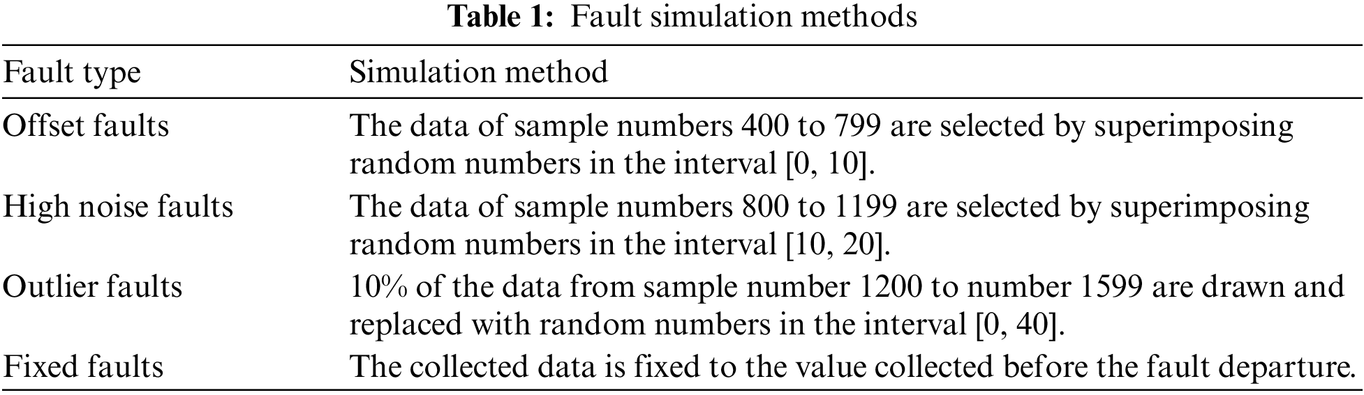
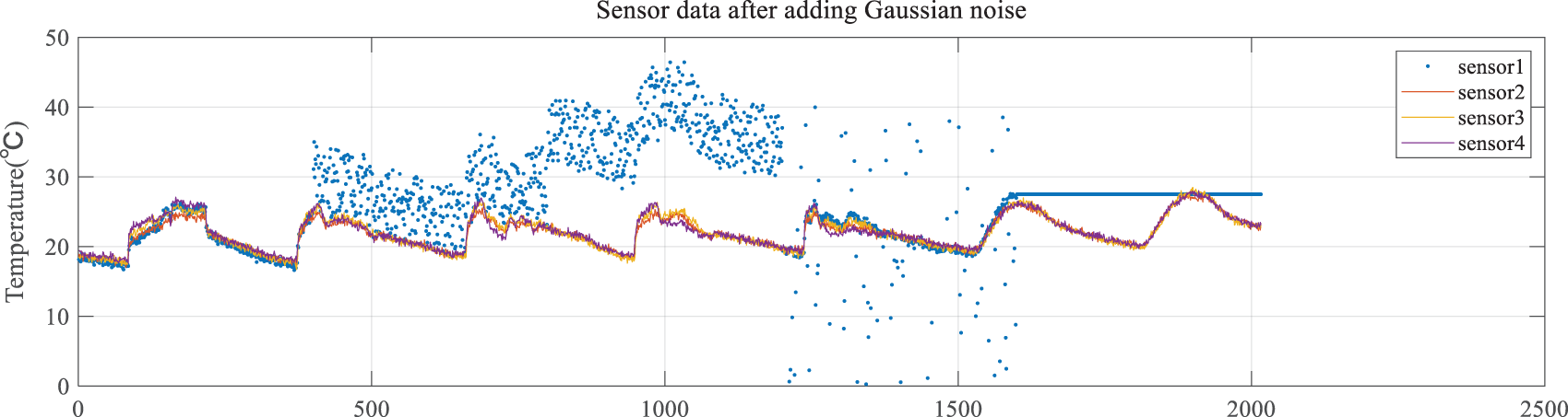
Figure 6: Sensor data after adding Gaussian noise

With the above introduction of the case study dataset, the output of the fault diagnosis model identification framework includes normal states (NS), offset faults (OSF), high-noise faults (HNF), outlier faults (OLF) and fixed value faults (FVF), which can be described by Eq. (28), and the corresponding reference values are shown in Eq. (29).

{NS,OSF,HNF,OLF,FVF}(28)

{0,1,2,3,4}(29)

Step 2: Sensor data features are extracted. After the data are prepared, the data features, including the mean gap and kurtosis, are extracted using the method introduced in Section 4.1 and as input attributes of the model. The time window for extracting data features is set to 12, and the extracted data features are normalized. The data features are shown in Figs. 7 and 8. The highlighted part in the figures displays unreliable data.

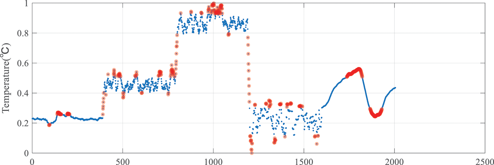
Figure 7: Mean gap data feature image

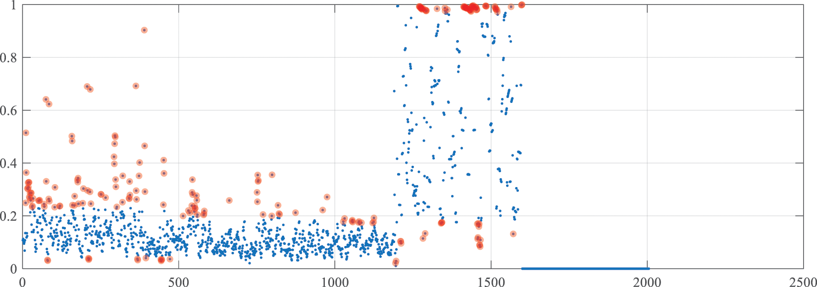
Figure 8: Kurtosis data feature image

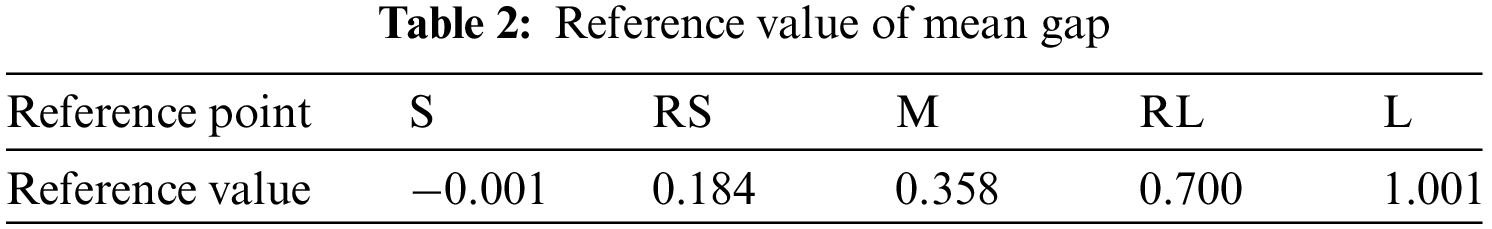
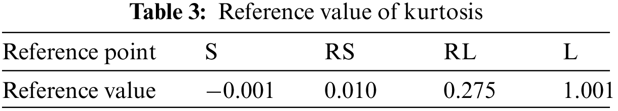
Step 3: The reference points and values for the model input attributes are determined. After the data features as input attributes of the model are extracted, each attribute’s reference values and points must be determined. The reference values and points for the mean gap and kurtosis are determined based on the data distribution characteristics in Figs. 7 and 8. The reference points of the mean gap are small (S), relatively small (RS), medium (M), relatively large (RL) and large (L). The reference values of the mean gap are shown in Table 2. The reference points of kurtosis are small (S), relatively small (RS), relatively large (RL) and large (L). The reference values of kurtosis are shown in Table 3.

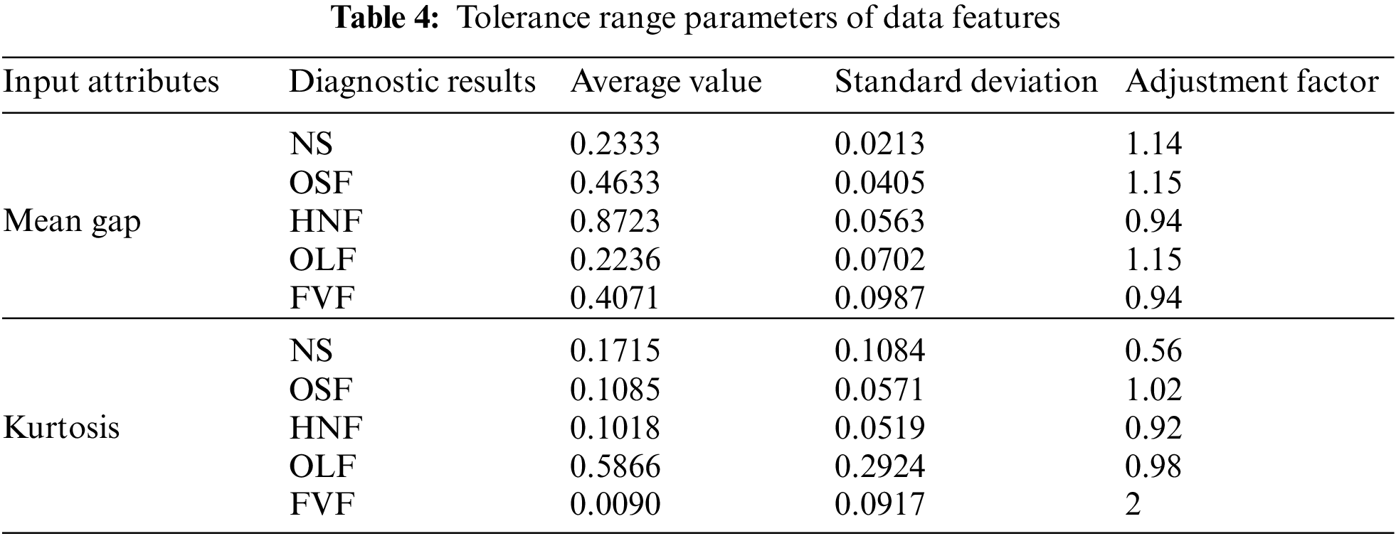
Step 4: The quality factors of each input attribute are calculated. In this step, the mean gap and kurtosis quality factors are calculated using the method described in Section 4.2. The setting of the tolerance ranges for different cases is shown in Table 4. The quality factors of the mean gap and kurtosis are calculated to be 0.7062 and 0.7276, respectively.

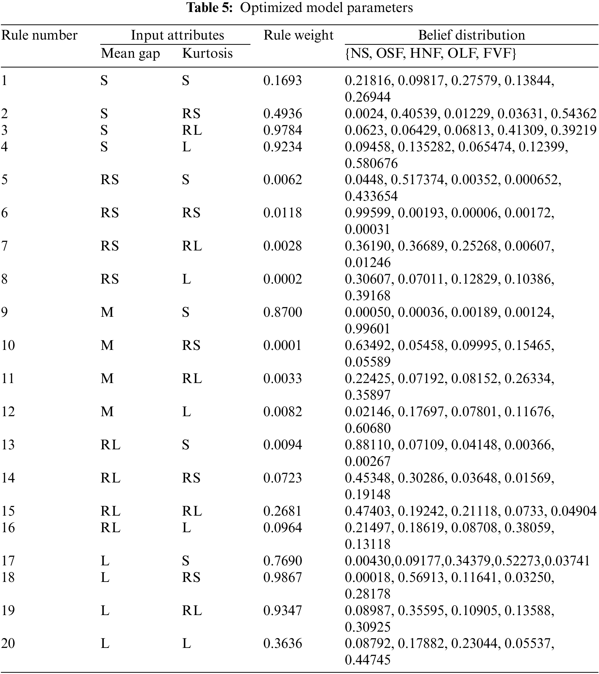
Step 5: The other parameters of the model are initialized. These parameters are optimized using the P-CMA-ES method proposed in Section 4.4. After optimization, the parameters are shown in Table 5, where each row represents a rule in the model. Finally, the model inference process presented in Section 4.3 is used together with the optimized parameters to diagnose sensor faults and produce results.

Step 6: The evaluation indices of the fault diagnosis model are determined. The overall accuracy, false-negative rate (FNR) and false-positive rate (FPR) are used as evaluation indices to verify the method’s validity. It is assumed that samples without faults are negative samples and the samples with faults are positive samples. The formulas for the above indices are shown in Eqs. (30)–(32).

Accuracy=NumrightNumsample(30)

where Numright represents the number of samples correctly diagnosed by the model. The expression Numsample denotes the total number of samples.

FNR=FNTP+FN(31)

where FN denotes the number of samples with false negatives and TP denotes the number of samples with true positives.

FPR=FPFP+TN(32)

where FP represents the number of samples with false positives and TN represents the number of samples with true negatives.

5.2 Comparison with Other Methods

It is compared with other methods to verify the effectiveness of the proposed method proposed in this paper and the improvement of the BRB-Sr method. These include BRB-Sr, artificial neural networks, Gaussian regression processes, support vector machines, decision trees and boosting trees. The fault diagnosis results compared with the BRB-Sr method are shown in Fig. 9, and the evaluation indices of the different methods are shown in Figs. 10–12.

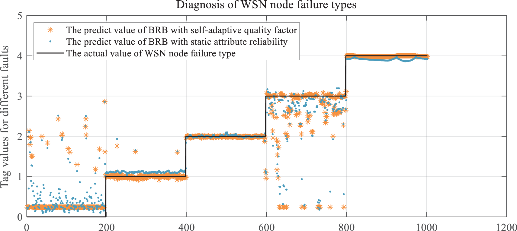
Figure 9: Comparison of diagnostic results of BRB-SAQF and BRB-Sr

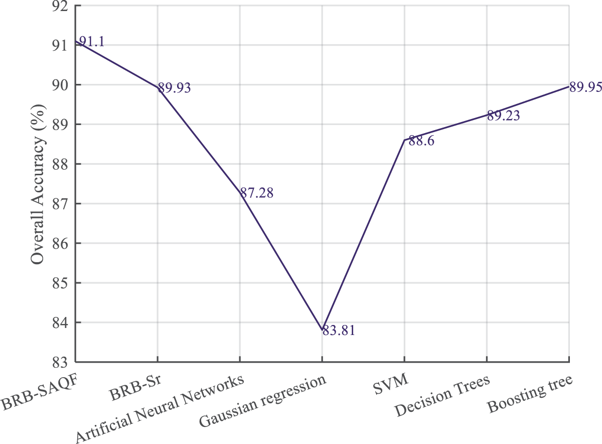
Figure 10: Overall accuracy of different methods

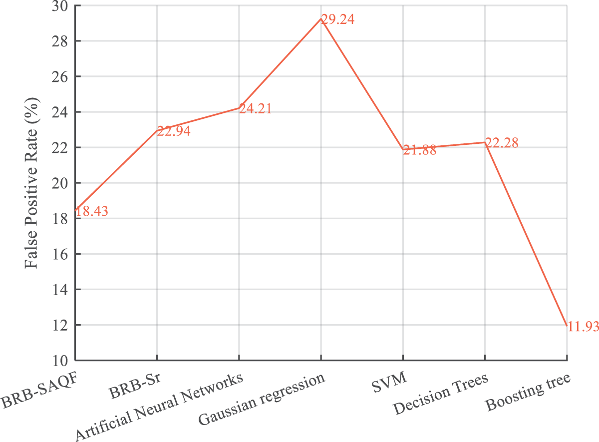
Figure 11: False positive rate of different methods

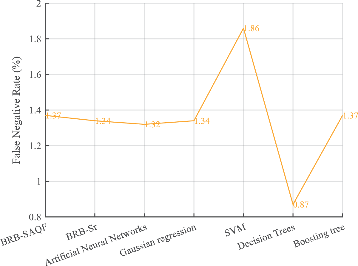
Figure 12: False negative rate of different methods

By comparing the diagnostic results of BRB-SAQF and BRB-Sr, it is evident that the value of BRB-SAQF is closer to the actual situation, especially in the reference value of 0. After testing, the overall accuracy, FNR, and FPR of BRB-SAQF are 91.1%, 18.43%, and 1.37%. The BRB-Sr values are 89.93%, 22.94%, and 1.34%, respectively. The reason for the scattering diagnostic results of method BRB-Sr is that the tolerance range of method BRB-Sr cannot wholly count the unreliable data, which leads to the inaccurate calculation of the attribute reliability. The quality factor calculation method obtained by improving the static attribute reliability calculation method can effectively count the unreliable data in the middle region of the fluctuating attribute data, enabling a more focused diagnosis.

By comparing the evaluation indices of different methods. First, it can be concluded that the results of the BRB-SAQF and BRB-Sr methods are higher than those of the other methods in terms of overall accuracy. Second, regarding the false-positive rate, the BRB-SAQF method has a relatively low false-positive rate, making it less likely to misdiagnose nodes as faults. Finally, in terms of the false negative rate, the difference between all the above methods is slight, fluctuating at approximately 1.3%, and there is no substantial gap between the methods. The reasons for the above results can be summarized in the following points. First, the BRB-SAQF introduces a quality factor and improves the calculation method of attribute reliability, which can count unreliable data more effectively. The attribute quality factor calculation is more accurate. Second, the inference process of BRB-SAQF is essentially similar to BRB’s, which can handle uncertain information, including ambiguity, randomness and ignorance [15]. Finally, the BRB-SAQF model parameter settings come from expert experience and knowledge, and the parameter settings are more reasonable. Compared with the neural network approach, the BRB-SAQF method is more interpretable and more applicable to training with small, unbalanced samples. With the combined effect of the above factors, the BRB-SAQF method improves the fault diagnosis accuracy of the WSN node.

6  Conclusion

The following conclusions can be obtained through the analysis of related work and the examination of case studies. Some shortcomings exist in the commonly used fault diagnosis methods for WSN nodes. First, the methods do not consider the influence of environmental noise collected by the sensors during the fault diagnosis process. Second, with the weight and bias parameters in the method, the neural network-based methods aim to fit a nonlinear function and require many uniform fault samples to train model parameters. Finally, the attribute reliability calculation renders the BRB-Sr approach unable to count the unreliable data in the middle segment when the attribute value changes considerably, which affects the fault diagnosis accuracy and needs to be optimized to obtain a more accurate diagnostic result.

The BRB-SAQF model is proposed as a fault diagnosis method to solve the above shortcomings. First, the calculation method of the attribute quality factor is designed to compensate for the shortcomings of the static attribute reliability calculation method to improve the accuracy of fault diagnosis. Second, the parameters in the BRB-SAQF method represent the rules, weights and quality factors of the attributes and the probability of possible failures. Experts initialize these parameters based on their experience and knowledge, which are more reasonable and interpretable. Finally, because the BRB method has the advantage of small sample training, the number of fault samples must be smaller. Through the case study in Section 5 of this article, the accuracy of the method proposed in this paper is improved compared with that of the BRB-Sr and other methods, and the distribution of the predicted values is more focused, which proves the effectiveness of the method proposed in this paper.

However, BRB-SAQF, as a derived method of BRB, has the following disadvantages. First, when the method has more premise attributes or reference points for the attributes, BRB-SAQF causes the problem of rule combination explosion, i.e., the number of rules is huge. As a result, initializing the parameters is more complicated. Therefore, in our future research, we will focus on the following aspects:

1)   Research and design methods to reduce the number of rules to solve the problem of rule combination explosion.

2)   Design the belief rule base for the network structure so that the number of rules per submodule can be reduced while reducing the difficulty of initializing the parameters.

3)   Research and design the construction method of a network structure BRB so that the structure of the model can be more consistent with the working mechanism of the diagnosed object.

Funding Statement: This work was partly supported by the Postdoctoral Science Foundation of China under Grant No. 2020M683736, partly by the Teaching reform project of higher education in Heilongjiang Province under Grant No. SJGY20210456, partly by the Natural Science Foundation of Heilongjiang Province of China under Grant No. LH2021F038, partly by the Haiyan foundation of Harbin Medical University Cancer Hospital under Grant No. JJMS2021-28, and partly by the graduate academic innovation project of Harbin Normal University under Grant Nos. HSDSSCX2022-17, HSDSSCX2022-18 and HSDSSCX2022-19. The recipient of all the above funds is W. He.

Conflicts of Interest: The authors declare that they have no conflicts of interest to report regarding the present study.

References

1. M. Angurala and V. Khullar, “A survey on various congestion control techniques in wireless sensor networks,” International Journal on Recent and Innovation Trends in Computing and Communication, vol. 10, no. 8, pp. 47–54, 2022. [Google Scholar]
2. P. Patil, Waghole, Deshpande and Karykarte, “Sectoring method for improving various QoS parameters of wireless sensor networks to improve lifespan of the network,” International Journal on Recent and Innovation Trends in Computing and Communication, vol. 10, no. 6, pp. 37–43, 2022. [Google Scholar]
3. M. S. Rajan, G. Dilip, N. Kannan, M. Namratha, S. Majji et al., “Diagnosis of fault node in wireless sensor networks using adaptive neuro-fuzzy inference system,” Applied Nanoscience, 2021. https://doi.org/10.1007/s13204-021-01934-0. [Google Scholar]
4. M. Zhao, Z. Tian and T. W. S. Chow, “Fault diagnosis on wireless sensor network using the neighborhood kernel density estimation,” Neural Computing and Applications, vol. 31, no. 8, pp. 4019–4030, 2019. [Google Scholar]
5. U. Saeed, S. U. Jan, Y. D. Lee and I. Koo, “Fault diagnosis based on extremely randomized trees in wireless sensor networks,” Reliability Engineering & System Safety, 2021. https://doi.org/10.1016/j.ress.2020.107284. [Google Scholar]
6. Z. Noshad, N. Javaid, T. Saba, Z. Wadud, M. Q. Saleem et al., “Fault detection in wireless sensor networks through the random forest classifier,” Sensors, vol. 19, no. 7, pp. 1568, 2019. [Google Scholar]
7. E. Moridi, M. Haghparast and M. Hosseinzadeh, “Novel fault management framework using markov chain in wireless sensor networks: FMMC,” Wireless Personal Communications, vol. 114, no. 1, pp. 583–608, 2020. [Google Scholar]
8. R. R. Swain, M. K. Pabitra and D. Tirtharaj, “Multifault diagnosis in WSN using a hybrid metaheuristic trained neural network,” Digital Communications and Networks, vol. 6, no. 1, pp. 86–100, 2018. [Google Scholar]
9. M. M. Gharamaleki and B. Shahram, “A new distributed fault detection method for wireless sensor networks,” IEEE Systems Journal, vol. 14, no. 4, pp. 4883–4890, 2020. [Google Scholar]
10. S. Mohapatra, P. M. Khilar and R. R. Swain, “Fault diagnosis in wireless sensor network using clonal selection principle and probabilistic neural network approach,” International Journal of Communication Systems, vol. 32, no. 16, 2019. https://doi.org/10.1002/dac.4138. [Google Scholar]
11. R. Regin, S. S. Rajest and B. Singh, “Fault detection in wireless sensor network based on deep learning algorithms,” EAI Transactions on Scalable Information Systems, 2021. https://eudl.eu/doi/10.4108/eai.3-5-2021.169578. [Google Scholar]
12. R. R. Swain, P. M. Khilar and T. Dash, “Neural network based automated detection of link failures in wireless sensor networks and extension to a study on the detection of disjoint nodes,” Journal of Ambient Intelligence and Humanized Computing, vol. 10, no. 2, pp. 593–610, 2018. [Google Scholar]
13. A. Javaid, N. Javaid, Z. Wadud, T. Sava, O. E. Sheta et al., “Machine learning algorithms and fault detection for improved belief function based decision fusion in wireless sensor networks,” Sensors, vol. 19, no. 6, pp. 1334, 2019. [Google Scholar]
14. J. B. Yang, J. Liu, J. Wang, H. S. Sii and H. W. Wang, “Belief rule-base inference methodology using the evidential reasoning approach-RIMER,” IEEE Transactions on Systems, Man, and Cybernetics-Part A: Systems and Humans, vol. 36, no. 2, pp. 266–285, 2006. [Google Scholar]
15. Z. Zhou, Y. Cao, G. Hu, Y. Zhang, S. Tang et al., “New health-state assessment model based on belief rule base with interpretability,” Science China Information Sciences, vol. 64, no. 7, pp. 1–15, 2021. [Google Scholar]
16. Z. J. Zhou, G. Y. Hu, C. H. Hu, C. L. Wen and L. L. Chang, “A survey of belief rule-base expert system,” IEEE Transactions on Systems, Man, and Cybernetics: Systems, vol. 51, no. 8, pp. 4944–4958, 2019. [Google Scholar]
17. G. Wang, Y. Cui, J. Wang, L. Wu and G. Hu, “A novel method for detecting advanced persistent threat attack based on belief rule base,” Applied Sciences, vol. 11, no. 21, pp. 9899, 2021. [Google Scholar]
18. Z. Feng, Z. Zhou, C. Hu, X. Ban and G. Hu, “A safety assessment model based on belief rule base with new optimization method,” Reliability Engineering & System Safety, vol. 203, 2020. https://doi.org/10.1016/j.ress.2020.107055. [Google Scholar]
19. H. L. Zhu, S. S. Liu, Y. Y. Qu, X. X. Han, W. He et al., “A new risk assessment method based on belief rule base and fault tree analysis,” Proceedings of the Institution of Mechanical Engineers, Part O: Journal of Risk and Reliability, vol. 236, no. 3, pp. 420–438, 2021. [Google Scholar]
20. Y. Cao, Z. J. Zhou, C. H. Hu, S. W. Tang and J. Wang, “A new approximate belief rule base expert system for complex system modelling,” Decision Support Systems, vol. 150, 2021. https://doi.org/10.1016/j.dss.2021.113558. [Google Scholar]
21. W. He, P. L. Qiao, Z. J. Zhou, G. Y. Hu, Z. C. Feng et al., “A new belief-rule-based method for fault diagnosis of wireless sensor network,” IEEE Access, vol. 6, pp. 9404–9419, 2018. [Google Scholar]
22. Z. Feng, Z. J. Zhou, C. Hu, L. L. Chang, G. Y. Hu et al., “A new belief rule base model with attribute reliability,” IEEE Transactions on Fuzzy Systems, vol. 27, no. 5, pp. 903–916, 2018. [Google Scholar]
23. D. N. Joanes and C. A. Gill, “Comparing measures of sample skewness and kurtosis,” Journal of the Royal Statistical Society (Series DThe Statistician, vol. 47, no. 1, pp. 183–189, 1998. [Google Scholar]
24. W. He, L. C. Liu and J. P. Yang, “Reliability analysis of stiffened tank-roof stability with multiple random variables using minimum distance and lagrange methods,” Engineering Failure Analysis, vol. 32, pp. 304–311, 2013. [Google Scholar]
25. B. K. Lad and M. S. Kulkarni, “A parameter estimation method for machine tool reliability analysis using expert judgement,” International Journal of Data Analysis Techniques and Strategies, vol. 2, no. 2, pp. 155–169, 2010. [Google Scholar]
26. X. B. Xu, J. Zheng, D. L. Xu and J. B. Yang, “Information fusion method for fault diagnosis based on evidential reasoning rule,” Journal of Control Theory and Applications, vol. 32, pp. 1170–1182, 2015. [Google Scholar]
27. Z. J. Zhou, C. H. Hu, G. Y. Hu, X. X. Han, B. C. Zhang et al., “Hidden behavior prediction of complex systems under testing influence based on semiquantitative information and belief rule base,” IEEE Transactions on Fuzzy Systems, vol. 23, no. 6, pp. 2371–2386, 2015. [Google Scholar]
28. Z. Feng, W. He, Z. Zhou, X. Ban, C. Hu et al., “A new safety assessment method based on belief rule base with attribute reliability,” IEEE/CAA Journal of Automatica Sinica, vol. 8, no. 11, pp. 1774–1785, 2020. [Google Scholar]
29. X. Cheng, S. Liu, W. He, P. Zhang, B. Xu et al., “A model for flywheel fault diagnosis based on fuzzy fault tree analysis and belief rule base,” Machines, vol. 10, no. 2, pp. 73, 2022. [Google Scholar]
30. H. Zhu, W. Geng and J. Hanm, “Constructing a WSN node fault detection model using the belief rule base,” CAAI Transactions on Intelligent Systems, vol. 16, no. 3, pp. 511–517, 2021. [Google Scholar]
31. H. Zhu, J. Li, Y. Gao and G. Cheng, “Consensus analysis of UAV swarm cooperative situation awareness,” in Proc. ICVRIS, Zhangjiajie, Hunan, China, pp. 415–418, 2020. [Google Scholar]
32. Y. C. Ho, “On the perturbation analysis of discrete-event dynamic systems,” Journal of Optimization, Theory and Applications, vol. 46, no. 4, pp. 535–545, 1985. [Google Scholar]
33. N. Ramanathan, E. Kohler and D. Estrin, “Towards a debugging system for sensor networks,” International Journal of Network Management, vol. 15, no. 4, pp. 223–234, 2005. [Google Scholar]
Cite This Article
Copyright © 2023 The Author(s). Published by Tech Science Press.
This work is licensed under a Creative Commons Attribution 4.0 International License , which permits unrestricted use, distribution, and reproduction in any medium, provided the original work is properly cited.
Downloads
Citation Tools