Deepfake Video Detection Based on Improved CapsNet and Temporal–Spatial Features

1  Introduction

In recent years, the optimization of deep neural networks and the improved performance of the graphics processing unit (GPU) led to the rapid development of deepfake technology, allowing the automatic creation of more realistic forged videos. Using deepfake technology, one can superimpose the facial image of the target person onto the corresponding position of the face of the original person in the video, thus creating a video of the target person making statements or performing actions that did not actually take place, in order to confuse viewers [1].

Deepfake videos have spread rapidly with the help of online platforms, posing risks to individuals, societies, and countries. In June 2019, DeepNude software used the deepfake technology to generate nude pictures of female victims, violating the privacy and reputation of more than 104,000 women. Telecommunication fraud, performed through forged videos and multiple rounds of dialogues, has likewise become a trend [2]. Social engineering takes advantage of the victims’ psychological weaknesses to carry out the deception. If combined with deepfake technology, social engineering may achieve a better deception effect [3]. For example, in August 2019, criminals created a voice model of a German energy company’s president and successfully defrauded the company’s UK branch, stealing EUR 220,000. During the U.S. election in April 2020, former U.S. President Donald Trump retweeted a video made by deepfake technology to vilify current President Joe Biden. Thus, politicians can use the technology to disrupt elections, manipulate public opinion and trigger a crisis of confidence [4,5]. Therefore, the timely detection of deepfake videos is among the key tasks in cyberspace security.

Mainstream deepfake video detection methods are divided into two categories: one based on video intraframe feature differences that learns the spatial features of a single frame and makes a comprehensive decision based on the prediction results of each frame, and the other based on video interframe feature differences, which treats deepfake videos as time-series data, uses the time-series algorithm to capture the differences of the temporal features between real and fake videos frame-by-frame, and then classifies them.

In this study, we propose iCapsNet–TSF, a deepfake video detection method based on improved CapsNet and the fusion of temporal–spatial features. The iCapsNet–TSF method combines the capsule network and optical flow algorithm to detect deepfake videos for the first time. Compared with previous related studies, our method makes comprehensive decisions based on the temporal and spatial features of facial images, which significantly improves the detection accuracy.

The organization of our paper is as follows. Section 1 introduces the basic concepts and relevant background of deepfake technology. Section 2 introduces the studies related to the deepfake video detection method. Section 3 introduces the detection method proposed in this study. Section 4 presents the experiments used to evaluate the effectiveness of the proposed method through a variety of indexes. Section 5 lists the conclusions, summarizing the work conducted in this study and considering future directions of this field.

2  Related Work

Deepfake video detection methods based on feature extraction can be divided into detection based on video intra- and interframe features. The procedures for both are as follows: (1) a key frame extraction and face detection algorithm are used to convert video data into facial image data, and then (2) a deep neural network is used to extract the spatial or temporal feature vector of the facial image, and, finally, (3) a classification function is used to distinguish between real and fake faces.

The detection method based on the feature extraction uses the deep learning technology, which involves the learning of massive datasets and the use of a back-propagation algorithm to identify the optimal detection model, significantly improving the detection by saving manpower and more accurately distinguishing falsified faces.

2.1 Detection Based on Video Intraframe Features

The detection method based on video intraframe features refers to the use of traditional algorithms, machine learning algorithms, or deep learning models to learn the spatial features of a single frame of a deepfake video and then making a comprehensive decision based on the prediction result of each frame. This method can fully extract spatial features, whereas it cannot fully use the temporal features of deepfake videos, because it ignores the fact that the videos themselves rely on temporal data. The essence of this method is the image detection, which can detect forged videos with high accuracy while minimizing parameter redundancy.

In addition to other data, traditional algorithms consider the attributes of the video, such as the frame rate and brightness. Koopman et al. [6] calculated normalized cross-correlation scores to distinguish the deepfake videos based on the differences in the light perception noise during the camera shooting. Luo et al. [7] found that the high-frequency signal of the image removed the color texture, which helps to more effectively distinguish real and fake videos. Therefore, high-frequency signal features were fused with original RGB features by the attention mechanism, and the videos were finally classified.

Machine learning algorithms are often used to classify falsified faces by extracting a one-dimensional vector that represents facial features. On the basis of large differences in the colors of eyes, shadows appearing on the edges of the nose, and littery geometric rules of teeth on falsified faces, Matern et al. [8] extracted facial feature vectors via computer vision methods, such as color histograms and color aggregation vectors, and then used the k-nearest neighbor (KNN) algorithm to classify them. Yang et al. [9] found that head poses of the original face change during face tampering, and the authors used the differences between the feature vectors of the tampered parts and the whole face as a criterion to obtain a classification with the help of the support vector machine (SVM) algorithm. Durall et al. [10] extracted the two-dimensional power spectrum of video frames via the discrete Fourier transform, which is compressed into a one-dimensional feature vector using orientation averaging, and then classified using a logistic regression algorithm.

When detecting deepfake videos, traditional machine learning algorithms must often extract facial features manually. Furthermore, because of classifier limitations, it is difficult to extract deep pixel-level spatial features of the image.

Therefore, generative networks and convolutional neural networks (CNNs) are gradually used to detect deepfake videos. Cozzolino et al. [11] proposed a novel approach that learns temporal facial features by means of metric learning coupled with an adversarial training strategy. Using a three-dimensional morphable model (3DMM), the authors processed videos of different identities on a frame-by-frame basis and trained the Temporal ID Network to embed the extracted features. To incentivize this network to focus on temporal aspects rather than visual cues, they jointly trained the 3DMM Generative Network to transform extracted features to fool its discriminative counterpart.

Afchar et al. [12] argued that the images’ low-layer noise features degrade with video compression, and high-layer semantic features are difficult to use as the basis for detection. Therefore, they proposed the mesoscopic network (MesoNet) combined with the Inception module to classify deepfake videos. Zhou et al. [13] proposed a two-stream CNN network employing RGB and noise convolution layers to extract pixel and noise features of video frames, and then fuse the two features to improve the detection accuracy. Nguyen et al. [14] used CapsNet to learn detailed information about the facial pose (position, hue, texture) and extract richer spatial features of the faces. Zhu et al. [15] proposed a combination of direct light and common texture to detect deepfake videos. At the same time, the supervised attention mechanism highlights the tampered areas to detect facial details. Wang et al. [16] proposed an attention-based data enhancement framework to guide detectors to refine and expand their attention. This method tracks and occludes the top-N sensitive areas of the faces and encourages the detectors to further explore previously ignored areas to obtain more accurate results.

With the development of the deep learning model, relevant studies presented at the top conferences in the last two years include the following. Li et al. [17] proposed the Frequency-aware Discriminative Features Learning (FDFL) framework, which uses a new single-center loss to reduce the intraclass changes in natural faces, so as to increase interclass differences in the embedded space. Simultaneously, they developed an adaptive frequency feature generation module, which mines subtle artifacts from the frequency domain in a data-driven manner. Zhao et al. [18] designed a Patch-wise Consistency Learning (PCL) branch to send the middle layer of the backbone network to different encoders and subsequently dot-multiply the results to provide additional supervision information for the backbone network and guide the model to pay attention to the similarity between forged and adjacent areas. Dong et al. [19] proposed an Identity Consistency Transformer (ICT), a novel facial video forgery detection method focusing on high-level semantics—specifically, identity information—and detecting a suspicious face by determining the identity inconsistency in inner and outer facial regions. The ICT incorporates a consistency loss to determine the identity consistency and exhibits superior generalization ability across different deepfake datasets.

Shao et al. [20] proposed the Seq-DeepFake Transformer (SeqFakeFormer) to detect forged images. First, they captured spatial manipulation traces of the image through self-attention modules in the transformer encoder, and then added the Spatially Enhanced Cross-Attention (SECA) module to generate different spatial weight maps for corresponding manipulations to carry out cross-attention. Wang et al. [21] proposed a novel Shuffled Style Assembly Network (SSAN) to extract and reassemble different contents and style features for a stylized feature space of facial images. Then, to obtain a generalized representation, a contrastive learning strategy was developed to emphasize liveness-related style information while suppressing domain-specific information. Gu et al. [22] proposed a Progressive Enhancement Learning Framework (PELF), which utilized both RGB information and fine-grained frequency information. Sun et al. [23] proposed Dual Contrastive Learning (DCL), which specially constructed positive and negative paired data and performed designed contrastive learning at different granularities to learn generalized feature representation. Specifically, they proposed Inter-Instance Contrastive Learning (Inter-ICL) based on the hard sample selection strategy to promote task-related discriminant feature learning.

2.2 Detection Based on Video Interframe Features

Because deepfake videos are synthesized frame-by-frame during the generation process, it is difficult to consider the previously forged frame sequence. People in the forged video will have a significantly lower frequency of blinking, and facial movements will be uncoordinated. Besides, the face brightness will change when the video is played frame-by-frame. Therefore, it can be captured by the algorithms considering temporal features.

The detection method based on video interframe features usually classifies deepfake videos according to the temporal features. However, it is sensitive to the length of frames, cannot effectively extract temporal features from the videos with short playback times, and lacks the learning of detailed spatial features of forged faces.

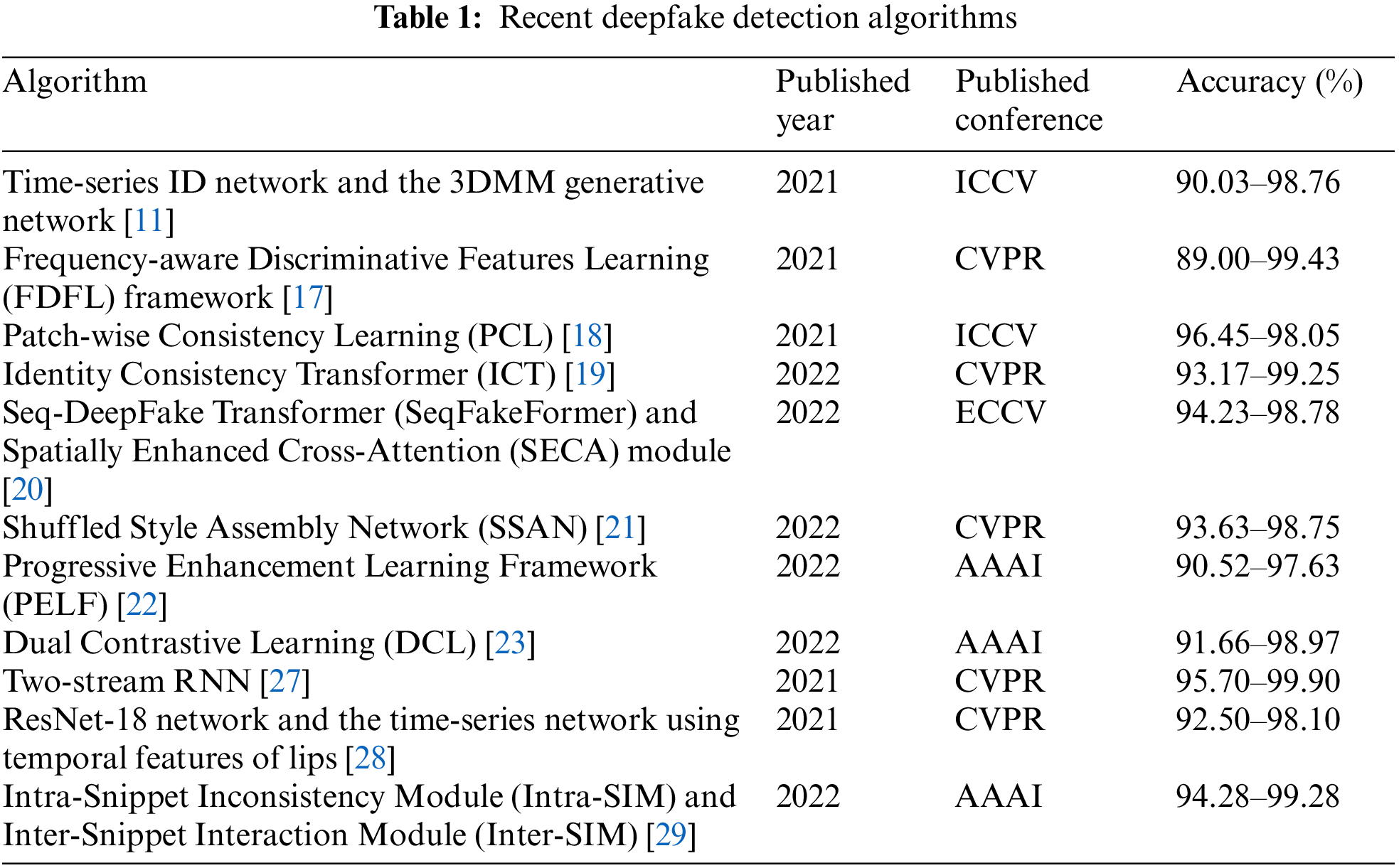
Sabir et al. [24] adopted the recurrent convolutional strategy. To detect deepfake videos, the CNN was used to extract the facial spatial features of each frame of the video, after which the recurrent neural network (RNN) was used to learn the time-series changes about facial features. Several studies found that the blinking frequencies of real and fake faces differ. Li et al. [25] used this observation for the identification, extracting the eye-distinguishing features of faces using the visual geometry group (VGG) network, and then used long short-term memory (LSTM) to learn the blinking frequency features of real and fake faces. Amerini et al. [26] used PWC-Net and LK algorithms to extract the optical flow vectors, and VGG16 was used to capture the difference between real and fake faces. For the preprocessing, Sun et al. [27] designed a calibration module to obtain a more accurate sequence of facial landmarks. They embedded the landmarks into two types of feature vectors, and then used the two-stream RNN to mine the time information and determine its authenticity. One feature vector serves to simulate the movement pattern of the facial shape, and the other is regarded as the velocity pattern used to capture the discontinuity of time. The high-level temporal semantic features of lips are difficult to forge by existing methods. Haliassos et al. [28] first pretrained the ResNet-18 network and the time-series network in the lip-reading task, fixed the ResNet-18 network, and trained only the time-series network so as to extract lip features that can help determine real and fake videos and realize the most advanced generalization of the forgery type. Gu et al. [29] studied the local motion information in videos and proposed a new video sampling unit, “Snippet”, which contains some local continuous video frames. Furthermore, the Intra-Snippet Inconsistency Module (Intra-SIM) and Inter-Snippet Interaction Module (Inter-SIM) were carefully designed to establish the inconsistent dynamic modeling framework. Specifically, Intra-SIM uses two-way time difference operations and learnable convolution kernels to mine the subtle motion in each “Snippet”. Inter-SIM is then used to facilitate the information interaction among “Snippets” to form a global representation. Table 1 shows the recent deepfake detection algorithms presented at the top conferences in the last two years.

3  Deepfake Video Detection Method

In this study, a deepfake video detection method, iCapsNet–TSF, is proposed, as shown in Fig. 1.

Figure 1: Deepfake video detection based on improved CapsNet and temporal–spatial features

The deepfake video detection method based on improved CapsNet and temporal–spatial features includes four stages: data processing, optical flow feature extraction, capsule network training, and classification of real and fake faces.

(1)   Data processing: Key frame extraction and face detection algorithms are used to transform video data into image data to form a spatial feature dataset. A sharpening operation is used to refine the image. Gaussian blur is added to reduce image noises. Data on the image are standardized and normalized to enhance the generalization ability of the model.

(2)   Optical flow feature extraction: Using the Lucas–Kanade (LK) optical flow algorithm, the best frame extraction strategy is selected to extract the temporal features of videos to form a dataset of temporal–spatial features. This dataset provides rich image features for the model, such that we can fully learn the temporal–spatial feature distribution of facial images.

(3)   Capsule network training: The VGG network is used to preliminarily extract facial features. The feature image is sent to the capsule network for training. During the training process, the dynamic routing algorithm (DRA) of the capsule network is improved in terms of the weight initialization and weight updating. Then, the improved dynamic routing algorithm (iDRA) and the corresponding improved CapsNet (iCapsNet) model are proposed.

(4)   Classification: After training the model on the temporal–spatial feature dataset, the cross-entropy loss function is used to evaluate the difference between predicted and true values. Then, the softmax function is used to obtain a binary classification of real and fake videos.

3.1 Optical Flow Feature Extraction

3.1.1 Optical Flow Algorithm

Optical flow is defined as the instantaneous velocity of the pixel motion in sequential images [30]. The optical flow algorithm analyzes the correlation between adjacent frames by estimating their optical flow. Therefore, the optical flow algorithm is often used to process video data.

There are two assumptions for calculating the optical flow between adjacent frames. Assumption (1): the brightness and color of the same pixel in two adjacent frames of the video remain stable. Assumption (2): the video is continuous, and the position of the target pixel does not change significantly within a short time.

Let the luminance of the pixel point (x,y) in the initial frame at moment t be I(x,y,t). The displacement at time δt is (δx,δy), such that the brightness in the adjacent frame is I(x+δx,y+δy,t+δt). The displacement of pixels in three dimensions can be identified intuitively, as shown in Fig. 2.

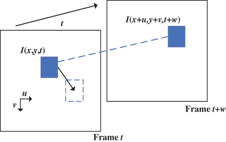
Figure 2: Visual presentation of pixel movement

According to Assumption (1), the brightness of the pixel remains constant during the motion of adjacent frames, as shown in Eq. (1).

I(x,y,t)=I(x+δx,y+δy,t+δt)(1)

Expanding the right-hand side of Eq. (1) using a first-order Taylor series yields Eq. (2):

I(x+δx,y+δy,t+δt)=I(x,y,t)+∂I(x,y,t)∂xδx+∂I(x,y,t)∂yδy+∂I(x,y,t)∂tδt+ε(2)

where ε represents a second-order and higher-order infinitesimal constant. As it is assumed that the pixel motion displacement is small, ε can be ignored. Dividing Eq. (2) by δt, we obtain Eq. (3).

∂I(x,y,t)∂xδxδt+∂I(x,y,t)∂yδyδt+∂I(x,y,t)∂t=0(3)

Let Vx=δxδt and Vy=δyδt denote the instantaneous velocity of the pixel moving along the x- and y-axis, respectively. Let Ix=∂I∂x, Iy=∂I∂y, and It=∂I∂t denote the difference in the brightness of the pixel along the x-, y-, and t-axes, respectively and transpose Eq. (3) to obtain Eq. (4):

IxVx+IyVy=−It(4)

where Vx and Vy are the optical flow to be solved, and Ix, Iy and It can be solved from the image itself. However, Eq. (4) has two unknowns, which could not be solved yet. The LK optical flow algorithm solves this difficult problem. The algorithm adds a new assumption to the previous two assumptions, which is that the displacement of all pixel points is similar in the m×m region around the domain of the pixel point to be solved. Eq. (5) is obtained by transferring Eq. (4) into a matrix, where n=m2.

[Ix1Iy1Ix2Iy2⋮⋮IxnIyn][VxVy]=[−It1−It2⋮−Itn](5)

Eq. (5) can be abbreviated as Av→=−b→. The two unknowns can be solved for multiple equations by the least square method that multiplies the transpose of matrix A on both sides of Eq. (5), obtaining Eq. (6):

v→=(ATA)−1AT(−b)=[∑Ixi2∑IxiIyi∑IxiIyi∑Iyi2]−1[−∑IxiIti−∑IyiIti](6)

where i=1,2,…m2. According to Eq. (6), the product of the brightness difference of each pixel in the neighborhood of the x- and y-axes and that of the x-, y-, and t-axes is solved, and then the optical flow of the target pixel can be obtained by the matrix operation.

3.1.2 Differences in Optical Flow Features Between Real and Fake Faces

Deepfake videos have temporal features to be analyzed during the frame-by-frame playback. The differences between real and fake facial optical flow feature maps are shown in Fig. 3. The facial features of real videos will change to a large extent during the video playback and produce more optical flows in the center of the face. However, the organs of forged faces are stiff during the video playback, such that more optical flows will be generated at the interface between the face and the background. Therefore, the differences in the optical flow distribution between real and fake faces can be used as a basis for the classification.

Figure 3: Optical flow feature map difference between real and fake faces

3.1.3 Optical Flow Feature Extraction Strategies

To investigate the differences in optical flow image datasets formed by frame extraction strategies at different time intervals, this study uses the LK optical flow algorithm to extract optical flow features of deepfake videos in three different approaches—every 2 frames, every 5 frames, and every 10 frames—at equal intervals. Fig. 4 displays the differences in the three strategies.

Figure 4: Differences in optical flow temporal features of different frame extraction strategies

Table 2 presents the differences in the characteristics and detection effects of different frame extraction strategies.

According to the explanation provided in Table 2, this study adopts Strategy (3) to obtain optical flow feature images and form a dataset of temporal features.

3.2 Capsule Network Training

The CNN extracts image features by stacking convolutional and pooling layers; however, neurons are represented in the form of the scalar quantity and lack the important direction attribute. Therefore, neurons cannot effectively represent the spatial position relationship of facial features. In addition to the differences in the spatial pixel features between the real and fake faces, the spatial position relationship of facial features must also be detected. Therefore, we employ the capsule network instead of the CNN to learn more spatial features of the faces.

3.2.1 Detection Framework

Nguyen et al. [14] first applied the capsule network to the deepfake video detection. On the basis of the network structure proposed by Nyugen, we propose the iDRA by optimizing the dynamic routing algorithm, and the corresponding network is the iCapsNet. Fig. 5 presents the detection framework, which can be divided into three parts.

(1)   The VGG19 network helps in the preliminary extraction of facial image features. For the input facial image with a size of 3 × 224 × 224, to reduce the number of subsequent parameters, the image features are first extracted via one part of the VGG19 network (composed of eight convolution layers, three maximum pooling layers, and eight ReLU functions). Then, a 256 × 28 × 28 feature map is output.

(2)   The iCapsNet method helps transform low-level specific features to high-level abstract features through the iDRA and iCapsNet. The feature map is input into the capsule network. First, ten primary capsules are used to further extract facial spatial features from different angles. Second, 2D and 1D convolutional layers are used to form vector neurons that represent facial image features from different directions. Third, the positional relationship between these neurons is explored. Then, the facial spatial features are transformed into a 10 × 8-dimensional vector. Finally, the iDRA generates a 2 × 4-dimensional digital capsule with weight updates and the feature abstract representation.

(3)   The classification function helps classify true and false faces. The 2 × 4-dimensional vector is used as the preliminary basis for the classification. Then, the softmax function converts the value of each element of the feature vector into the interval (0, 1), and the sum of all elements is 1, as shown in Eq. (7).

softmax(zi)=ezi∑c=1Cezc(7)

Figure 5: Detection framework

Facial images pass through these three parts in turn, and finally the framework distinguishes them.

3.2.2 Dynamic Routing Algorithm

As the core algorithm of the capsule network, the DRA [31] is an important method for a low-layer capsule to transmit information to a high-layer capsule. The algorithm essentially updates the weight between the low- and high-layer capsules through the dot product operation of the vector neurons and an increase in the number of iterations, such that the low-layer capsule is accurately clustered into the high-layer capsule, and the specific characteristics are transformed into abstract characteristics.

Table 3 shows the DRA, where uj|i represents low-layer capsules, vj represents high-layer capsules, r represents the number of dynamic routing iterations, Wij represents a transformation matrix and updates parameters through model training, bij is the weight between the high- and low-layer capsules before using the softmax function, cij is the weight between the high- and low-layer capsules after using the softmax function. The squash function is the compression function.

uj|i=Wijui(8)

vj=∥sj∥21+∥sj∥2sj∥sj∥(9)

uj|i⋅vj=∥uj|i∥∥vj∥cos⁡θ(10)

The procedure of the DRA is as follows. (1) As in Eq. (8), the dimension of the low-layer capsule is changed by multiplying ui with matrix Wij to obtain uj|i, and the weight bij is initialized. (2) A softmax function is performed on bij and outputs the new weight cij, which is multiplied by the corresponding low-layer capsules and then summed as the first clustering result of the high-layer capsules. As shown in Eq. (9), the length of high-layer capsules is limited to a specific bounded interval. (3) A dot product operation is carried out between the first clustering result and low-layer capsules. The squash function is used to ensure that the direction of the high-layer capsules does not change, the length lies within the interval (0, 1), and the value of vj is updated according to the result of the dot product operation.

Through r iterations, bij becomes convergent and finally completes the update of the low-layer capsule to the high-layer capsule. Eq. (10) shows the dot product operation. If the length of the two vectors is longer, the angle between them will become smaller, and the result of the dot product operation will become larger.

3.2.3 Improved Dynamic Routing Algorithm

The original DRA has two shortcomings when detecting a deepfake video.

First, when low-layer capsules are used to represent facial images, there are some similar feature vectors called noise capsules, as shown near the x-axis in Fig. 6. The dotted line at (1) in Fig. 6 represents the clustering center that must be obtained without the influence of noise capsules. However, low-layer capsules in the routing iteration process will be affected by noise capsules, because the low-layer capsules have been assigned the same weight as the noise capsules when being initialized, resulting in the deviation of the final clustering center, as shown by the dotted line at (2) in Fig. 6.

Figure 6: Influence of a noise capsule on clustering results

Second, on the basis of the dot product of the capsule and the initial clustering center, the original algorithm updates the weight of each low-layer capsule during dynamic routing iterations. For the noise capsules with a negative dot product of the initial clustering center, even though their weight ratio gradually decreases, they can continue to participate in the subsequent iterative process. Thus, the final clustering effect is not accurate, and the model is unable to effectively distinguish forged faces.

This study improves the original dynamic routing algorithm and proposes the iDRA to address the two shortcomings separately.

In view of the first shortcoming, the method of calculating the text similarity in the field of natural language processing is used to preliminarily estimate the similarity between low-layer capsules in the same layer.

Before the routing iteration, the cosine similarity between the low-layer capsules in the same layer is calculated and summed. Let uj|i be a low-layer capsule and uj|k be the other capsule of the same layer (k = 1, 2,…, 10). Eq. (11) is used to calculate the cosine similarity between uj|i and the corresponding uj|k, the sum of which is assigned to Fi, as shown in Eq. (12). If the angle between the two vectors is less than 90°, their direction will be consistent, indicating their greater similarity. If the angle between the two vectors is larger than 90°, their direction will be opposite, indicating their lesser similarity. For noise capsules, the result of cosine similarity with most capsules is negative, and the value of Fi is small. Therefore, the noise capsules can be distinguished.

cos⁡(uj|iuj|k)=uj|i⋅uj|k∥uj|i∥∥uj|k∥(11)

Fi=∑k=1ncos⁡(uj|i,uj|k)(12)

After calculating the values of all low-layer capsules, the capsule uj|i′ corresponding to the maximum Fi is selected as the benchmark capsule, as shown in Eq. (13).

uj|i′=argmax(Fi)(13)

To reduce the influence of noise capsules on the initialization center selection, a softmax function is performed on the cosine similarity values of the other capsules with this benchmark capsule, and the result is used as the initialization weight of each low-layer capsule. The softmax function is calculated as shown in Eq. (14), where C is the number of low-layer capsules in the same layer, and C = 10.

softmax[cos⁡(uj|i,uj|i′)]=ecos⁡(uj|i,uj|i′)∑c=1Cecos⁡(uj|c,uj|i′)(14)

Eq. (15) represents the improved initial weight assignment method. Unlike the original DRA, Eq. (15) assigns different weights to different low-layer capsules, which helps improve the final clustering effect.

bij=softmax[cos⁡(uj|i,uj|i′)](15)

The different initial weights are multiplied by the corresponding low-layer capsules to obtain the initial clustering center of the high-level capsules sj, as shown in Eq. (16).

sj=∑ibijuj|i(16)

In view of the second shortcoming, the weight of capsules with a positive dot product of the initial clustering center remains unchanged in the routing iteration process, while the weight of the noise capsules with a negative dot product is assigned to zero, as shown in Eq. (17).

uj|i⋅vj={uj|i⋅vj,uj|i⋅vj>00            ,uj|i⋅vj≤0(17)

Simultaneously, the sum of all dot product results in Eq. (17) is saved in the intermediate variable mj. In fact, mj only contains the dot product results with positive values. The weights between high- and low-layer capsules are redistributed according to the ratio of the result of Eq. (17) to mj, so as to reduce the effect of noise capsules. Thus, the final clustering result is more accurate, as shown in Eq. (18). Furthermore, in the subsequent routing iteration process, only the low-layer capsules consistent with the direction of the clustering center are considered, which can appropriately reduce the calculation amount.

bij=uj|i⋅vjmj(18)

Table 4 presents the improved dynamic routing algorithm.

3.3 Classification of Real and Fake Faces

3.3.1 Comprehensive Decision Function

The iDRA transforms the 10 × 8-dimensional low-layer capsule into a 2 × 4-dimensional high-layer capsule, which can be used to distinguish the feature vectors of real and fake faces. The spatial feature vectors and optical flow temporal feature vectors are assigned different weights to obtain the temporal–spatial feature decision function, as shown in Eq. (19).

STfinal=λSi+(1−λ)Ti(19)

3.3.2 Classification Basis

For the generated 2 × 4-dimensional capsules, each component value is positive or negative. The softmax function is used to reintegrate the corresponding component values of the high-layer capsules A and B, which are limited to the specific interval [0, 1], as shown in Fig. 7.

Figure 7: Reintegration of capsule components based on function

Specifically, when the number of mi components is two more than that of ni components, it is determined to be a real face. Otherwise, it is determined to be a fake face, as shown in Eq. (20).

result={Real, count(mi>ni)>2Fake, count(mi>ni)≤2(20)

4  Experimental Results and Analysis

4.1 Datasets

We selected the Celeb-DF dataset [32] and the FaceForensics ++ dataset [33] for our experiments. The Celeb-DF dataset was jointly released by the University of Albany in New York and the University of the Chinese Academy of Sciences. It consists of 590 real videos and 5,639 fake videos of celebrities of different ages, genders, and regions on YouTube. The FaceForensics ++ dataset selected 1,000 public facial videos on YouTube to generate fake videos by FaceSwap, Deepfakes, Fac2Face, and NeuralTextures. We selected the experimental samples corresponding to FaceSwap and Deepfakes. Some samples of the datasets are shown in Fig. 8.

Figure 8: Samples of datasets

4.2 Hyperparameter Settings

To reduce the overfitting phenomenon of the model, dropout was used to randomly discard some neurons. Other specific parameter settings are shown in Table 5.

4.3 Evaluation Index

The following evaluation indexes are selected to comprehensively evaluate the performance of the model.

Accuracy=TP+TNTP+TN+FP+FN(21)

Precision=TPTP+FP(22)

Recall=TPR=TPTP+FN(23)

F1=2∗Precision∗ RecallPrecision+Recall(24)

FPR=FPFP+TN(25)

L(θ0,θ1)=loss(x,y,θ)=−1m∑i=1myilog⁡(q(xi))(26)

The accuracy represents the probability that the number of correctly predicted samples accounts for the total sample size, as shown in Eq. (21). The precision represents the probability that a sample predicted to be a real face is actually a real face, as shown in Eq. (22). The recall rate is the true positive rate (TPR), which represents the probability that a sample that is actually a real face is predicted to be a real face, as shown in Eq. (23). The F1 value represents the comprehensive decision of the precision and the recall rate, as shown in Eq. (24). The false positive rate (FPR) represents the probability that a sample predicted to be a real face is actually a fake face, as shown in Eq. (25).

Furthermore, the cross-entropy loss function is used to evaluate the effectiveness of the model classification results, as shown in Eq. (26), where yi is the actual category of the sample xi, q(xi) is the prediction probability of the sample xi, m is the number of samples, and θ0 and θ1 are the weights and bias values of the model, respectively.

4.4 Analysis of Experimental Results

To verify the effectiveness of the method proposed in this study, eight comparative analysis experiments are set up in this section, seven of which are conducted on the Celeb-DF dataset with a higher forgery quality. At the end, we compared the detection accuracy of the proposed method on the Celeb-DF, FaceSwap, and Deepfakes datasets.

4.4.1 Feature Map Extraction Experiment

To verify that different primary capsules are capable of extracting different facial features, the middle-layer feature maps of the ten primary capsules were extracted, as shown in Fig. 9.

Figure 9: Different facial feature maps extracted from different capsules

Fig. 9 shows that some capsules are able to focus on the core areas of the face, such as the eyes, nose, and mouth, while others focus on the marginal areas of the face, such as the forehead and the areas between the entire face and the background. Different capsules focus on different regions, such that different spatial features can be extracted. At the same time, each capsule can compensate for the key features not extracted by the other, ensuring that the spatial features extracted by the model are more comprehensive.

4.4.2 The Comparative Experiment of Routing Iterations

This experiment is based on the original DRA without fusing optical flow features and is conducted by setting different numbers of routing iterations. The evaluation indexes include the accuracy, precision, recall rate, and F1 value. The experimental results are displayed in Table 6 and Fig. 10.

Figure 10: Classification effect trend with number of iterations

As shown in Fig. 10, the number of iterations of the DRA has an impact on the classification effects.

First, as the number of iterations increases, the accuracy and other indexes gradually increase, indicating that the capsule network gradually extracts more spatial features from the faces. This process can be approximated as a clustering process.

As the number of iterations increases, final detection results improve. When the number is set to three, all evaluation indexes reach the maximum value. As the number continues to increase, the classification accuracy begins to decrease, indicating that the update process of dynamic routing is not exactly equivalent to the clustering process. Therefore, in the subsequent experiments, the number of dynamic routing iterations r is set to three to obtain better classification results.

4.4.3 Comparative Experiment of Frame Extraction Method

On the basis of the original DRA, this experiment sets the interval number of temporal frames to 2, 5, and 10 and the interval number of spatial frames to 5, 10, and 15 to verify the influence of different frame extraction combinations on the detection accuracy and the F1 value. Table 7 displays the experimental results.

The comparison among experimental results of Methods (2), (5), and (8) shows that the different temporal feature extraction methods have different impacts on the detection accuracy when the frame intervals are maintained the same for spatial features. Method (5), using five-frame intervals, can best extract the smooth and independent optical flow features in the center of the faces. Compared with Method (2) using two-frame intervals, and Method (8) using ten-frame intervals, Method (5) has increasing accuracy and F1 value, which indicates that the number of frame intervals for temporal features cannot be too long or too short.

The comparison among the experimental results of Methods (4), (5), and (6) shows that Method (5) is capable of fully learning the spatial features of the faces when using five-frame intervals. As for Method (4), due to the small time span of adjacent frames, the variation range of facial actions and expressions is not large, resulting in the spatial feature redundancy and overfitting of the model. Method (6) cannot obtain sufficient spatial feature samples due to the large time span of adjacent frames, both of which result in decreased detection effect.

Moreover, for Method (5), although the detection effect is the best, video frames must be extracted twice at different intervals, which consumes excessive time in the data processing. Therefore, in practical application, if numerous faked videos must be detected within a short time, we can choose Method (4) to process the video data; if it is necessary to achieve higher detection accuracy, we choose Method (5).

4.4.4 Comparative Experiment of Temporal–Spatial Feature Fusion

In this experiment, spatial and temporal features are learned separately by the original DRA. The classification effects of different fusion strategies are compared by changing the value of λ. The experimental results are shown in Table 8, where λ is the weight of spatial features and 1−λ is the weight of temporal features.

The following conclusions can be drawn from Table 8.

(1)   The classification accuracy reaches the highest when λ is 0.8, 1−λ is 0.2, and the F1 value is also close to its maximum.

(2)   When the λ value is 1, the classification effect is better than that when the λ value is 0. This indicates that the classification effect when using spatial features alone is better than that when using temporal features alone.

(3)   When the value of 1−λ is within the range of [0.1, 0.4], the classification accuracy and cross-entropy loss are better than those when the value of 1−λ is 0. This indicates that the classification effect is improved after the optical flow temporal features are fused, demonstrating the effectiveness of the temporal–spatial feature fusion method.

(4)   As the value of λ gradually increases from 0, and the value of 1−λ gradually decreases, the model classification effect improves, indicating that spatial features play a dominant role in the model classification. Therefore, the use of spatial features or optical flow temporal features alone for the classification has its own limitations, whereas a proper fusion of the two features can achieve the best detection effect. In the subsequent experiments, the value of λ. is set to 0.8 to obtain better results.

4.4.5 Comparative Experiment of Each Improvement Strategy in Terms of Performance Gain

In this experiment, XceptionNet [34] is used as the benchmark model. The temporal features, spatial features, temporal–spatial features, and iDRA are gradually superimposed on CapsNet. The evaluation indexes include accuracy, precision, recall, F1 value, and cross-entropy loss. Table 9 and Fig. 11 present the results.

Figure 11: Classification effect changes with superposition of each improvement strategy

Both XceptionNet and CapsNet are used to learn spatial features. Because of the use of vector neurons and the DRA, CapsNet can give full consideration to the size and direction difference of spatial features of the face and achieve better detection results than XceptionNet.

On the basis of CapsNet, temporal, spatial, and temporal–spatial features are superimposed one by one on CapsNet + TF, CapsNet + SF, and CapsNet + TSF. The comparison shows that the classification accuracy can be improved by 3.2% when using spatial features alone compared with using temporal features alone. When using the temporal–spatial features, though the recall rate declines, the classification accuracy is 1.6% higher than that using only spatial features. Besides, the F1 value and cross-entropy loss are optimized.

The comparison of CapsNet + TSF and iCapsNet + TSF shows that each evaluation index is improved owing to the iDRA of iCapsNet. The iDRA can enhance the final clustering effect by assigning different initial weights to each low-layer capsule and reducing the interference of noise capsules during the iterative process, such that the high-level capsule more accurately represents the differences in the real and fake facial images by direction and size.

Method (5) indicates that the use of both temporal–spatial features and the iDRA can lead to the best classification of deepfake videos, verifying the effectiveness of the proposed method.

4.4.6 Receiver Operating Characteristic Curve and Confusion Matrix

The receiver operating characteristic (ROC) curve is used to further evaluate the effectiveness of the proposed method. By setting different thresholds, different TPR and FPR values are obtained. The ROC curve is drawn with FPR as the abscissa and TPR as the ordinate. Smoother ROC curves indicate lesser overfitting. The area under curve (AUC) indicates the area under the ROC curve, and its value range is [0.5, 1]. Higher AUC values indicate a better detection effect.

Each improvement strategy is gradually superimposed to draw the ROC curve, as shown in Fig. 12. With the gradual superposition of each improvement strategy, the ROC curve is gradually smoothened, and AUC is gradually increasing. Because iCapsNet employs the iDRA, the overfitting phenomenon during the model training is less than that of CapsNet. Furthermore, the detection effect when using spatial and temporal features simultaneously is better than that when using each alone, which verifies the effectiveness of the iCapsNet–TSF method proposed in this study.

Figure 12: ROC curve

Meanwhile, the confusion matrix of the iCapsNet–TSF detection method is drawn, as shown in Fig. 13. The brighter color represents larger sample numbers. Of the 5,900 samples to be detected, more than 5,500 samples are detected correctly. The number of samples where real faces are predicted as real faces—i.e., the true positive (TP) value—is 2,850. The number of samples where fake faces are predicted as fake faces—i.e., the true negative (TN) value—is 2,735. The number of samples where real faces are predicted as fake faces—i.e., the false positive (FP) value—is 123. The number of samples where fake faces are predicted as real faces—i.e., the false negative (FN) value—is 196. The TP and TN values are high, and FP and FN values are low, which once more proves the effectiveness of the proposed method.

Figure 13: Confusion matrix

4.4.7 Comparative Experiment with Other Algorithms

This experiment selects other mainstream deepfake video detection methods for a comparison, including Durall R, MesoNet, the convolutional recurrent neural network (CRNN), and XceptionNet. Evaluation indexes include accuracy, F1 value, time consumed in one round of the model training and the number of parameters of the model. Table 10 presents the experimental results.

The comparison of Durall R and iCapsNet–TSF shows that the iCapsNet–TSF method can realize the training of massive datasets by the deep learning model. Hence, its detection effect is better than that of the machine learning algorithm. However, the number of parameters that the Durall R method uses is small, which saves more time.

By comparing MesoNet, XceptionNet, and iCapsNet–TSF, MesoNet and XceptionNet are both CNN detection methods, and scalar neurons are used to represent facial features. In the iCapsNet–TSF method, the capsule network uses vector neurons to extract facial features to achieve better detection results. Furthermore, it consumes less time and has fewer parameters than XceptionNet.

The comparison between CRNN and iCapsNet–TSF shows that the CRNN method focuses on the temporal variation in the spatial features of facial videos, whereas the iCapsNet–TSF method focuses on spatial features and the spatial variation in temporal features. The iCapsNet–TSF method is more effective, indicating that spatial features as the classification basis are more important than temporal features in the deepfake video detection.

4.4.8 Comparative Experiment of Detection Effects on Different Datasets

Using XceptionNet as the benchmark model, we further compare the detection accuracy of the proposed method, iCapsNet–TSF, on the FaceSwap, Deepfakes, and Celeb-DF datasets.

As shown in Fig. 14, the detection accuracy of iCapsNet–TSF is slightly higher than that of XceptionNet for the FaceSwap and Deepfakes datasets, due to the low video quality in the FaceSwap and Deepfakes datasets and the slight overfitting phenomenon in the model learning process. However, on the Celeb-DF dataset, XceptionNet is not as effective as the iCapsNet–TSF method, because it fails to fully extract the spatial and temporal features of the face.

Figure 14: Detection accuracy of proposed method on different datasets

iCapsNet uses vector neurons, which effectively retain detailed information on the position and posture of the detected object through the most important direction attributes. Therein, the improved DRA is used to fully transfer the information of vector neurons at different levels, and it hence performs better than XceptionNet. The advantages of the capsule network and temporal–spatial feature fusion strategy over traditional CNNs in the deepfake detection are demonstrated.

5  Conclusions

We propose a deepfake video detection method based on the fusion of improved CapsNet and temporal–spatial features. The iCapsNet–TSF method combines the capsule network and the optical flow algorithm to complete the deepfake detection for the first time. The optical flow algorithm fully extracts the temporal features of forged videos. iCapsNet makes a comprehensive decision based on temporal–spatial features by weight initialization and updating on a DRA, providing a novel strategy for the deepfake detection. The resulting detection accuracy is significantly improved. A deep learning model can be trained to obtain accurate judgments for a given deepfake video dataset; however, the accuracy often decreases when faced with a cross-dataset detection task. To address this problem and enhance the generalization ability and interpretability of the model, meta-learning, small-sample learning, and image segmentation theory can be introduced. Future studies must focus on improving the generalization of the capsule network. Meanwhile, the capsule network can be used in the fields of the target detection and the image segmentation, and the optical flow algorithm can be used to extract the features of other time-series data.

Funding Statement: This study is supported by the Fundamental Research Funds for the Central Universities under Grant 2020JKF101 and the Research Funds of Sugon under Grant 2022KY001.

Conflicts of Interest: The authors declare that they have no conflict of interest to report regarding the present study.

References

    1. L. Verdoliva, “Media forensics and deepFakes: An overview,” IEEE Journal on Selected Topics in Signal Processing, vol. 14, no. 5, pp. 910–932, 2020. [Google Scholar]

    2. C. Cross, “Using artificial intelligence (AI) and deepfakes to deceive victims: The need to rethink current romance fraud prevention messaging,” Crime Prevention and Community Safety, vol. 24, pp. 30–41, 2022. [Google Scholar]

    3. M. A. Siddiqi, W. Pak and M. A. Siddiqi, “A study on the psychology of social engineering-based cyberattacks and existing countermeasures,” Applied Sciences, vol. 12, pp. 1–19, 2022. [Google Scholar]

    4. Y. Taher, A. Moussaoui and F. Moussaoui, “Automatic fake news detection based on deep learning, FastText and news title,” International Journal of Advanced Computer Science and Applications, vol. 13, pp. 146–158, 2022. [Google Scholar]

    5. F. Juefei-Xu, R. Wang, Y. Huang, L. Ma and Y. Liu, “Countering malicious deepfakes: Survey, battleground, and horizon,” International Journal of Computer Vision, vol. 130, pp. 1678–1734, 2022. [Google Scholar]

    6. M. Koopman, A. M. Rodriguez and Z. Geradts, “Detection of deepfake video manipulation,” in Proc. of the 20th Irish Machine Vision and Image Processing Conf. (IMVIP), Belfast, Northern Ireland, pp. 133–136, 2018. [Google Scholar]

    7. Y. Luo, Y. Zhang, J. Yan and W. Liu, “Generalizing face forgery detection with high-frequency features,” in Proc. of the 2021 IEEE/CVF Conf. on Computer Vision and Pattern Recognition (CVPR), Nashville, TN, USA, pp. 16312–16321, 2021. [Google Scholar]

    8. F. Matern, C. Riess and M. Stamminger, “Exploiting visual artifacts to expose deepfakes and face manipulations,” in Proc. of the 2019 IEEE Winter Applications of Computer Vision Workshops (WACVW), Waikoloa, HI, USA, pp. 83–92, 2019. [Google Scholar]

    9. X. Yang, Y. Li and S. Lyu, “Exposing deepfakes using inconsistent head poses,” in Proc. of the 2019 IEEE Int. Conf. on Acoustics, Speech and Signal Processing (ICASSP), Brighton, UK, pp. 8261–8265, 2019. [Google Scholar]

  10. R. Durall, M. Keuper, F. J. Pfreundt and J. Keuper, “Unmasking deepfakes with simple features,” arXiv:1911.00686v3, pp. 1–8, 2020. [Google Scholar]

  11. D. Cozzolino, A. Rössler, J. Thies, M. Nießner and L. Verdoliva, “ID-Reveal: Identity-aware deepfake video detection,” in Proc. of the 2021 IEEE/CVF Int. Conf. on Computer Vision (ICCV), Montreal, QC, Canada, pp. 15108–15117, 2021. [Google Scholar]

  12. D. Afchar, V. Nozick, J. Yamagishi and I. Echizen, “MesoNet: A compact facial video forgery detection network,” in Proc. of the 2018 IEEE Int. Workshop on Information Forensics and Security (WIFS), Hong Kong, China, pp. 1–7, 2018. [Google Scholar]

  13. P. Zhou, X. Han, V. I. Morariu and L. S. Davis, “Learning rich features for image manipulation detection,” in Proc. of the 2018 IEEE/CVF Conf. on Computer Vision and Pattern Recognition (CVPR), Salt Lake City, UT, USA, pp. 1053–1061, 2018. [Google Scholar]

  14. H. H. Nguyen, J. Yamagishi and I. Echizen, “Capsule-forensics: Using capsule networks to detect forged images and videos,” in Proc. of the 2019 IEEE Int. Conf. on Acoustics, Speech and Signal Processing (ICASSP), Brighton, UK, pp. 2307–2311, 2019. [Google Scholar]

  15. X. Zhu, H. Wang, H. Fei, Z. Lei and S. Z. Li, “Face forgery detection by 3D decomposition,” in Proc. of the 2021 IEEE/CVF Conf. on Computer Vision and Pattern Recognition (CVPR), Nashville, TN, USA, pp. 2928–2938, 2021. [Google Scholar]

  16. C. Wang and W. Deng, “Representative forgery mining for fake face detection,” in Proc. of the 2021 IEEE/CVF Conf. on Computer Vision and Pattern Recognition (CVPR), Nashville, TN, USA, pp. 14918–14927, 2021. [Google Scholar]

  17. J. Li, H. Xie, J. Li, Z. Wang and Y. Zhang, “Frequency-aware discriminative feature learning supervised by single-center loss for face forgery detection,” in Proc. of the 2021 IEEE/CVF Conf. on Computer Vision and Pattern Recognition (CVPR), Nashville, TN, USA, pp. 6458–6467, 2021. [Google Scholar]

  18. T. Zhao, X. Xu, M. Xu, H. Ding, Y. Xiong et al., “Learning self-consistency for deepfake detection,” in Proc. of the 2021 IEEE/CVF Int. Conf. on Computer Vision (ICCV), Montreal, QC, Canada, pp. 15023–15033, 2021. [Google Scholar]

  19. X. Dong, J. Bao, D. Chen, T. Zhang, W. Zhang et al., “Protecting celebrities from deepfake with identity consistency transformer,” in Proc. of the 2022 IEEE/CVF Conf. on Computer Vision and Pattern Recognition (CVPR), New Orleans, Louisiana, USA, pp. 9468–9478, 2022. [Google Scholar]

  20. R. Shao, T. Wu and Z. Liu, “Detecting and recovering sequential deepfake manipulation,” in Proc. of the 2022 European Conf. on Computer Vision (ECCV), Tel-Aviv, Israel, pp. 1–22, 2022. [Google Scholar]

  21. Z. Wang, Z. Wang, Z. Yu, W. Deng, J. Li et al., “Domain generalization via shuffled style assembly for face anti-spoofing,” in Proc. of the 2022 IEEE/CVF Conf. on Computer Vision and Pattern Recognition (CVPR), New Orleans, Louisiana, USA, pp. 4123–4133, 2022. [Google Scholar]

  22. Q. Gu, S. Chen, T. Yao, Y. Chen, S. Ding et al., “Exploiting fine-grained face forgery clues via progressive enhancement learning,” in Proc. of the 2022 AAAI Conf. on Artificial Intelligence, Vancouver, British Columbia, Canada, pp. 735–743, 2022. [Google Scholar]

  23. K. Sun, T. Yao, S. Chen, S. Ding, J. Li et al., “Dual contrastive learning for general face forgery detection,” in Proc. of the 2022 AAAI Conf. on Artificial Intelligence, Vancouver, British Columbia, Canada, pp. 2316–2324, 2022. [Google Scholar]

  24. E. Sabir, J. Cheng, A. Jaiswal, W. Abdalmageed, I. Masi et al., “Recurrent convolutional strategies for face manipulation detection in videos,” Interfaces, vol. 3, no. 1, pp. 80–87, 2019. [Google Scholar]

  25. Y. Li, M. C. Chang and S. Lyu, “In ictu oculi: Exposing AI created fake videos by detecting eye blinking,” in Proc. of the 2018 IEEE Int. Workshop on Information Forensics and Security (WIFS), Hong Kong, China, pp. 1–7, 2018. [Google Scholar]

  26. I. Amerini, L. Galteri, R. Caldelli and A. D. Bimbo, “Deepfake video detection through optical flow based CNN,” in Proc. of the 2019 IEEE/CVF Int. Conf. on Computer Vision Workshop (ICCVW), Seoul, Korea (Southpp. 1205–1207, 2019. [Google Scholar]

  27. Z. Sun, Y. Han, Z. Hua, N. Ruan and W. Jia, “Improving the efficiency and robustness of deepfakes detection through precise geometric features,” in Proc. of the 2021 IEEE/CVF Conf. on Computer Vision and Pattern Recognition (CVPR), Nashville, TN, USA, pp. 3608–3617, 2021. [Google Scholar]

  28. A. Haliassos, K. Vougioukas, S. Petridis and M. Pantic, “Lips don’t lie: A generalisable and robust approach to face forgery detection,” in Proc. of the 2021 IEEE/CVF Conf. on Computer Vision and Pattern Recognition (CVPRNashville, TN, USA, pp. 5039–5049, 2021. [Google Scholar]

  29. Z. Gu, Y. Chen, T. Yao, S. Ding, J. Li et al., “Delving into the local: Dynamic inconsistency learning for deepfake video detection,” in Proc. of the 2022 AAAI Conf. on Artificial Intelligence, Vancouver, British Columbia, Canada, pp. 744–752, 2022. [Google Scholar]

  30. J. L. Barron, D. J. Fleet and S. S. Beauchemin, “Performance of optical flow techniques,” International Journal of Computer Vision, vol. 12, pp. 43–77, 1994. [Google Scholar]

  31. S. Sabour, N. Frosst and G. E. Hinton, “Dynamic routing between capsules,” in Proc. of the 31st Neural Information Processing Systems (NIPS), Long Beach, CA, USA, pp. 3856–3866, 2017. [Google Scholar]

  32. Y. Li, X. Yang, P. Sun, H. Qi and S. Lyu, “Celeb-DF: A large-scale challenging dataset for deepfake forensics,” in Proc. of the 2020 IEEE/CVF Conf. on Computer Vision and Pattern Recognition (CVPR), Seattle, WA, USA, pp. 3204–3213, 2020. [Google Scholar]

  33. A. Rossler, D. Cozzolino, L. Verdoliva, C. Riess, J. Thies et al., “FaceForensics ++: Learning to detect manipulated facial images,” in Proc. of the 2019 IEEE/CVF Int. Conf. on Computer Vision (ICCV), Seoul, Korea (Southpp. 1–11, 2019. [Google Scholar]

  34. F. Chollet, “Xception: Deep learning with depthwise separable convolutions,” in Proc. of the 2017 IEEE Conf. on Computer Vision and Pattern Recognition (CVPR), Honolulu, HI, USA, pp. 1251–1258, 2017. [Google Scholar]