A Novel Smart Beta Optimization Based on Probabilistic Forecast

1  Introduction

Over the last few years, the term “Smart Beta” has become ubiquitous in asset management. Factor investing, the financial theory underlying Smart beta, has been around since the 1960s when factors were first identified as drivers of equity returns. The return on these factors can be a source of risk or improved return, and it is critical to understand whether higher returns adequately compensate for any additional risk.

Active managers can build portfolios with specific factor exposures by selecting stocks based on their factor exposures and use factor investment to improve portfolio returns and reduce risks, depending on their specific objectives. Smart beta aims to achieve these objectives at a lower cost by utilizing a transparent, systematic, rules-based approach, significantly lowering costs compared to active management.

Although there is no consensus among investors on the definition of smart beta strategy, the one common characteristic that all smart beta strategies or indices share is that they are rules-based. The smart beta strategy integrates the ideas of active and passive portfolio management, weighting the assets by using methods other than market value-weighted methods.

While smart beta strategies have shown good performance over the long term, they often suffer severe short-term declines. The original smart beta strategies tended to manage the factors of style exposure and did not pay enough attention to the weighted optimization part. However, traditional portfolio management strategies are only based on historical data and do not fully exploit the future characteristics that can be expressed by mining historical data. They often use mean historical return as expected return, which induces a low pass filtering influence on the stock market’s behaviors, thus obtaining inaccurate estimates of future short-term returns [1–3]. Thus, we believe it is more scientific to manage them rationally based on forecast results.

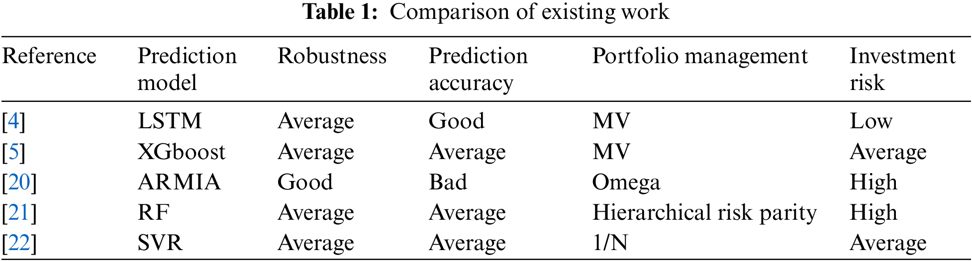
The construction of a smart beta strategy involves two major issues: stock selection optimization and weight optimization. Huang [3] created a stock selection model based on support vector regression (SVR) and genetic algorithms (GAs), in which SVR is used to predict each stock’s future return and GAs are used to optimize the model parameters and input features, and then weighted the top-ranked stocks equally to create the portfolio. Wang et al. [4] proposed an optimal portfolio construction method based on long short-term memory (LSTM) networks and mean-variance (MV) models. Chen et al. [5] proposed a new portfolio construction method that used a hybrid model combining extreme Gradient Boosting (XGBoost) and an improved Firefly Algorithm (IFA) to forecast future stock prices and use the MV model for portfolio selection. Tripathy et al. [6] summarized the Harris Hawk Optimizer (HHO) method being used to perform parameter optimization of regression techniques, for example, SVR. Braik al. [7] proposed a hybrid crow search algorithm for solving numerical and constrained global optimization problems. Alzubi et al. [8] put forward an efficient malware detection approach to feature weighting based. Alzubi et al. [9] proposed an optimal pruning algorithm called the dynamic programming approach to improving the accuracy. Many researchers [9–12] employed these forecasting models for stock pre-selection before portfolio creation, random forest (RF), SVR, LSTM, deep multi-layer perceptron (DMLP), and convolutional neural network (CNN). They then integrated their return prediction results into advancing MV and omega portfolio optimization models, respectively. However, all these machine learning methods in portfolio formation are purely dependent on the point prediction outcomes of maximum likelihood estimates and historical volatility, neglecting the uncertainty of the forecast.

The uncertainty of forecasts is critical for investors [13]. If an investor believes that a stock is likely to rise in value, they will buy more of that stock, which is known as the “certainty effect” in behavioral finance. To make optimal decisions, investors can quantify risk by estimating the uncertainty of the outcome. Forecast uncertainty can indicate the forecast model’s confidence in the forecast results and has some ability to explain the forecast results. Since it relies on machine learning analysis and obtains more objective results, this paper considers forecast uncertainty to be an important factor to consider in a smart beta strategy. Probabilistic prediction is a type of uncertainty forecasting, which, compared to traditional point forecasting, yields not only maximum likelihood estimates but also information about their probability distributions, which can provide more comprehensive guidance for portfolio management. Investors can manage uncertainty exposure during investment management. The methods of probabilistic prediction can be broadly classified into Bayesian and non-Bayesian methods [14]. Bayesian models offer a mathematically grounded framework to reason about model uncertainty. By integrating predictions across the posterior, Bayesian approaches naturally provide predictive uncertainty estimates, but they have practical drawbacks when primarily concerned with predictive uncertainty. Exact solutions of Bayesian models are limited to simple models, and calculating the posterior distribution for more powerful models such as Neural Networks (NN) and Bayesian Additive Regression Trees (BART) is difficult. Furthermore, sampling-based inference necessitates some statistical knowledge, which limits the use of Bayesian approaches.

The non-Bayesian approach is simple to implement and parallelize, and it produces high-quality estimates of prediction uncertainty that are more suited to huge financial data sets. To improve the predictive uncertainty estimation capability of a single deterministic deep neural network (DNN), Liu et al. [15] presented the Spectral Normalized Neural Gaussian Process (SNGP). However, DNN’s ability to capture features of structured input data is limited, and prediction accuracy is low. Deep ensembles fit an ensemble of neural networks to the dataset and obtain predictive uncertainty by making an approximation to the Gaussian mixture arising out of the ensemble [16]. Moreover, deep ensembles can give overconfident uncertainty estimates in practice [17]. Natural gradient boosting (NGBoost) combines a multi-parameter boosting algorithm with the natural gradient to efficiently estimate how parameters of the presumed outcome distribution vary with the observed features. In comparison to existing probabilistic prediction approaches, NGBoost is appropriate for structured input data prediction, and it is simple to use, flexible, and capable of obtaining good uncertainty estimates, allowing it to effectively measure various real-time risks. NGBoost has also been used to predict temperature [18], short-term solar irradiance, and short-term wind power prediction models [19]. We summarized the existing research work in Table 1.

2  Methods

2.1 Portfolio Optimization Based on Probabilistic Forecasting

By using probabilistic forecasting, investors can learn about an asset’s predicted return r and probability distribution. The variance of the predicted return is denoted by σ2(σ2≥0).

Based on the probabilistic forecast results, n stocks from the feasible asset allocation domain are chosen to form a portfolio P={P1,P2,…,Pn}(Pi denotes stock i), corresponding to a predicted return of rP={r1,r2,…,rn} and X={x1,x2,…,xn} is the investor’s investment proportion in stock i(i=1…,n) (where xi≥0 and ∑i=1nxi=1), then the predicted return of P is Rp(X)=∑i=1nxiri, Cov(ri,rj) denotes the predicted return between Pi and Pj. The covariance of P is σP2=∑i=1n∑j=1nxixjCov(ri,rj).

The goal of portfolio management is to balance return and risk, and the Sharpe ratio indicates the excess return per unit of risk, with a higher Sharpe ratio indicating better portfolio performance, so this paper employs the Sharpe ratio as an objective function. Sharpe ratio is calculated by the following Eq. (1):

SR=rp−rfσp(1)

where rP denotes the forecasted return of the portfolio; rf denotes the risk-free return; σP denotes the standard deviation of the forecasted return of the portfolio; and rP−rf is the risk premium.

The Smart beta strategy uses the predicted values obtained from probabilistic forecasting to construct the portfolio and the probability distribution obtained from probabilistic forecasting to achieve asset allocation. The smart beta strategy translates to solving the optimization problem shown in Eq. (2).

{maxSR=Rp(X)−rfσps.t.∑i=1nxi=10≤xi≤1,∀i=1,2,…,n(2)

Consider the case where the portfolio only contains two stocks, and define Px∈P as the asset allocation that invests in P1 and P2 according to the weights of x and (1−x), respectively, to allocate the portfolio with the highest Sharpe ratio in the feasible asset allocation, i.e., ∀Px∈P:SR(RP(x))≤SR(RP(x∗)). Px’s predicted return and uncertainty level (risk level) are denoted by r¯(x) and σ(x), respectively.

The maximum predicted return is different for different levels of risk. The maximum forecast return that can be obtained for a given level of risk is the set of optimal portfolios. These optimal combinations will form a curve on the predicted value-volatility plane, which we call f(x)=(σ(x),r¯(x)). This curve depicts the relationship between expected returns and volatility for a variety of viable assets. where σ(x) and r¯(x) are as Eqs. (3) and (4):

σ2(x)=σp2=x2σ12+(1−x)2σ22+2x(1−x)Cov(r1,r2)(3)

r¯(x)=Rp(x)=xr1+(1−x)r2(4)

On the predicted value-volatility plane, the Sharpe ratio of an asset allocation is equal to the slope of the line connecting the risk-free asset to this asset allocation. To find the asset allocation with the largest Sharpe ratio, the line must be tangential to the curve and pass through the risk-free asset point.

The slope at portfolio Px is expressed in Eq. (5).

dRp(x)dσp=[r1−r2]x2σ12+(1−x)2σ22+2x(1−x)Cov(r1,r2)xσ12+(x−1)σ22+(1−2x)Cov(r1,r2).(5)

The Sharpe ratio of a portfolio is expressed in Eq. (6).

Sp:=Rp(x)−rfσp=xr1+(1−x)r2−rfx2σ12+(1−x)2σ22+2x(1−x)Cov(r1,r2).(6)

Let Eqs. (5) and (6) be equal and solve for

x=[r2−rf]Cov(r1,r2)−[r1−rf]σ22[r1−r2][Cov(r1,r2)−σ22]−[r2−rf][σ12+σ22−2Cov(r1,r2)](7)

that is, the optimal two stocks are assigned weights based on the predicted values, X={x1,x2}={x,(1−x)}.

2.2 Proposed Model: NGB-PF

As shown in Fig. 1, the NGB-PF model developed in this research is separated into three stages and based on probabilistic forecasting. The stock data is standardized in the data pre-processing stage. The probabilistic prediction stage involves predicting each stock’s future return based on historical data and the associated uncertainty information. Through the PF model, the portfolio optimization stage obtains asset allocation ratios and forms trading decisions using the uncertainty information received from the preceding step of probabilistic prediction.

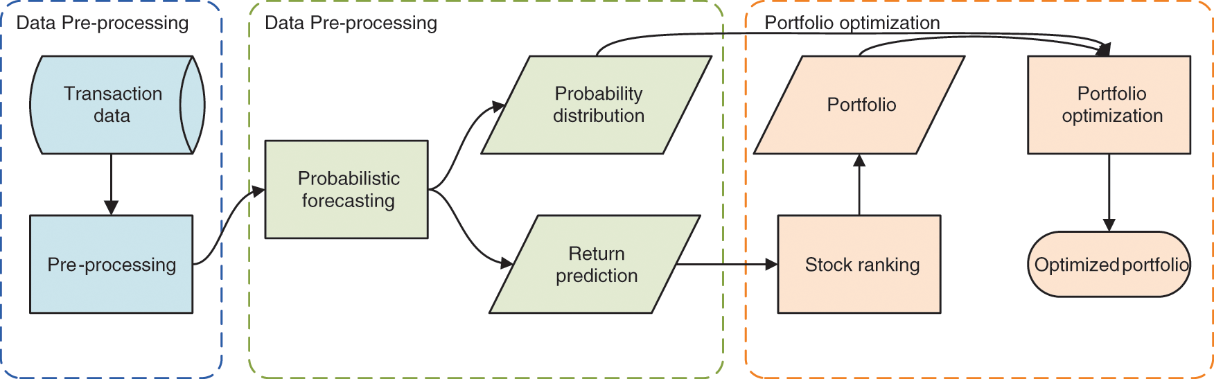
Figure 1: Flow chart of the proposed model

2.2.1 Data Pre-Processing

First, the stocks with suspension cases and small market capitalization in the dataset are removed. The obtained stock data may have disordered or missing values, so we need to operate sorting and adding missing values to obtain a complete and valid stock time series data set.

Due to the differences in the dimensionality of the time series features, the feature values need to be normalized. The normalization of each feature component is performed using the maximum minimization method. The normalized value of the eigenvalue x is expressed in Eq. (8).

x′=x−xminxmax−xmin(8)

2.2.2 Probabilistic Prediction

Since NGBoost is designed to be scalable and modular, it has base learners (e.g., decision trees), probability distribution parameters (e.g., normal distribution, Laplace distribution, etc.), and scoring rules (e.g., maximum likelihood estimation), it may employ flexible tree-based models for probabilistic prediction. The flowchart of NGBoost is shown in Fig. 2, which first passes the technical indicator x to the base learner (decision tree) to obtain a probability prediction with probability density Pθ(y|x) over the entire outcome space y. The model is then optimized by employing the maximum likelihood estimation function, which yields the calibrated uncertainty and point predictions as the scoring rule S(Pθ,y).

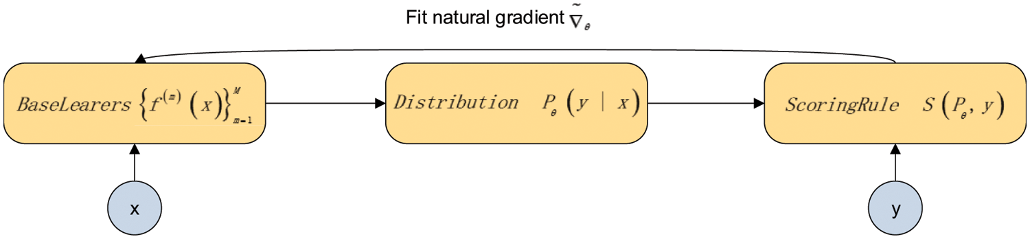
Figure 2: NGBoost model flow chart

The generalized natural gradient is the direction of the fastest ascent in Riemannian space, and it has the advantage of remaining invariant to parameters under different distributional changes. As a result, NGBoost employs natural gradient learning parameters, allowing the optimization problem to be parameterized-independent. Each base learner is permitted to fit the natural gradient in the framework of a gradient boost machine (GBM), and after scaling and additive combination, the parameters of the integrated model are acquired. For probabilistic prediction, the parameters of the final conditional distribution can be learned from the parameters of the integrated model. In standard prediction settings, the object of interest is an estimate of the scalar function E(y|x), where x is a vector of observed features and y is the prediction target. NGBoost generates a probability prediction with probability density Pθ(y|x) by directly predicting the parameter θ, and then the probability is determined so that the parameter satisfies the distribution of the observed feature vectors. The algorithm is made up of three modules: the base learner (f), the parameter probability distribution (Pθ), and the appropriate scoring rule (S).

A prediction y|x on a new input x is made in the form of a conditional distribution Pθ, whose parameters θ are obtained by an additive combination of M base learner outputs (corresponding to the M gradient boosting stages) and an initial θ(0). Note that θ can be a vector of parameters (not limited to scalar-valued), and they completely determine the probabilistic prediction y|x. f(m) refers to a collection of base learners of stage m, one for each parameter. Each base learner f(m) takes x as input to calculate the prediction parameter for x. When using the normal distribution in the experiment (θ=(μ,log⁡σ)), there are two base learners fμ(m) and flog⁡σ(m) at each stage, uniformly expressed as: f(m)=(fμ(m),flog⁡σ(m)). The predicted output is scaled by a stage-specific scaling factor ρ(m) and a common learning rate η. It is expressed in Eq. (9).

y|x∼Pθ(y|x),θ=θ(0)−η∑m=1Mβ(m)⋅f(m)(x)(9)

The scoring rule S is the gradient over the probability distribution Pθ concerning the parameter θ, denoted as ∇S(θ,y), where θ is the parameter and y is the predicted target, which is the direction of the most rapid ascent, and a very small amount of moving the parameter in the direction of this gradient increases the scoring rule by the most, which is expressed in Eq. (10),

∇∼S(θ,y)∝limε→0argmaxd:Ds(Pθ∥Pθ+d)=εS(θ+d,y)(10)

where d is the gradient’s change in direction and D is the divergence.

By solving the above optimization problem, the natural gradient of the problem can be obtained by Eq. (11):

∇∼S(θ,y)∝IS(θ)−1∇S(θ,y)(11)

where Is(θ) is the Riemannian measure of the statistical manifold at θ, which is derived from the scoring rule S. Let S = L, where L is the parameter estimate used for the scoring rule S. The NGBoost algorithm uses the maximum likelihood estimation by default. Solving the above optimization problem yields Eq. (12):

∇∼L(θ,y)∝IL(θ)−1∇L(θ,y)(12)

where IL(θ) is the amount of Fisher information from the observations about Pθ, defined as Eq. (13):

IL(θ)=Ey∼Pθ[∇θL(θ,y)∇θL(θ,y)T]=Ey∼Pθ[−∇θ2L(θ,y)](13)

When natural gradients are used to learn the parameters, the optimization problem becomes parameterization independent and has more efficient and stable learning dynamics than when only gradients are used. Additionally, the fast sort time complexity of a list of e elements is O(elog2⁡e). So we can calculate the time complexity of NGboost as O(Kdnlog2⁡n), where K means the total number of base learners and d represents the maximum depth of the base learners.

2.2.3 Model with Probabilistic Forecasting (PF)

According to the forecasted returns, the stocks are ranked in descending order, and the top k stocks are chosen to form the portfolio. Any two of these stocks are chosen, and the allocation weights are calculated using the formula (11). When the third stock is added, the first and second stocks become a new stock M with a forecast return rM=xr1+(1−x)r2 and a variance σM2=x2σ12+(1−x)2σ22+2x(1−x)cov(r1,r2). From the formula derived above, the weights of the updated portfolio can be obtained as X={x1,x2,x3} respectively, which is expressed by Eqs. (14) and (15).

{x1=xMxx2=xM(1−x)x3=1−xM(14)

xM=[r3−rf]Cov(rM,r3)−[rM−rf]σ32[rM−r3][Cov(rM,r3)−σ32]−[r3−rf][σM2+σ32−2Cov(rM,r3)](15)

Similarly, the allocation weights for k stocks can be obtained. Additionally, the time complexity of this algorithm is O(k3).

2.3 Benchmark Models and Baseline Strategies

2.3.1 Prediction Benchmark Models: LSTM and Bayesian-LSTM (BLSTM)

This paper chooses two representative machine learning models for financial time series forecasting to benchmark the models proposed in this paper: LSTM and Bayesian-LSTM. In the following paragraphs, this paper will explain the rationale behind each model.

LSTM is a classical point prediction model that gives the predicted value at a given moment and is widely used for financial time series forecasting. LSTM is a recurrent neural network that was proposed to overcome the limitations of recurrent neural networks and preserve long-term information [23]. This property is primarily based on the hidden layer’s storage unit. LSTM neural networks typically have three layers: an input layer, a hidden layer, and an output layer. In comparison to traditional neural networks, the control gate structure in LSTM neural networks can effectively simulate long-term dependencies in time series, allowing for the effective transmission of stock history data.

The Bayesian-LSTM model combines Bayesian principles with deep neural networks to make probabilistic predictions. Instead of using point estimates for the model parameters, it generates distributions for each parameter, and from the distribution of the parameters, the probability distribution of each value of the model output can be obtained, providing important uncertainty information related to prediction.

2.3.2 Baseline Strategy for the Portfolio

(1)   Mean-variance model

Markowitz’s [24] MV model serves as the foundation for portfolio optimization. Investment return and risk are quantified in this model by expected return and variance, respectively, and the model seeks to strike a balance between maximizing return and minimizing risk. A rational investor will always seek the lowest risk for a given expected return or the highest return for a given risk, and will select an appropriate portfolio to maximize expected utility, which is expressed by a typical multi-objective optimization formula, which is expressed by Eq. (16):

{min∑i=1n∑j=1nxixjσijmax∑i=1nxiμis.t.∑i=1nxi=10≤xi≤1,∀i=1,2,…,n(16)

where σij is the covariance between asset i and asset j, xi and xj are the proportion of investment in asset i and asset j, respectively, and μi is the expected return on asset i.

(2)   Equal-weighted model (1/N)

Due to the ease of implementation of this basic allocation method, investors continue to use the equally weighted portfolio (1/N) [25] as a benchmark for comparing the performance of many portfolios described in the literature in addition to the MV model.

3  Experiments and Results

This section first presents the variables chosen for the experiment and the data used, as well as the prediction results of the various models in stock forecasting throughout the test period. Following that, trading simulations are run to compare the performance of various models and strategies in daily trading investments with no transaction fees.

3.1 Data and Input Indicators

Due to the continuity of financial stock data, the sample data should cover a sufficiently long period. The constituent stocks of the CSI 300 are chosen based on volume and total market capitalization, and they are distinguished by their large size, relative stability, and adequate liquidity. Following the data pre-processing, 62 stocks are used in the experiment. The data from December 8, 2016, to May 31, 2019, were selected for the experiment and were obtained from JoinQuant. The data from December 8, 2016, to November 30, 2017, for 243 days were used as the experimental data set. The data from December 1, 2017, to May 31, 2018, for 120 days were used as the validation set, and the data from June 1, 2018, to May 31, 2019, for 243 days were used as the test set.

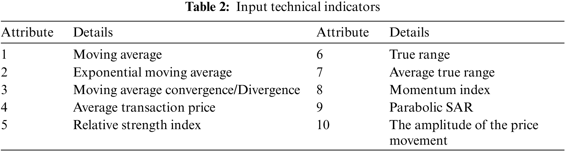
In this paper, 10 technical indicators are selected as inputs for stock forecasting: moving average (MA), exponential moving average (EMA), moving average (MA), moving average convergence/divergence (MACD), average transaction price (ATP), relative strength index (RSI), true range (TR), average true range (ATR), momentum index (MoM), parabolic SAR and amplitude of the price movement (ALT). Table 2 summarizes the selected input technical indicators.

3.2 Comparison of Predicted Results

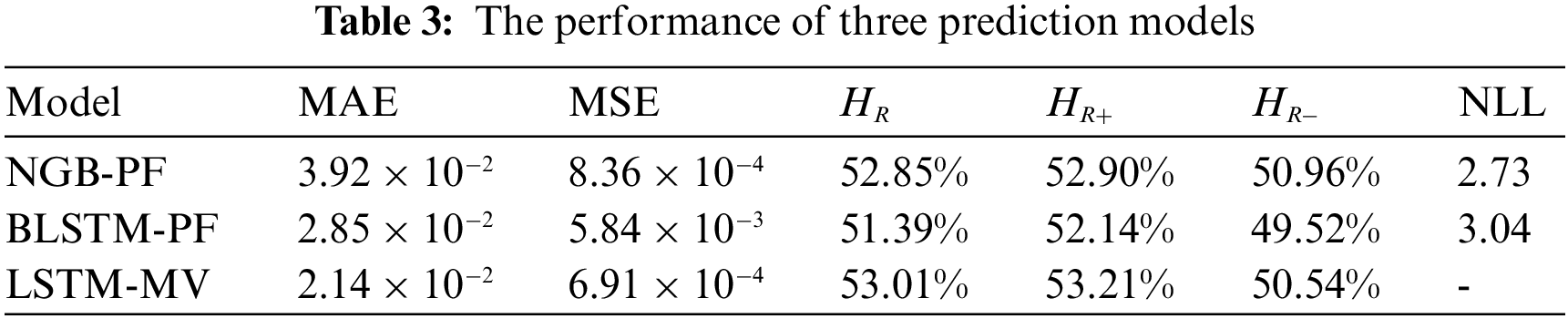
Six metrics are used in this paper to comprehensively measure the performance of different models in the stock forecasting process: mean absolute error (MAE), mean square error (MSE), HR, HR+, HR− and NLL. MSE usually represents the dispersion of the forecast outcome and MAE represents the deviation of the forecast outcome. In addition, HR denotes the total hit rate, HR+ means the accuracy of positive prediction and HR− means the accuracy of negative prediction. The negative mean log likelihood (NLL) is a popular metric for analyzing forecast uncertainty and is an effective scoring method for quantifying the quality of probabilistic forecasts [19]. Smaller MAE, MSE and NLL values and larger HR, HR+, and HR− values indicate better performance. These metrics are defined as Eqs. (17)–(22):

MAE=1n∑i=1n|yi−y^i|(17)

MSE=1n∑i=1n(yi−y^i)2(18)

HR=Counti=1n(yiy^i>0)Counti=1n(yiy^i≠0)(19)

HR+=Counti=1n(yi>0 AND y^i>0)Counti=1n(y^i>0)(20)

HR−=Counti=1n(yi<0 AND y^i<0)Counti=1n(y^i<0)(21)

NLL=log⁡P^θ(y|x)(22)

where yi^ denotes the forecast price, yi denotes the actual price, and n denotes the number of forecast days.

First, the performance of the three prediction models is compared, and as shown in Table 3, the error of NGB-PF is the smallest among the three models, which means that the prediction accuracy of NGB-PF is higher. The NLL index of NGB-PF is 2.73 greater than that of BLSTM-PF, showing that NGB-PF has a comparatively high quality in predicting uncertainty. In conclusion, NGB-PF outperforms the other models in the stock return prediction process.

3.3 Comparison of Backtest Results

This section will determine the proper cardinality of the portfolio and evaluate the effectiveness and superiority of the proposed NGB-PF.

Most studies related to the portfolio formation of individual investors focus only on about 10 assets [26–28]. Oreng et al. [29] found that portfolios with 7 assets outperformed those with another number of stocks. Therefore, in this paper, we choose 7 assets to form a portfolio and use four indicators, annualized mean return, annualized standard deviation, annualized Sharpe ratio, and annualized Sortino ratio, to assess the performance of the portfolio. The Sharpe ratio is a comprehensive indicator that can consider both return and risk. The Sortino ratio can distinguish between good and bad fluctuations. A larger Sharpe ratio and Sortino ratio indicate better performance.

According to Panel A of Table 4, NGB-PF has the highest annualized return of 0.29, while LSTM-MV has the lowest annualized return of 0.1703. NGB-PF has the lowest volatility of 0.2746, while BLSTM-1/N has the highest volatility. The annualized Sharpe ratio of NGB-PF is the highest, as is the Sortino ratio. The ability of NGBoost to effectively capture the features of the structured input dataset and the ability of the PF model to adjust the positions of the smart beta strategy by taking into account forecast uncertainty when performing asset allocation gives the proposed approach in this paper the best overall performance. The LSTM-1/N model, on the other hand, performs relatively poorly due to its lack of flexibility in allocating resources.

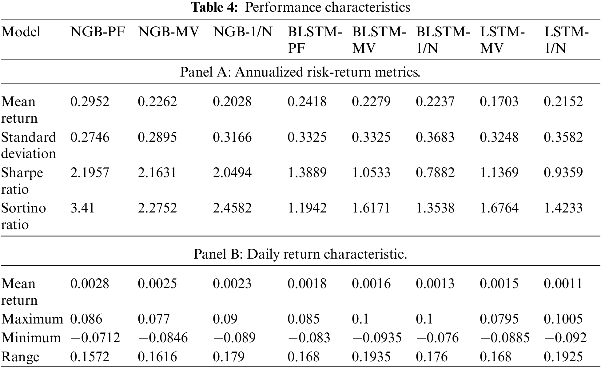
As shown in Panel B of Table 4, the mean return of NGBoost models is 0.2414, which is generally better than that of the model using BLSTM (0.2311) and LSTM (0.1927). This is highly related to the high robustness of the NGBoost models in dealing with uncertain system data. Also, as shown in Fig. 3, the average standard deviation of the MV-based position optimization method is 0.3156. However, it can reduce the risk compared with the 1/N models (average standard deviation of 0.3477). But the PF models proposed in this paper (standard deviation of 0.2746) gives the best results.

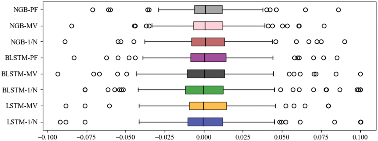
Figure 3: Box plot of the daily returns

It can be seen that although NGBoost-1/N leads in cumulative returns for the year, the magnitude is not large. And its returns are not as good as BLSTM-1/N from Q1-2019 to Q2-2019. But on the other hand, NGBoost-1/N has less overall volatility and better consistency. The base learner of NGboost is a decision tree, which is very tolerant of data missing. As an ensemble learning method, NGBoost reduces overfitting by returning the probability distribution method for each prediction. BLSTM and LSTM also have good accuracy, but the neural networks have more learning parameters, which causes them to be less robust than NGBoost. It also validates the view of Fischer et al. [26].

The cumulative return curve derived from the prediction model integrated with the MV model is shown in Fig. 5. Fig. 5 shows that the NGB-MV model has the best cumulative return of 60.42%, the cumulative return of the BLSTM-MV model is 38.83% and the LSTM-MV model has the lowest cumulative return of 35.34%. Compared to Fig. 4, the returns of all three algorithms have improved, and the volatility has decreased. The MV algorithm estimates the future risk from the historical volatility and optimizes the portfolio positions accordingly. Due to the continuity of stock styles, the MV algorithm can serve to reduce risk and increase efficiency, but the method may experience degradation in performance over time when rapid switches in market styles occur.

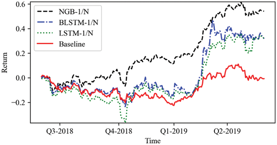
Figure 4: Cumulative returns by 1/N models

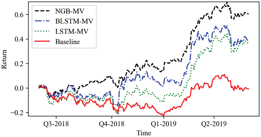
Figure 5: Cumulative returns by MV models

As shown in Fig. 6, the NGB-PF model has a constantly growing cumulative return, reaching a maximum of 67.1%, but the NGB-MV and NGB-1/N models have maximum cumulative returns of just 60.4% and 54.08%, respectively. The cumulative return of BLSTM-MV is only 3.49% higher than that of LSTM-MV, and the difference is not significant. The cumulative return achieved by the BLSTM-PF model is 44.0%, which is also higher than the cumulative return achieved by the BLSTM-MV, which is 38.83%. The NGBoost and BLSTM algorithms combined with the PF model further improve the gain and reduce the volatility compared to using the MV model. The PF model uses the probability distribution data of the prediction results, which requires the prediction model itself to have the ability of probability prediction. Since LSTM does not have this capability, the PF model cannot be used. The analytical solution of the position optimization scheme derived from Section 2.1, combined with the excellent probability prediction capability of NGBoost, can help the smart beta strategy maintain transparency while being able to better control risk and improve returns.

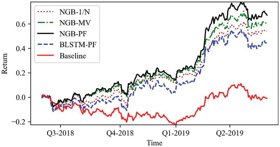
Figure 6: Cumulative returns by PF models

4  Conclusions and Discussion

The main focus of this paper is to propose an improved smart beta strategy for portfolio management. The main contributions of this work are:

1.    This paper uses the quantitative uncertainty of prediction to determine the allocation share. This investment allocation has endogenous logic and is an objective portfolio method based on confidence in the prediction value, which conforms to modern people’s investment psychology.

2.    There are two outputs of probability prediction: predictive value and probability distribution, both of which will be used to allocate the weight of portfolio investment. This paper compares the prediction ability of NGBoost, BLSTM and LSTM in stock return prediction through experiments. Six indicators are used to comprehensively measure the performance of different models in the process of stock return prediction. The experimental results show that the NGB-PF model has the smallest prediction error and the highest prediction accuracy among these models, which indicates that NGBoost is suitable for stock return prediction.

3.    The quality of forecast uncertainty will also affect the performance of the portfolio constructed by using forecast uncertainty. Through experimental verification, the cumulative yield of the BLSTM-PF model with low prediction uncertainty is 23.1% lower than that of the NGB-PF model. To further measure the effectiveness of the PF model, we compared it with the benchmark model, MV model and 1/N model and found that the PF model can more reasonably allocate the weight of the portfolio when using the prediction results of the same prediction model, thus promoting the steady growth of income. The cumulative rate of return of the NGB-PF model reached 67.1% at the highest, thanks to its use of prediction uncertainty to guide portfolio management.

This study also has some practical implications for individual investors, as this approach can help them make investment decisions more effectively, reduce risk, and ensure the safety and profitability of their investments. Although this study has some research implications, more research can be conducted. For example, the input characteristics could take into account some other external environmental factors such as news, government policies, interest rates, etc. Besides, we still face challenges in improving the training efficiency of the algorithm. The NGBoost algorithm learns in a sequential form and does not support parallel computing, so it cannot take full advantage of multi-core computers to reduce the training time, which is a current limitation of the algorithm. Although it will not have much impact in the case of using daily data for analysis, it is indeed a problem worth investigating in the future.

Funding Statement: This work was supported by the National Natural Science Foundation of China [Grant Number 61902349].

Conflicts of Interest: The authors declare that they have no known competing financial interests or personal relationships that could have appeared to influence the work reported in the paper.

References

1. M. Agrawal, P. Shukla, R. Nair, A. Nayyar and M. Masud, “Stock prediction based on technical indicators using deep learning model,” Computers, Materials & Continua, vol. 70, no. 1, pp. 287, 2021. [Google Scholar]
2. K. M, S. Sankar, A. Kumar, T. Nestor, N. Soliman et al., “Stock market trading based on market sentiments and reinforcement learning,” Computers, Materials & Continua, vol. 70, no. 1, pp. 935, 2021. [Google Scholar]
3. C. -F. Huang, “A hybrid stock selection model using genetic algorithms and support vector regression,” Applied Soft Computing, vol. 12, no. 2, pp. 807–818, 2012. [Google Scholar]
4. W. Wang, W. Li, N. Zhang and K. Liu, “Portfolio formation with preselection using deep learning from long-term financial data,” Expert Systems with Applications, vol. 143, pp. 113042, 2020. [Google Scholar]
5. W. Chen, H. Zhang, M. K. Mehlawat and L. Jia, “Mean–variance portfolio optimization using machine learning-based stock price prediction,” Applied Soft Computing, vol. 100, pp. 106943, 2021. [Google Scholar]
6. B. K. Tripathy, P. K. Reddy Maddikunta, Q. -V. Pham, T. R. Gadekallu, K. Dev et al., “Harris hawk optimization: A survey onvariants and applications,” Computational Intelligence and Neuroscience, vol. 2022, pp. 2218594, 2022. [Google Scholar]
7. O. A. Alzubi, J. A. Alzubi, A. M. Al-Zoubi, M. A. Hassonah and U. Kose, “An efficient malware detection approach with feature weighting based on harris hawks optimization,” Cluster Computing, vol. 25, no. 4, pp. 2369–2387, 2022. [Google Scholar]
8. O. A. Alzubi, J. A. Alzubi, A. M. Al-Zoubi, M. A. Hassonah and U. Kose, “An efficient malware detection approach with feature weighting based on harris hawks optimization,” Cluster Computing, vol. 25, no. 4, pp. 2369–2387, 2022. [Google Scholar]
9. O. A. Alzubi, J. A. Alzubi, M. Alweshah, I. Qiqieh, S. Al-Shami et al., “An optimal pruning algorithm of classifier ensembles: Dynamic programming approach,” Neural Computing and Applications, vol. 32, no. 20, pp. 16091–16107, 2020. [Google Scholar]
10. Y. Ma, R. Han and W. Wang, “Portfolio optimization with return prediction using deep learning and machine learning,” Expert Systems with Applications, vol. 165, pp. 113973, 2021. [Google Scholar]
11. C. Zhao, X. Liu, J. Zhou, Y. Cen and X. Yao, “Gcn-based stock relations analysis for stock market prediction,” PeerJ Computer Science, vol. 8, pp. e1057, 2022. [Google Scholar]
12. Y. Chen, J. Wu and Z. Wu, “China’s commercial bank stock price prediction using a novel k-means-lstm hybrid approach,” Expert Systems with Applications, vol. 202, pp. 117370, 2022. [Google Scholar]
13. B. Rossi and T. Sekhposyan, “Macroeconomic uncertainty indices based on nowcast and forecast error distributions,” American Economic Review, vol. 105, no. 5, pp. 650–655, 2015. [Google Scholar]
14. T. Duan, A. Anand, D. Y. Ding, K. K. Thai, S. Basu et al., “Ngboost: Natural gradient boosting for probabilistic prediction,” in Proc. PMLR, Vienna, Austria, pp. 2690–2700, 2020. [Google Scholar]
15. J. Liu, Z. Lin, S. Padhy, D. Tran, T. Bedrax Weiss et al., “Simple and principled uncertainty estimation with deterministic deep learning via distance awareness,” Advances in Neural Information Processing Systems, vol. 33, pp. 7498–7512, 2020. [Google Scholar]
16. H. Zhang, L. Huang, C. Q. Wu and Z. Li, “An effective convolutional neural network based on smote and Gaussian mixture model for intrusion detection in imbalanced dataset,” Computer Networks, vol. 177, pp. 107315, 2020. [Google Scholar]
17. R. Rahaman, “Uncertainty quantification and deep ensembles,” Advances in Neural Information Processing Systems, vol. 34, pp. 20063–20075, 2021. [Google Scholar]
18. T. Peng, X. Zhi, Y. Ji, L. Ji and Y. Tian, “Prediction skill of extended range 2-m maximum air temperature probabilistic forecasts using machine learning post-processing methods,” Atmosphere, vol. 11, no. 8, pp. 823, 2020. [Google Scholar]
19. Y. Li, Y. Wang and B. Wu, “Short-term direct probability prediction model of wind power based on improved natural gradient boosting,” Energies, vol. 13, no. 18, pp. 4629, 2020. [Google Scholar]
20. J. -R. Yu, W. -J. P. Chiou, W. -Y. Lee and S. -J. Lin, “Portfolio models with return forecasting and transaction costs,” International Review of Economics & Finance, vol. 66, pp. 118–130, 2020. [Google Scholar]
21. T. Kaczmarek and K. Perez, “Building portfolios based on machine learning predictions,” Economic Research-Ekonomska Istraživanja, vol. 35, no. 1, pp. 19–37, 2022. [Google Scholar]
22. H. Yu, R. Chen and G. Zhang, “A svm stock selection model within pca,” Procedia Computer Science, vol. 31, pp. 406–412, 2014. [Google Scholar]
23. S. Hochreiter and J. Schmidhuber, “Long short-term memory,” Neural Computation, vol. 9, pp. 1735–1780, 1997. [Google Scholar]
24. H. Markowitz, “Portfolio selection*,” The Journal of Finance, vol. 7, no. 1, pp. 77–91, 1952. [Google Scholar]
25. F. Yang, Z. Chen, J. Li and L. Tang, “A novel hybrid stock selection method with stock prediction,” Applied Soft Computing, vol. 80, pp. 820–831, 2019. [Google Scholar]
26. D. P. Gandhmal and K. Kumar, “Systematic analysis and review of stock market prediction techniques,” Computer Science Review, vol. 34, pp. 100190, 2019. [Google Scholar]
27. B. Kocuk and G. Cornuéjols, “Incorporating black-litterman views in portfolio construction when stock returns are a mixture of normals,” Omega, vol. 91, pp. 102008, 2020. [Google Scholar]
28. S. Almahdi and S. Y. Yang, “An adaptive portfolio trading system: A risk-return portfolio optimization using recurrent reinforcement learning with expected maximum drawdown,” Expert Systems with Applications, vol. 87, pp. 267–279, 2017. [Google Scholar]
29. M. Oreng, C. E. Yoshinaga and W. Eid Junior, “Disposition effect, demographics and risk taking,” RAUSP Management Journal, vol. 56, no. 2, pp. 217–233, 2021. [Google Scholar]
Cite This Article
Copyright © 2023 The Author(s). Published by Tech Science Press.
This work is licensed under a Creative Commons Attribution 4.0 International License , which permits unrestricted use, distribution, and reproduction in any medium, provided the original work is properly cited.
Downloads
Citation Tools