Semantic Segmentation by Using Down-Sampling and Subpixel Convolution: DSSC-UNet

1  Introduction

Recently, as artificial intelligence research has been actively conducted, it is used in many fields from autonomous driving, medical image, robot vision, and video surveillance. Among them, segmentation becomes the main problem and assorted studies about it are being conducted. The problem of image segmentation can be classified by methods and goals. According to methods, there are 10 categories based on the model architectures. These are fully convolutional networks (FCN), Convolutional models with graphical models, Encoder-decoder based models, etc… [1]. According to goals, there are semantic, instance, and panoptic segmentation.

The goal of our research is semantic segmentation. It is a high-level problem that requires a complete understanding of the scene, not just looking at and classifying images. The purpose of semantic segmentation classifies all pixels of the input image into the corresponding class. In other words, pixel-level labeling is performed on all image pixels by using a series of object categories such as people, car, sky, tree, etc. The important problems in semantic segmentation are recognition of small objects, maintenance of detailed context of images, and localization of objects in images [1]. They are all related to segmentation performance. Several methods have been studied to solve these problems. In the convolution network (CNN) with the graphical model, Conditional Random Fields (CRFs) utilizes more context to solve the localization. It explored the “patch-patch” context (between image regions) and “patch-background” [2]. As a result, their model localizes segment boundaries more accurately. In the encoder-decoder based models, High-Resolution Net (HRNet) solves the loss of fine-grained image information [3]. This loss occurs through the encoding process. Encoder-Decoder models recover the high-resolution representations. However, HRNet maintains high-resolution representations by connecting the high-to-low convolutions streams in parallel and exchanging the information repeatedly between resolutions. As a result, it improves segmentation accuracy and is used as a backbone in recent models. In the multiscale and pyramid network-based model, Pyramid Scene Parsing Network (PSPN) utilizes the global context representation of a scene [4]. This means it captures both local and global context information of feature maps. It extracts the multiple patterns using a residual network (ResNet), with a dilated network. PSPN can improve the segmentation of small objects in a scene. And its idea, multiscale, is used in recent models such as DeepLabv3.

Early semantic segmentation studies applied deep neural networks often used for classification, such as AlexNet [5], VGGNet [6], and GoogLeNet [7] to the segmentation [8]. After that research, deep learning-based technology has developed rapidly in semantic segmentation [1]. Particularly, the deep learning-based semantic segmentation methods using Convolutional Neural Networks (CNN) are being studied. Representative methods are Fully Convolutional Networks (FCN) [8], U-Net [9], and SegNet [10]. However, these methods had several shortcomings [1]. In FCN, it is too computationally expensive for real-time inference. And it is hard to account for global context information efficiently and generalize it to 3D images. In U-Net, it lacks context information extracted from the encoder, resulting in incorrect or unsuccessful segmentation of the object. In SegNet, it has a limitation in that small objects in the image are not well classified. Motivated by these problems, we think we can minimize the loss that can occur when training detailed information on images that affect semantic segmentation and improve segmentation performance by using more context for training. Additionally, we think parameter-free subpixel convolution can reduce training time when it applies to the decoder.

In this paper, it proposed a new encoder-decoder based network to solve these problems: Down-Sampling and Subpixel Convolution U-Net (DSSC-UNet). It is based on U-Net, which used down-sampling instead of pooling operation with context loss. Also, it used the subpixel convolution, which was proposed by Efficient Sub-Pixel Convolutional Neural Network (ESPCN), instead of transposed convolution during image expansion. We think that feature maps of the down-sampling have more information than max pooling because of keeping the Nyquist theorem and extracting the latent information. The Nyquist theorem is that a signal can be restored to its original signal by sampling it at regular intervals, twice the frequency of the highest frequency contained in that signal. Based on this idea, this paper used two down-sampling maps of each feature for making noise robust. In addition, it also used two other diagonal elements for the skip connection. That is, our proposed method aims to minimize the loss of information and make noise robust to perform semantic segmentation with as much latent information as possible to increase segmentation accuracy.

This paper conducted experiments for comparing the performance of the base method (U-Net) and DSSC-UNet. The experiments were conducted 15 times using the cityscapes dataset. As a result of it, DSSC-UNet showed an increase in segmentation performance by about 4% compared to U-Net. The test result shows significant differences.

2  Related Work

2.1 Fully Convolution Network (FCN)

Fully convolution network (FCN) is a modified version of the CNN-based models (AlexNet, VGGNet, GoogLeNet) used in the existing classification to suit the purpose of semantic segmentation. It can be divided into three courses: Convolutionalization, Deconvolution, and Skip Architecture [8]. Regardless of the internal structure, the classification models consist of Fully Connected Layer (FC layer) for the fundamental goal of the model. This configuration is to extract the characteristics of the image using convolution from the input layer to the middle of the network and classifies the characteristics using the FC layer from the output layer part. However, from the viewpoint of semantic segmentation, there is a limitation of the FC layer. As a limitation, the location information of the image disappears, and the size of the input image is fixed.

To solve these limitations, FCN replaces the FC layer with Convolution. Through convolutionalization, the output feature map can contain the location information of the original image. However, compared to pixel-by-pixel prediction, the final purpose of semantic segmentation, FCN’s output feature map is too coarse. Therefore, it is necessary to convert the coarse map into a dense map close to the original image size. FCN used two methods: Bilinear interaction and Deconvolution to obtain dense prediction from a coarse feature map. However, the predicted dense map is still coarse because there is a lot of lost information. FCN solved this with Skip Architecture, which combines semantic information of Deep & Coarse layers with apparent information about the Shallow & Fine layers [8]. FCN was the basis for subsequent Semantic Segmentation methodologies. However, small objects can be ignored or perceived as unusual when it uses the restricted field. Also, large objects can be perceived as small objects or inconsistent results. In addition, there was a problem that the results were not accurate by using the method of restoring the reduced resolution through upscaling [11].

2.2 U-Net

U-Net is a fully convolution network (FCN)-based model proposed for image segmentation in the biomedical field. It consists of a network for obtaining overall context information of an image and a network for accurate localization [9]. And it proposed a method of combining shallow feature maps with deep feature maps using FCN’s concept of skip architecture. Despite better results than FCN in the medical field, U-Net lacks context information extracted from encoders, wrong segmentation of objects, or failure occurs. These problems interfere with the recognition of the location and motion of objects in autonomous vehicles, which are applications, and increase errors in the location and size of lesions in medical image analysis [12].

The network structure of U-Net is symmetrical and divided into the contracting path and the expansive path. The purpose of the contracting path is to capture the context in the input image. The expansive path upscales the context of feature maps captured in the contracting path and combines them with the information through skip connection. Its purpose is to make the localization more accurate. One example of the U-Net architecture sees Fig. 1.

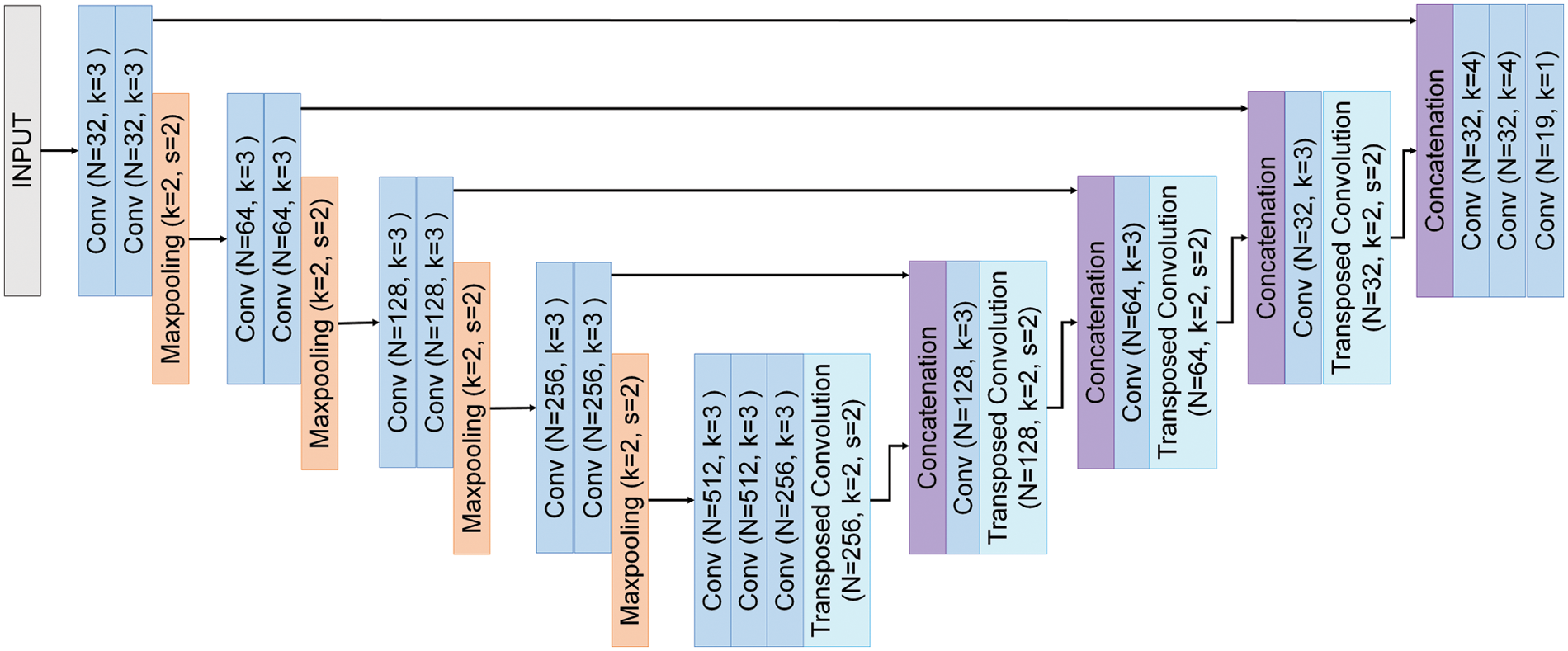
Figure 1: U-Net architecture

The contracting path consists of four blocks, each of them consisting of two 3 * 3 convolutions (same convolution), each followed by a Leaky Rectified Linear Unit (ReLU), Batch normalization, and Max Pooling. Max Pooling has a 2 * 2 kernel size and stride of 2. The number of channels in the blocks is initially 32 and doubles each time it moves to the next block. In the middle of the model, two 3 * 3 convolutions (same convolution) with 512 channels serve as the bottleneck. The expansive path consists of four blocks, each of them consisting of 3 * 3 convolution (same convolution), transposed convolution, and concatenation. Excepting concatenation operation, each is followed by a ReLU and Batch normalization. Transposed convolution has a 2 * 2 kernel size and stride of 2. The number of channels in the blocks is initially 512 and divided by 2 each time it moves to the next block. The output feature map of the last transposed convolution goes through two 4 * 4 convolutions (same convolution), each followed by dropout, and then adjusts the channels of the feature map to the same number of label classes through 1 * 1 convolution (same convolution).

The contracting path is the process of capturing the essential context of input images. Max pooling, which is a key operation of the contracting path, is a pooling operation that calculates the maximum value for patches of a feature map and uses it to create a pooled feature map. Max pooling does not have parameters for learning. This reduces the complexity of the model, thereby reducing the memory resources and speeding up. Because max pooling reduces parameters, it reduces computation, saving hardware resources, speeding up learning time, and suppressing overfitting to reduce the expressiveness of the network. Also, the result of pooling does not affect the number of channels, so the number of channels is maintained (independent) and even if there is a shift in the input feature map, the result of pooling has a slight change (robustness). In addition, information that captured the essential context of input images is delivered to upscaling process using a skip connection for preserving the structure and objects in the original image.

The expansive path is the process of upscaling feature maps. Key operations of the expansive path are transposed convolution and concatenation. Transposed convolution is to expand the size of an image. Like general convolution, it has parameters of padding and stride. If you do a general convolution with the values of stride and padding, you will create the same spatial dimension as the input. Given i,k,p,s of input, kernel, padding, and stride in a typical convolution layer, the length of the output o follows the formula below Eq. (1).

o=i−k+2ps+1(1)

Transposed convolution consists of three steps. At first, this operation dilates the input tensor with zero insertion. The input tensor is transformed into the tensor that consists of inserting d−1 zeroed rows and columns between each couple of rows and columns of it by using a dilation rate d. In U-Net, the dilation rate is set to s. In the second step, the tensor is padded with p′=k−p−1. In the third step, this operation performs general convolution with a stride of 1. That is, transposed convolution does the convolution with the finally transformed input tensor.

Concatenation operation combines deep, coarse, semantic information and shallow, fine, appearance information through skip architecture [8]. Since the semantic feature map has already lost a lot of information during reducing the size of the image, expanding this by using the transposed convolution results in coarse information that has summarized information. To solve this problem, U-Net used a skip connection in FCN [8]. This passed the fine feature maps, which is before the image reduction (max pooling) of the contracting path, to the symmetric expansive path. As a result, this can utilize coarse and fine information for the segmentation.

2.3 Subpixel Convolution

Subpixel convolution is the upscaling method that is proposed as Efficient Sub-Pixel Convolutional Neural Network (ESPCN) in the super-resolution [13]. Before ESPCN, the existing methods in super-resolution up-sample the image using bicubic interpolation and then apply a convolutional network [14]. However, ESPCN applies convolutional networks and then up-samples the image using a subpixel convolution. Unlike existing interpolation methods, the subpixel convolution layer up-samples feature maps by using their depth of them. This method has more representation power than existing methods [14]. Fig. 2 shows the subpixel convolution.

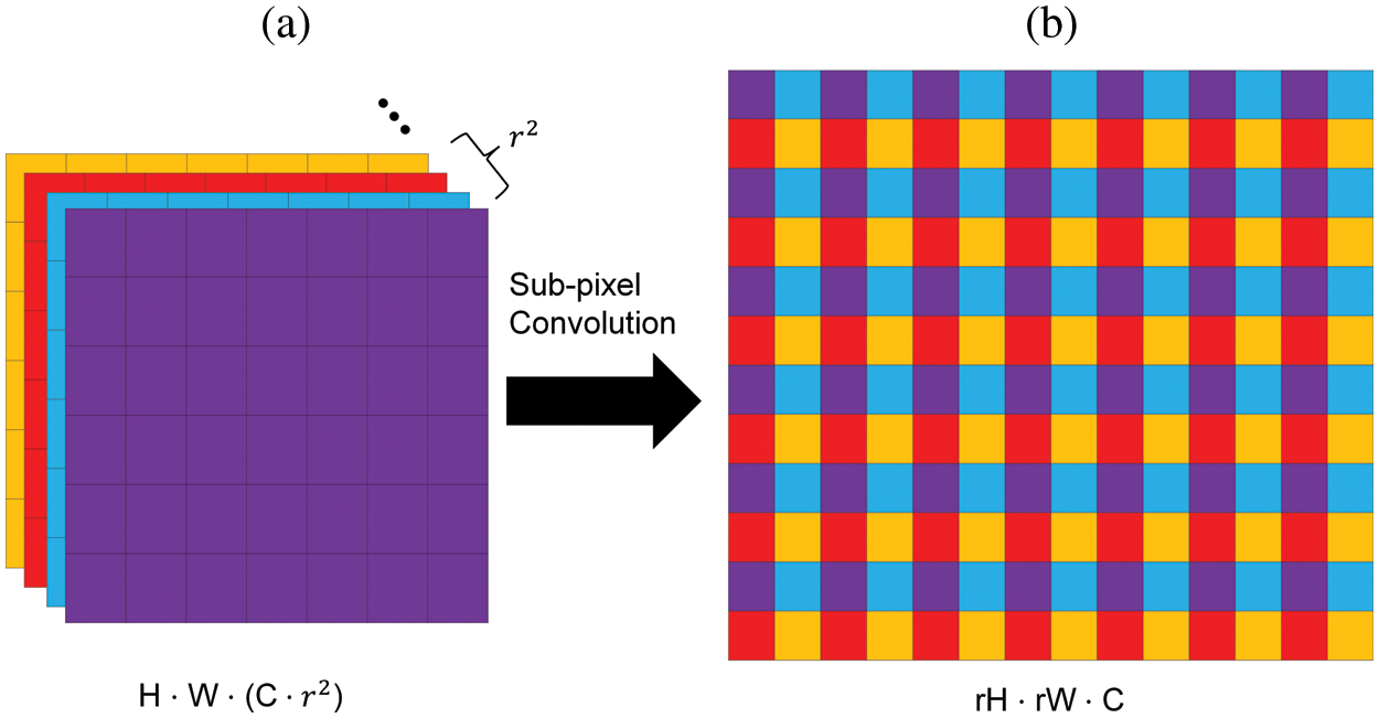
Figure 2: Subpixel convolution in efficient sub-pixel convolutional neural network (ESPCN). (a) Feature maps before subpixel convolution. (b) Feature map after subpixel convolution

Subpixel convolution makes the original image of size r2 × H × W by an image of size 1 × rH × rW to create the high-resolution image. As a result, it is upscaled by r times in each direction. For example, see the 4 color feature maps of the left in Fig. 2. After subpixel convolution, those look like the right of Fig. 2.

3  Proposed Network Architecture

This paper shows our proposed model (DSSC-UNet) in Fig. 3. It is based on the U-Net’s encoder-decoder and symmetric structure. It can be divided into two parts like U-Net: the contracting path that captures the context in the feature maps when reducing them and the expansive path that captures the accurate localization of the class when expanding them.

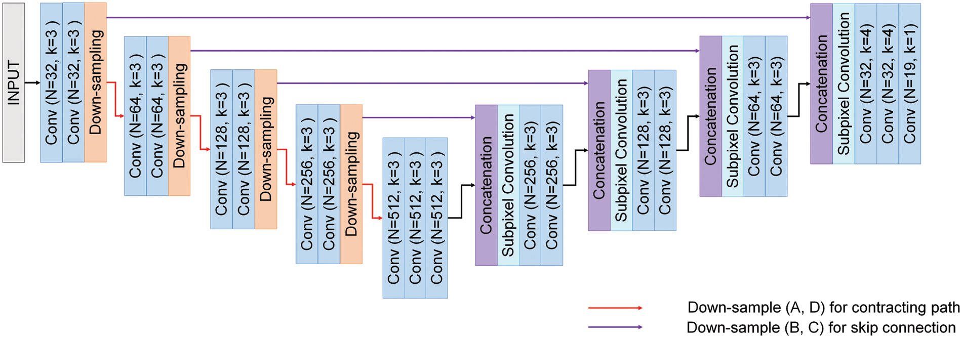
Figure 3: Proposed model (DSSC-UNet)

The contracting path consists of four blocks, each of the blocks consists of two 3 * 3 convolutions (same convolution) and sampling, each convolution followed by a Leaky Rectified Linear Unit (ReLU), Batch normalization (BN). The number of channels in the blocks is initially 32 and doubles each time it moves to the next block. The contracting path’s final channels are 512. And the bottleneck layer is between the contracting path and the expansive path. It consists of one 3 × 3 convolution (same convolution). The expansive path consists of four blocks, each of the blocks consists of two 3 × 3 convolutions, concatenation, and subpixel convolution. Each convolution is followed by ReLU, BN. The number of channels in the blocks is initially 512 and divided by 2 each time it moves to the next block. The expansive path’s final channels are 32. The final feature map of the expansive path passes through two 4 × 4 convolutions (same convolution) and then goes through a 1 × 1 convolution (same convolution). At the final layer, a 1 × 1 convolution is used to map each 32-component feature vector to the desired number of classes. There are 20 convolutional layers in the network. This paper called our proposed network: DSSC-UNet (Down-Sampling and Subpixel Convolution U-Net).

U-Net used the max pooling operation for feature map reduction in the contracting path. This may lose sensitive information of them. It means that detailed information on the feature maps might be lost because the max pooling summarizes them. To solve this problem, this paper replaced the max pooling operation with down-sampling. It was shown in Fig. 4.

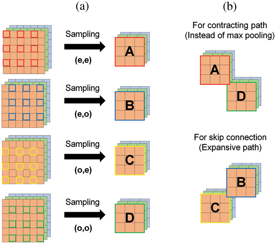
Figure 4: Down-sampling operation. (a) The feature maps before and after sampling. (b) Feature maps for contracting path and skip-connection

Max pooling operation has a fundamental problem of losing detailed information when reducing the feature maps. So, this paper uses sampling instead of max pooling to avoid this problem. It is different from the max pooling operation. In deep learning, the sampling can be divided into two categories: down-sampling and up-sampling. Down-sampling is the process of reducing the size of data. If the feature maps down-sample with stride 2, four kinds of them are created. They are shown in Fig. 4a. It will use each two feature maps for contracting path and skip-connection. They are shown in Fig. 4b.

As shown in Fig. 4a, the A is a feature map that starts at [0, 0] and consists of pixels located in indexes with even rows and even columns. The B is a feature map that starts at [0, 1] and consists of pixels located in indexes with even rows and odd columns. The C is a feature map that starts at [1, 0] and consists of pixels located in indexes with odd rows and even columns. The D is a feature map that starts at [1, 1] and consists of pixels located in indexes with odd rows and odd columns. The size of them is half of the input feature maps, but the size of batch and channels is maintained. In U-Net, summarized data configured with maximum value are used to extract the feature. On the contrary to this, DSSC-UNet used two diagonally symmetric data summarized by sampling to extract features. That is, it uses more summarized data in feature extraction than U-Net. We expect that it will find more hidden features of input data and improve segmentation performance. In addition, the remaining feature maps of the sampling, not used for feature extraction in the contracting path, are passed through the skip connection as additional information for image restoration in the expansive path. As a result, sampling improves segmentation performance because it extracts more latent features than max pooling and makes noise robust.

In U-Net, transposed convolution expanded the size of the feature maps. However, it has the disadvantages of increasing the amount of computation due to increased parameters and generating checkerboard artifacts [15]. To solve this problem, this paper used subpixel convolution in DSSC-UNet. It restores the size of the original image by reconstructing the feature maps. Fig. 5 presented the expanding process using it. In Fig. 5, slicing performs preprocessing to connect the feature maps summarized in the contracting path to transfer from the skip connection. Its process is as follows. First, it divides the summarized feature maps A and D in half. Through this process, A and D are divided independently. Next, the transferred B and C are connected between A and D. The sequence of concatenation is A, B, C, and D. It is based on the channel axis. Finally, the result of the concatenation performs the subpixel convolution operation. It is restored to the size of the original image by subpixel convolution. The operation of the subpixel convolution has the advantage of reducing computational complexity because parameters do not generate.

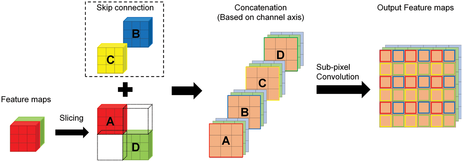
Figure 5: Expanding process using subpixel convolution operation

As a result, DSSC-UNet will restore as close as possible to the original image, minimizing the loss of detailed context of the image, unlike existing methods. Through this, we expect that it will improve the segmentation performance.

In summary, this paper can explain our algorithm in the three main steps: contracting path (encoding), bottleneck, and expansive path (decoding). The following summarized the algorithm of DSSC-UNet:

1.   Contracting path (encoding): Extract the hidden feature from the input data

1-1. Perform the input data with 3 × 3 convolution (same convolution), Batch Normalization (BN), and Leaky Rectified Linear Unit (ReLU) twice.

1-2. Divide the output feature maps into four kinds of them (A, B, C, and D) by down-sampling.

1-3. Send the A and D feature maps for the next encoding process. Keep the B and C feature maps for skip connection.

1-4. Repeat 1-1–1-3 from 4 times. Each iteration doubles the number of channels. The initial number of channels is 32.

2.   Bottleneck:

Perform the output feature maps through the last iteration of the contracting path with one 3 × 3 convolution (same convolution), BN, and ReLU. The number of channels is 512.

3.   Expansive path (decoding): Image restoration and expansion

3-1. Perform the output feature maps of the bottleneck layer with 3 × 3 convolution (same convolution), BN, and ReLU twice.

3-2. Concatenate the output feature maps with B and C that were stored in an empty list of the contracting path. When concatenating output feature maps to B and C, they are divided in half and concatenate B and C in the middle of the divided feature maps. When calling B and C for concatenation, they are called in reverse of the stored order in the list. In other words, the last stored B and C are called first. In addition, concatenation is based on the channel axis.

3-3. Expanding concatenated feature maps through the subpixel convolution.

3-4. Repeat 3-1–3-3 from 4 times. Each iteration halves the number of channels. The initial number of channels is 512.

3-5. After the last iteration of the expansive path, perform output feature maps with 4 × 4 convolution (same convolution), and ReLU twice. At last, performing 1 × 1 convolution maps each of the component feature vectors to the desired number of classes. In our network, the number of classes is 19.

4  Experiments

4.1 Dataset and Metric

During the evaluation, Cityscapes, a publicly available benchmark dataset, was used. It is a large-scale database with a focus on semantic understanding of urban street scenes [1]. It includes a variety set of stereo video sequences recorded in street scenes from 50 cities, with high-quality pixel-level annotation of 5 k frames in addition to a set of 20 k weakly annotated frames. It includes semantic and dense pixel annotations of 30 classes grouped into 8 categories (flat surfaces, humans, vehicles, constructions, objects, nature, sky, and void) [16]. Among the cityscapes dataset, LeftImg8bit and gtFine are used for evaluation. It includes 2975 train images and 500 validation images.

The data used in the training and validation have the same trainId for several classes. For training, labels with trainId of 255 or less than 0 are ignored so that they are not used for evaluation. Our experiments only use 19 categories for data classification. Additionally, various random transformations (random saturation/brightness change, random horizontal flip, random crop/scaling, etc…) are applied to increase the data to be used for training. Some transformations should be applied to both the input image and the target label map. When the image is turned over or cut, the same should be performed on the label map.

Representative metrics for segmentation models are pixel accuracy, mean pixel accuracy, intersection over union, mean intersection over union (Mean-IoU), precision/recall/F1 score, and dice coefficient. Among the metrics, this paper uses the mean intersection over union for measuring the performance of our proposed model (DSSC-UNet). Intersection over Union (IoU) is defined as an overlapping area between the predicted segmentation map and the ground truth and can be divided into their area of union. The following Eq. (2) is the formula of IoU, and each of A and B represents the predicted segmentation map and ground truth. It ranges between 0 and 1. Mean-IoU is defined as the average of the IoU and it can be obtained by averaging the results of the IoU calculation by class.

IoU=J(A,B)=|A∩B||A∪B|(2)

4.2 Hyper Parameters

In training, all input images are preprocessed to be 512 × 512 × 3. The number of classes to be classified in the data is 19. It used Adam optimizer to optimize all the network by setting β1 = 0.9, β2 = 0.999. The learning rate is set to 1e-3. It uses sparse categorical cross entropy to train the proposed model and sparse categorical accuracy to evaluate the performance of the trained model in the validation set. Additionally, before calculating the loss and accuracy, we except ignored labels from the predicted logit map and ground-truth label map to compare only the considered class. This paper used Tensorflow to implement our network, and one NVIDIA TITAN RTX GPU which was 24 GB of memory size was applied for training the whole network. More details about hyperparameters in our experiments are listed in Table 1.

4.3 Results

This paper evaluated and compared the performance of our proposed model (DSSC-UNet) and U-Net. As shown in Fig. 6, the orange line is our proposed model, and the blue line is the U-Net. Early in the experiment, it sets the learning rate to 1e-5 and epoch to 5000 and obtains (a) result. The mean intersection over union (Mean-IoU) is 86.7% for U-Net and 90.5% for DSSC-UNet. However, this experiment showed too slow a training speed. So, it used a 1e-3 learning rate and epoch 1000 in the new experiment. In this experiment, Mean-IoU is 85% for U-Net and 89.4% for DSSC-UNet. And training speed was faster than the initial experiment. As a result, DSSC-UNet shows better performance than U-Net in the experiment.

Figure 6: Results of mean intersection over union (Mean-IoU) performance between U-Net and our proposed network (DSSC-UNet). (a) is the result of the validation Mean-IoU which sets 1e-5 learning rate and 5000 epochs. (b) is the result of the validation Mean-IoU which sets 1e-3 learning rate and 1000 epochs

Fig. 7 is the box plot results of Mean-IoU measured in 15 experiments. Table 2 is the results of DSSC-UNet and U-Net’s Mean-IoU measured in 15 experiments. The red box represents the Mean-IoU for 15 experiments of U-Net. The blue box represents Mean-IoU for 15 experiments in DSSC-UNet. In training, U-Net’s Mean-IoU has 83.5% minimum and 85.6% maximum. DSSC-Unet’s Mean-IoU has 87.8% minimum and 89.6% maximum. In validation, U-Net’s Mean-IoU has 84.7% minimum and 87% maximum. DSSC-Unet’s Mean-IoU has 87.7% minimum and 89.2% maximum. As a result, DSSC-Unet achieved about 4% higher than U-Net.

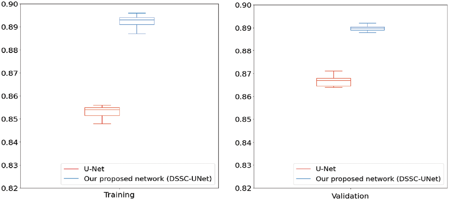
Figure 7: Box plot results of mean intersection over union (Mean-IoU) measured in training and validation

a: Fig. 8 below shows predicted segment images and ground truths for comparing U-Net and DSSC-UNet.

In addition, this paper compared the parameters between U-Net and DSSC-Unet. In the case of U-Net, the number of parameters is 13,304,371. DSSC-Unet is 18,156,275. This paper confirmed this difference occurred by the down-sampling in DSSC-Unet. The reason is that the output filter of down-sampling is twice as large as the input filter. As a result, the number of parameters in DSSC-Unet increased.

Figure 8: Results of compared input image’s ground truth with U-Net’s prediction and our proposed model (DSSC-UNet)’s prediction. Black labels in ground truth are ignored in prediction of U-Net and DSSC-UNet. The area surrounded by the red box is the extended area in Fig. 9

Figure 9: This is the result of expanding specific areas in input image’s ground truth, U-Net’s prediction, and our proposed model (DSSC-UNet)’s prediction. Compared to ground truth, DSSC-UNet captured more detail features and small objects from image than U-Net

To see whether the performance of the DSSC-UNet algorithm is significant, this paper conducted the normality test. The result is significant. (In the case of U-Net, the Shapiro-Wilk test’s P-value was 7.9053e-5 in training and 0.0007 in validation. In the case of our proposed network was 0.0011 in training and 3.1637e-5 in validation. Those are less than 0.05.) So, neither U-Net nor our proposed model follows the normal distribution. And the result of the Mann–Whitney U test is significant (P-value was 1.5252e-6 in training and 1.3940e-6 in validation.).

As a result, DSSC-UNet used more latent information for training by replacing max pooling with down-sampling. This approach was able to train more detailed information from feature maps and better classify small objects from images. In addition, the transposed convolution was replaced with the subpixel convolution in the expansive path. It expanded the feature maps as close as original with minimized loss of detailed information. Because diagonal elements of the original feature maps were used as additional information for summarized feature maps expansion. The reason for these, DSSC-UNet achieved higher segmentation accuracy than U-Net.

5  Conclusion

This paper proposed the method using down-sampling and subpixel convolution to improve accuracy in semantic segmentation. Our proposed model (DSSC-UNet) minimized the detailed context loss of the image when it reduced the size of the feature maps. And it preserved localization and detailed context during the expansion. As a result, this paper confirmed that DSSC-UNet showed higher accuracy than U-Net in semantic segmentation. In the future, it will apply DSSC-UNet to other datasets and utilize it in our previous resolution research [17]. In addition, various experiments will be conducted to maintain accuracy while reducing the increased parameters using 4 feature maps of down-sampling.

Funding Statement: The authors received no funding for this study.

Conflicts of Interest: The authors declare that they have no conflicts of interest to report regarding the present study.

References

1. S. Minaee, Y. Y. Boykov, F. Porikli, A. J. Plaza, N. Kehtarnavaz et al., “Image segmentation using deep learning: A survey,” IEEE Transactions on Pattern Analysis and Machine Intelligence, vol. 44, no. 7, pp. 3523–3542, 2021. [Google Scholar]
2. L. -C. Chen, G. Papandreou, I. Kokkinos, K. Murphy and A. L. Yuille, “Semantic image segmentation with deep convolutional nets and fully connected CRFs,” arXiv:1412.7062, 2014. [Online]. Available: http://arxiv.org/abs/1412.7062. [Google Scholar]
3. K. Sun, Y. Zhao, B. Jiang, T. Cheng, B. Xiao et al., “High-resolution representations for labeling pixels and regions,” arXiv:1904.04514, 2019. [Online]. Available: http://arxiv.org/abs/1904.04514. [Google Scholar]
4. H. Zhao, J. Shi, X. Qi, X. Wang and J. Jia, “Pyramid scene parsing network,” in Proc. of the IEEE Conf. on Computer Vision and Pattern Recognition, Honolulu, HI, USA, pp. 6230–6239, 2017. [Google Scholar]
5. A. Krizhevsky, I. Sutskever and G. E. Hinton, “Imagenet classification with deep convolutional neural networks,” Advances in Neural Information Processing Systems, vol. 1, pp. 1097–1105, 2012. [Google Scholar]
6. K. Simonyan and A. Zisserman, “Very deep convolutional networks for large-scale image recognition,” arXiv:1409.1556, 2014. [Online]. Available: http://arxiv.org/abs/1409.1556. [Google Scholar]
7. C. Szegedy, W. Liu, Y. Jia, P. Sermanet, S. Reed et al., “Going deeper with convolutions,” in Proc. of the IEEE Conf. on Computer Vision and Pattern Recognition, Boston, MA, USA, pp. 1–9, 2015. [Google Scholar]
8. J. Long, E. Shelhamer and T. Darrell, “Fully convolutional networks for semantic segmentation,” in Proc. of the IEEE Conf. on Computer Vision and Pattern Recognition, Boston, MA, USA, pp. 3431–3440, 2015. [Google Scholar]
9. O. Ronneberger, P. Fischer and T. Brox, “U-Net: Convolutional networks for biomedical image segmentation,” in Int. Conf. on Medical Image Computing and Computer-Assisted Intervention, Munich, Germany, vol. 9531, pp. 234–241, 2015. [Google Scholar]
10. V. Badrinarayanan, A. Kendall and R. Cipolla, “SegNet: A deep convolutional encoder-decoder architecture for image segmentation,” IEEE Transactions on Pattern Analysis and Machine Intelligence, vol. 39, no. 12, pp. 2481–2495, 2017. [Google Scholar]
11. B. Shuai, T. Liu and G. Wang, “Improving fully convolution network for semantic segmentation,” arXiv:1611.08986, 2016. [Online]. Available: http://arxiv.org/abs/1611.08986. [Google Scholar]
12. S. Shin, S. Lee and H. Han, “A study on residual U-net for semantic segmentation based on deep learning,” Journal of Digital Convergence, vol. 19, no. 6, pp. 251–258, 2021. [Google Scholar]
13. W. Shi, J. Caballero, F. Huszár, J. Totz, A. P. Aitken et al., “Real-time single image and video super-resolution using an efficient sub-pixel convolutional neural network,” in Proc. of the IEEE Conf. on Computer Vision and Pattern Recognition, Las Vegas, NV, USA, pp. 1874–1883, 2016. [Google Scholar]
14. W. Shi, J. Caballero, L. Theis, F. Huszar, A. P. Aitken et al., “Is the deconvolution layer the same as a convolutional layer?,” arXiv:1609.07009, 2016. [Online]. Available: http://arxiv.org/abs/1609.07009. [Google Scholar]
15. Y. Kinoshita and H. Kiya, “Fixed smooth convolutional layer for avoiding checkerboard artifacts in CNNS,” in ICASSP 2020–2020 IEEE Int. Conf. on Acoustics, Speech and Signal Processing (ICASSP), Barcelona, Spain, pp. 3712–3716, 2020. [Google Scholar]
16. M. Cordts, M. Omran, S. Ramos, T. Rehfeld, M. Enzweiler et al., “The cityscapes dataset for semantic urban scene understanding,” in Proc. of the IEEE Conf. on Computer Vision and Pattern Recognition, Las Vegas, NV, USA, pp. 3213–3223, 2016. [Google Scholar]
17. B. Shrestha, Y. M. Kwon, D. K. Chung and W. M. Gal, “The atrous cnn method with short computation time for super-resolution,” International Journal of Computing and Digital Systems, vol. 9, no. 2, pp. 221–227, 2020. [Google Scholar]
Cite This Article
Copyright © 2023 The Author(s). Published by Tech Science Press.
This work is licensed under a Creative Commons Attribution 4.0 International License , which permits unrestricted use, distribution, and reproduction in any medium, provided the original work is properly cited.
Downloads
Citation Tools