Automated Artificial Intelligence Empowered White Blood Cells Classification Model

1  Introduction

White blood cells (WBC), or leucocytes, acts as an important part in safeguarding the human from foreign invaders and dangerous diseases, which include bacteria and viruses. WBC is classified into 4 major types, such as lymphocytes, monocytes, neutrophils, and eosinophils and it is recognized by its operational and physical features [1]. WBC count is very significant in deciding the presence and diagnosis of diseases as such WBC subtype counts taken into consideration for the importance of the healthcare sector. Generally, such cell counts were conducted manually, but it could be applied in labs which do not have accessibility to anyone of the automated instruments [2]. During manual distinctive methodology, a diagnostician examines the blood samples through a microscope for determining the count and categorizes such leucocytes [3]. Automatic system predominantly utilize Coulter counting, cytochemical, and dynamic and static light scattering blood sample testing processes. In such process, the data will be examined and plotted for forming particular groups which relate to distinct leucocyte types [4,5]. But, whenever variant or abnormal WBCs were existing, such automated outcomes were probably mistaken, and therefore, the manual distinctive methodology was taken as a favorable choice in determination of the count and categorization of WBC. Leukemia arises because of huge quantity of WBCs in the immune system, that protects the platelets and red blood cells (RBCs) of blood which have to be healthy [6]. On the basis of developing speed and its impacts, physicians classify this into 4 types they are lymphocytic leukemia, acute leukemia, chronic leukemia, and myelogenous leukemia [7]. Leukemia is a disease that occurs in death. For overcoming the disease severity, it becomes essential to identify the shapes of immature cells in the primary stages which diminishes the death rate. Most of the researchers recommended distinct methods and systems for the detection, segmentation, and categorization of leukemia, and yet, there exist certain gaps in this field.

Commonly, the recognition needs a lab setting in which received images of blood cells were stained with the help of specialized chemicals (e.g., reagents), and then it is analyzed through a microscope by an expert [8]. But this procedure was very sensitive and needs a no or minimum analysis mistake by the expert. Unluckily, experts might be tired after numerous hours of check-ups and that results in erroneous recognition of the distinct WBC. Deep learning (DL) utilizing Convolution Neural Networks (CNN) is recently the finest option in medical imaging application areas like classification and detection [9]. CNNs attain the finest outcomes on huge data sets, it needs much more data and computational sources for training purposes. Sometimes the dataset is restricted and it is not adequate for training a CNN from scratch. In such cases, using the power of CNNs and reducing the computational costs, transfer learning (TL) could be utilized [10]. In this method, the CNN is primarily pretrained over a great and varied generic image datasets and implied to a particular task.

This paper introduces an Aquila Optimizer with Transfer Learning based Automated White Blood Cells Classification (AOTL-WBCC) technique. The presented AOTL-WBCC model executes data normalization and data augmentation process (rotation and zooming) at the initial stage. In addition, the residual network (ResNet) model was employed for feature extraction in which the initial hyperparameter values of the ResNet system are tuned by the use of AO algorithm. Finally, Bayesian neural network (BNN) classification methodology is implemented for the identification of WBC images into distinct classes. The experimental validation of the AOTL-WBCC method is performed with the help of Kaggle dataset.

2  Related Works

In [11], the authors illustrate WBC classification into 6 types such as eosinophils, lymphocytes, neutrophils, basophils, abnormal cells, and monocytes. The authors offer the comparability of DL methods and classical image processing techniques for WBC classification. Lu et al. [12] suggest a DL network known as WBC-Net, that references ResNet and UNet ++. In specific, WBC-Net devise a context aware feature encoder having residual blocks for extracting multi-scale structures, and launches mixed skip pathways over the dense convolutional blocks for acquiring and fusing image features at distinct scales. In addition to this, WBC-Net utilizes a decoder integrating deconvolution and convolution for refining the WBC segmentation mask. Also, WBC-Net describes a loss function on the basis of the Tversky index and cross-entropy for training the network.

In [13], the authors build a new CNN method termed as WBCNet system which is able to completely derive features of the microscopic WBC image through merging improved activation function, batch normalization algorithm, and residual convolution architecture. WBCNet system consists of 33 layers of network structure, whereof speed was highly enhanced than conventional CNN system at the time of training, and it could rapidly find the type of WBC images. Cheuque et al. [14] grant a 2-stage hybrid multi-level structure which effectively categorizes 4 cell groups they are segmented neutrophils, lymphocytes, eosinophils (polymorphonuclear), and monocytes (mononuclear). In the initial stage, a Faster region based CNN (R-CNN) network was implied for the recognition of the areas of interest of WBC, along with the division of mononuclear cell from polymorphonuclear cell. After the separation, 2 parallel CNNs with the MobileNet framework were utilized for identifying the subcategories in the next stage.

Dong et al. [15] suggest a WBC classification method which incorporates artificial and deep learning features. This methodology not just utilizes artificial features, since further complies the self-learning abilities of Inception V3 for making complete usage of the feature information of the image. Meanwhile, this article presents the TL algorithm for solving the issue of the dataset limits. Manthouri et al. [16] offer a deep neural network (DNN) for functioning of microscopic imageries of blood corpuscles. Processing such imageries become an important one as WBC and its features were utilized for diagnosing distinct diseases. In this study, the authors devise and apply a dependable processing system for blood samples and categorize 5 various kinds of WBC under microscopic imageries. The authors employ the Gram-Schmidt method for the purpose of segmentation. In order to classify different kinds of WBC, the authors merge deep CNN and Scale-Invariant Feature Transform (SIFT) feature recognition methods.

3  The Proposed Model

In this article, a novel AOTL-WBCC approach was advanced for the detection and classification of WBC. The presented AOTL-WBCC technique follows a sequence of processes namely pre-processing, data augmentation, ResNet50 related feature extraction, AO related hyperparameter optimization, and BNN related classification. Fig. 1 shows the overall process of AOTL-WBCC approach.

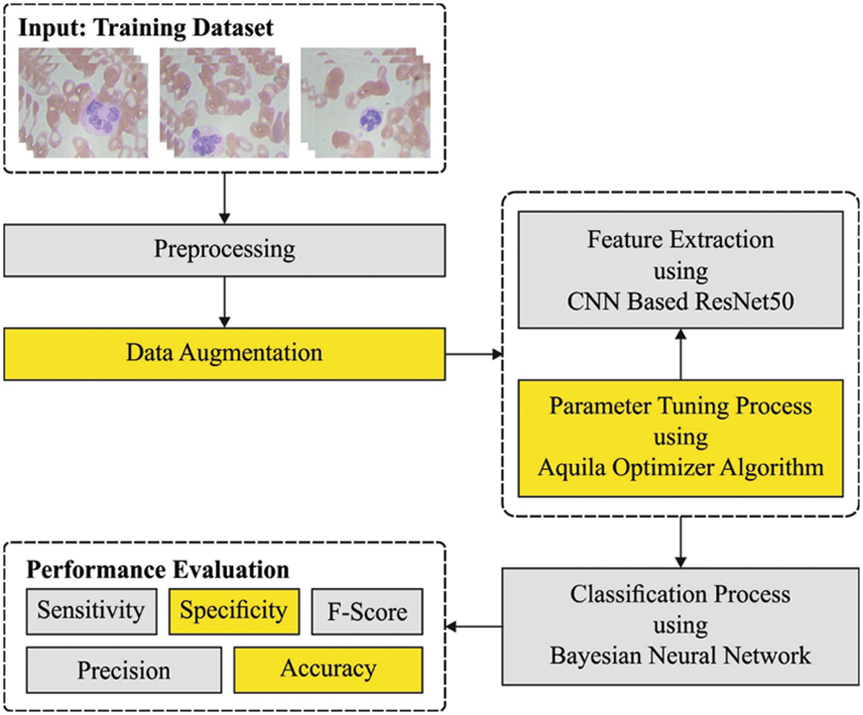
Figure 1: Overall process of AOTL-WBCC technique

3.1 Data Preprocessing

The data underwent a normalization pre-processing method to retain its arithmetical stability to DL model. At first, WBC image is in an RGB format with pixel values of 0 to 255. Through normalizing the input image, the DL model is quickly trained. To increase the efficacy of the DL models, a large set of data is needed. But accessing the dataset frequently comes with many constraints. Thus, to overcome the challenges, data augmentation technique is applied to rise the sample image count in the sample data. Data augmentation models like Rotation and Zooming are employed. The rotation data augmentation method is executed in a clockwise direction with an angle of 90 degree. Also, zooming augmentation method is implemented on image data by taking the 0.5 and 0.8 zooming factor values. To over the imbalance problem, the abovementioned data augmentation technique is implemented. After using the data augmentation technique, the sample data in every class was improved.

3.2 Feature Extraction: ResNet50 Model

Next to data pre-processing, the ResNet50 model is utilized for feature extraction. It is a deep convolution network where the underlying concept is to avoid blocking of convolution layer with the aid of shortcut connection [17]. The elementary block known as “bottleneck” block follows two basic rules one is for a similar output feature map size, the layer has a similar amount of filter and another one is when the feature map size can be halved, the filter count is doubled. The down-sampling can be straightly implemented by convolution layer that has a stride of 2 and BN can be implemented before rectified linear unit (ReLU) activation and immediately after every convolution. Once the output and input are of a similar dimension, the identity shortcut is utilized. Once the dimension increases, the presented shortcut is utilized for matching dimensions via 1 × 1 convolution. In both scenarios, once shortcut goes across feature map of 2 sizes, they can be implemented with a stride of 2.

With transfer learning technique, we transported the initial forty-nine layers of ResNet-50 that may left frozen on the WBC classification method. This layer is viewed as learned feature extraction layer. The activation map produced via learned feature extraction layer is generally known as bottleneck feature. With the bottleneck feature of WBC image as input, we trained a twenty-five FC softmax layer, because we have twenty-five classes, and later replaces the 1,000 FC softmax layers by the trainable twenty-five FC softmax layers.

3.3 Hyperparameter Optimization

In this study, the initial hyperparameter values of the ResN et algorithm are tuned by the use of AO algorithm [18,19]. AO is a population based algorithm, the prominent rules initiates by the population of candidate solution (X) as follows, stochastically created between the lower boundary (LB) and upper boundary (UB) of the given problem [20]. An optimal solution attained in each iteration is determined by the following matrix

x=[x1,1⋯x1,jx1,Dim−1x1,Dimx2,1⋯x2,j⋯x2,Dim⋯⋯xi,j⋯⋯⋮⋮⋮⋮⋮xN−1,1⋯xN−1,j⋯xN−1,DimxN,1⋯xN,jxN,Dim−1xN,Dim](1)

In Eq. (1) X denotes the set of existing candidate solutions that are arbitrarily created by the following equation, Xi denotes the decision value of ith solution, N refers to the overall number of candidate solutions (population), and Dim stands for the dimension problem.

Xij=rand×(UBj−LBj)+LBj,i=1,2,…..,Nj=1,2,…,Dim(2)

In Eq. (2), the arbitrary number can be represented as rand, the jth lower bound is denoted byLBj, and the jth upper bound is characterized by UBj. The AO algorithm was transmitting in exploration to exploitation phases using discrete performance based on the term when t≤(23)∗T the exploration stage is implemented; otherwise, the exploitation stage is carried out. Here, the AO enormously explorer in great soar to determine the searching region. In the following, the mathematical expression of the given problem is demonstrated.

X1(t+1)=Xbest(t)×(1−tT)+(XM(t)−Xbest(t)∗rand)(3)

In Eq. (3), the solution of subsequent round of t is represented as X1(t+1) that is generated by primary search model (X1). Xbest(t) indicates the optimal solution attained until tth iteration, this regenerates the assessed prey location. The equation (1−tT) is used for controlling the extended search (exploration) with the iteration count. XM(t) determines the place mean value of existing solution related at tth iteration viz. calculated using the following equation. The arbitrary value ranges from [0, 1] is indicated as rand. r and T correspondingly demonstrate the current and the maximal rounds.

XM(t)=1N∑i=1NXj(t),∀j=1,2,…,Dim(4)

In Eq. (4). The dimensional size of the problem can be represented by the term Dim and the population size is represented by the term N. Fig. 2 depicts the flowchart of AO algorithm.

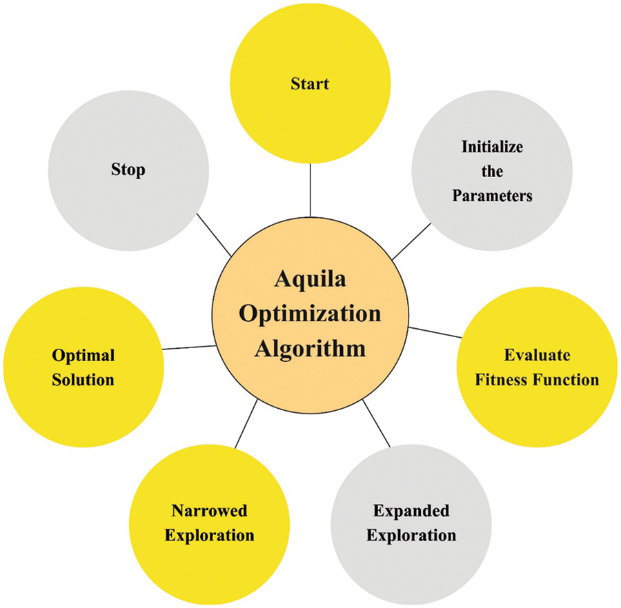
Figure 2: Flowchart of AO algorithm

If the prey position was begin in a great soar, the Aquila circle over the target, places the land, and subsequent attack, during the next searching technique(X2). The mathematical expression can be represented as follows.

X2(t+1)=Xbest(t)×Levy(D)+XR(t)+(y−x)∗rand(5)

In Eq. (5), X2(t+1) indicates the solution of following iteration of r which can be generated through the second technique (X2). D denotes the dimensional space, and Levy(D) denotes the levy flight distribution function that is calculated by the following equation. XR(t) refers to the arbitrarily attained solution from the interval of 1[N] at ith iterations.

Levy(D)=s×u×σ|v|1β(6)

In Eq. (6), s denotes the constant value is fixed as 0.01, u and v indicates the arbitrary number lies within [0, 1]. σ can be evaluated by the following expression.

σ=(Γ(1+β)×sine(πβ2)Γ(1+β2)×β×2(β−12))(7)

In Eq. (5), y and x are applied to provide the spiral shape in the search technique is evaluated by:

y=r×cos(θ)(8)

x=r×sin(θ)(9)

where,

r=r1+U×D1(10)

θ=−ω×D1+θ1(11)

θ1=3×π2(12)

r1 get the value within the range of [1–20] to set the number of searching cycles, U represents the less value fixed as 0.00565. D1 determines the integer number in 1 to the length of searching space(Dim), and ω refers to the lesser value fixed as 0.005. Here, the AO makes use of the preferred area of the target to get the nearby prey, and attack is arithmetically expressed by using subsequent formula.

X3(t+1)=(Xbest(t)−XM(t))×α−rand+((UB−LB)×rand+LB)×δ(13)

In Eq. (12), the solution of succeeding round of r implies the expression X3(r+1) specifically generated by 3rd search technique (X3). Xbest(t) denotes the evaluated position of prey until ith iteration (the optimal obtained solution), and XM(t) signifies the mean value of existing solution at rth iteration that is calculated. rand indicates the arbitrary integer lies within [0, 1]. In the fourth manner (X4), the Aquila turn out to be near the prey, the Aquila attacks the prey on the land according to stochastic movement and it is formulated by using the succeeding equation

X4(t+1)=QF×Xbest(t)−(G1×X(t)×rand)−G2×Levy(D)+rand×G1(14)

In Eq. (14), X4(t+1) denotes the solution of following t iteration that has been produced by the fourth manner (X4). QF illustrates the quality function applied to equilibrium the searching process that is calculated.

According to this article, the reduction of the classifier error rate was regarded as the fitness function, as provided in Eq. (15). The optimum resolution contains minimum error rates and the poor resolution reaches a higher error rates.

fitness(xi)=Classifier Error Rate(xi)

=number of misclassified WBC imagesTotal number of WBC images∗100(15)

3.4 WBC Classification

Finally, the BNN classification algorithm can be implied for the identification of WBC images into distinct classes. It provides a probabilistic interpretation of DL model by positioning distribution over the neural network weight [21]. Assume that trained data D={x,y} with input x={x1,…,xN} and respective output y={y1,…,yN}, in parametric Bayesian settings, we would like to infer a distribution over w weight as a function y=fw(x) which indicates the neural network (NN) mechanism. A previous distribution is allocated over the p(w) weights that capture previous beliefs where the parameter has generated the output beforehand observing any dataset. Assume that the evidence dataset p(y|x), previous model, and distribution likelihood p(y|x,w), the goal is inferring the latter distribution over the p(w|D) weights:

p(w|D)=p(y|x,w)p(w)∫p(y|x,w)p(w)dw(16)

Compute the latter distribution p(w|D) is frequently intractable, few presented techniques accomplish an analytically tractable inference including expectation propagation, variational inference, Markov Chain Monte Carlo (MCMC) sampling related probabilistic inference, Monte Carlo dropout and approximate inference. Prediction distribution can be attained by more than one stochastic forward pass on the network while sampling from the weight posterior through Monte Carlo estimator. Eq. (17) illustrates the prediction distribution of output y∗ assumed new input x∗:

p(y∗|x∗,D)=∫p(y∗|x∗,w)p(w|D)dw

p(y∗|x∗,D)≈1T∑i=1Tp(y∗|x∗,wi),wi∼p(w|D)(17)

In Eq. (17), number of Monte Carlo samples can be represented as T.

4  Performance Validation

The experimental validation of the AOTL-WBCC methodology can be tested with the use of the blood cell images from the Kaggle dataset (available at https://www.kaggle.com/datasets/paultimothymooney/blood-cells). It includes four classes and the details regards to the dataset are shown in Table 1. Some sample images are displayed in Fig. 3.

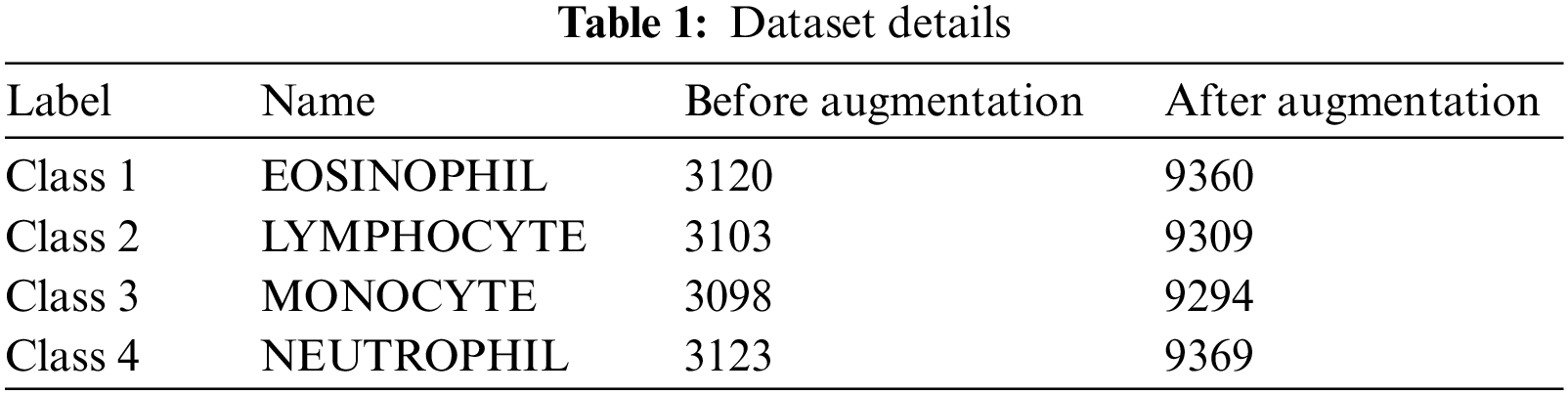
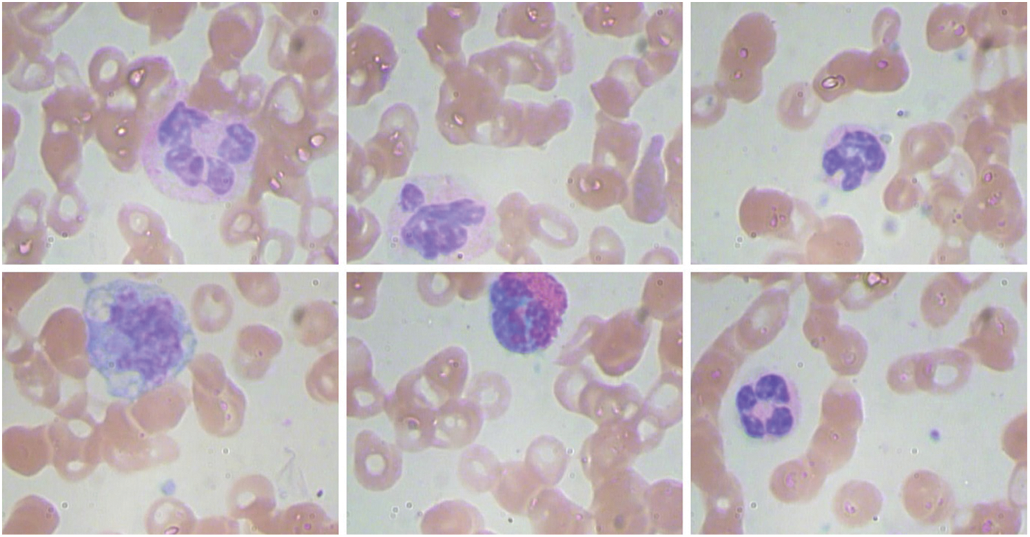
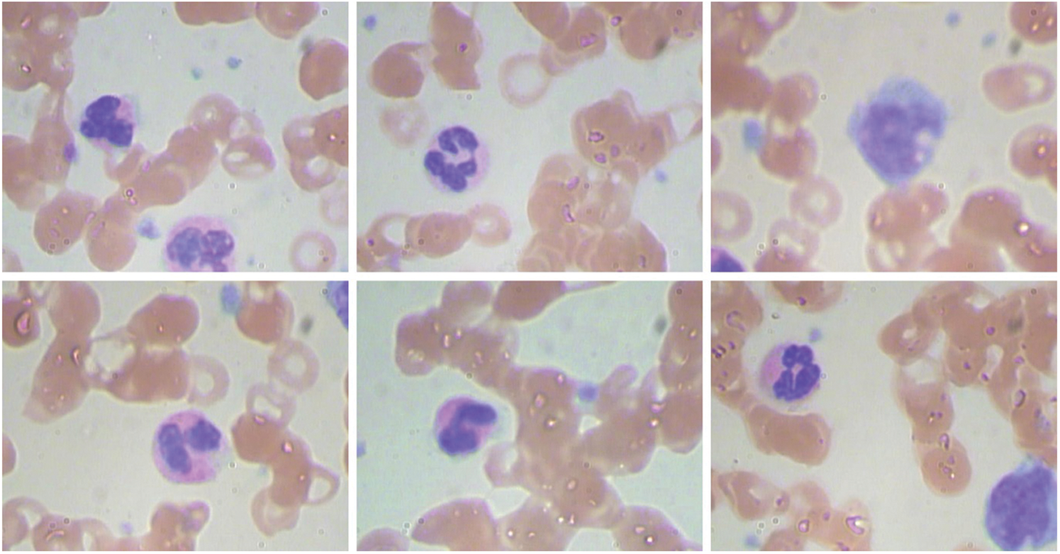
Figure 3: Sample images

Fig. 4 demonstrates a clear set of confusion matrices generated by the AOTL-WBCC model on varying sizes of training (TR) and testing (TS) data. The figure pointed out that the AOTL-WBCC model has shown effectual identification of WBC classes under all aspects.

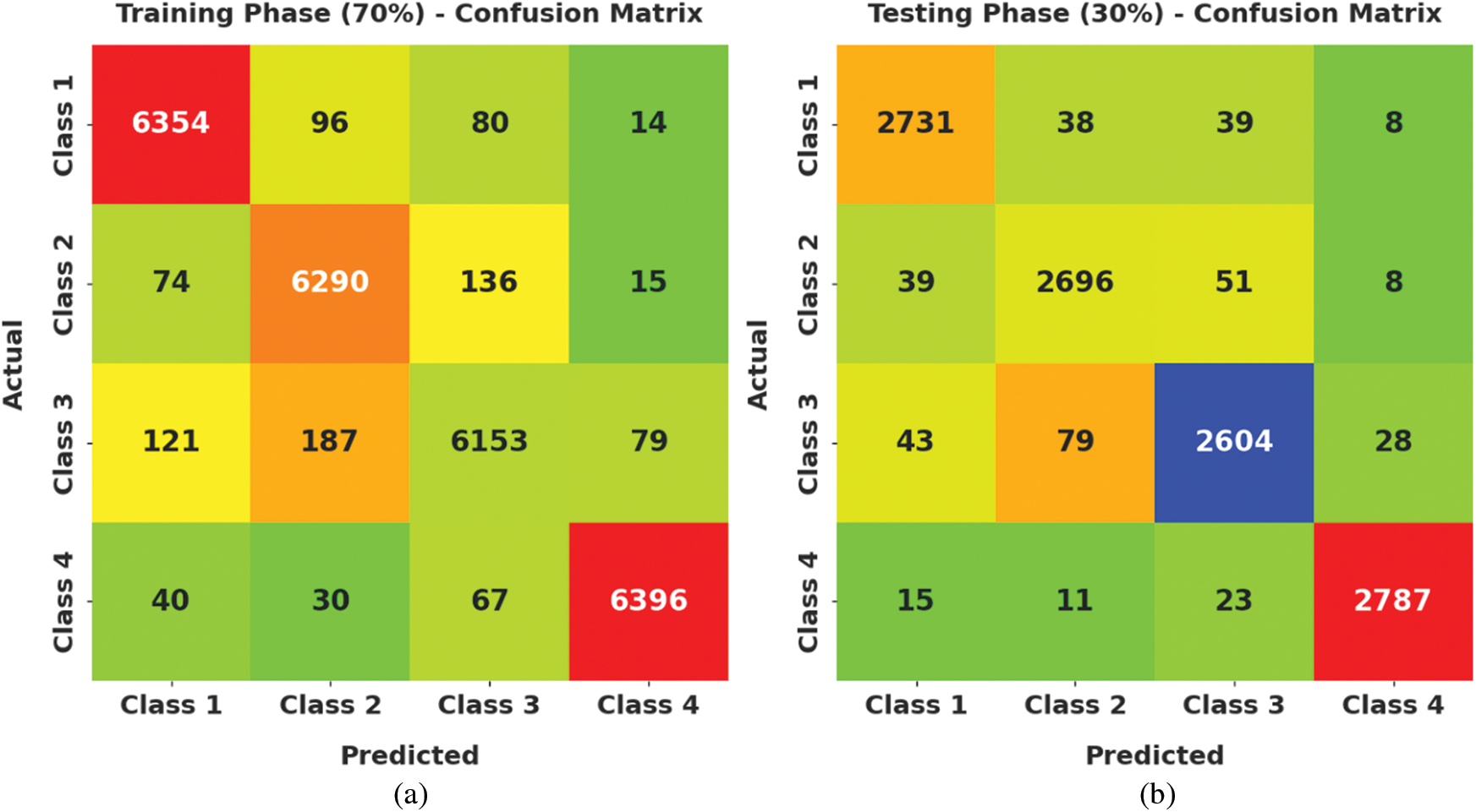
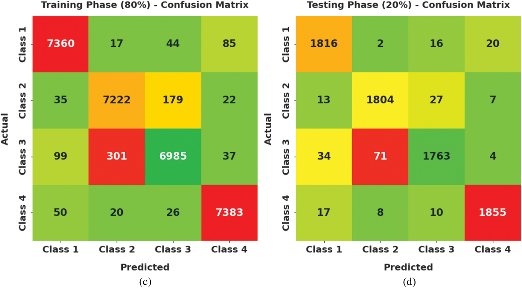
Figure 4: Confusion matrices of AOTL-WBCC technique (a) 70% of TR data, (b) 30% of TS data, (c) 80% of TR data, and (d) 20% of TS data

Table 2 provides an overall WBC classification results of the AOTL-WBCC model on 70% of TR and 30% of TS data. Fig. 5 reports the result analysis of the AOTL-WBCC model on 70% of TR data. The figure implied that the AOTL-WBCC model has offered enhanced outcomes in the classification of each WBC class. For instance, the AOTL-WBCC model has recognized class 1 samples with accuy, precn, sensy, specy, and Fscore of 98.37%, 96.43%, 97.10%, 98.80%, and 96.76% respectively. In addition, the AOTL-WBCC approach has recognized class 3 samples with accuy, precn, sensy, specy, and Fscore of 97.44%, 95.60%, 94.08%, 98.56%, and 94.84% correspondingly. Also, the AOTL-WBCC algorithm has recognized class 4 samples with accuy, precn, sensy, specy, and Fscore of 99.06%, 98.34%, 97.90%, 99.45%, and 98.12% correspondingly.

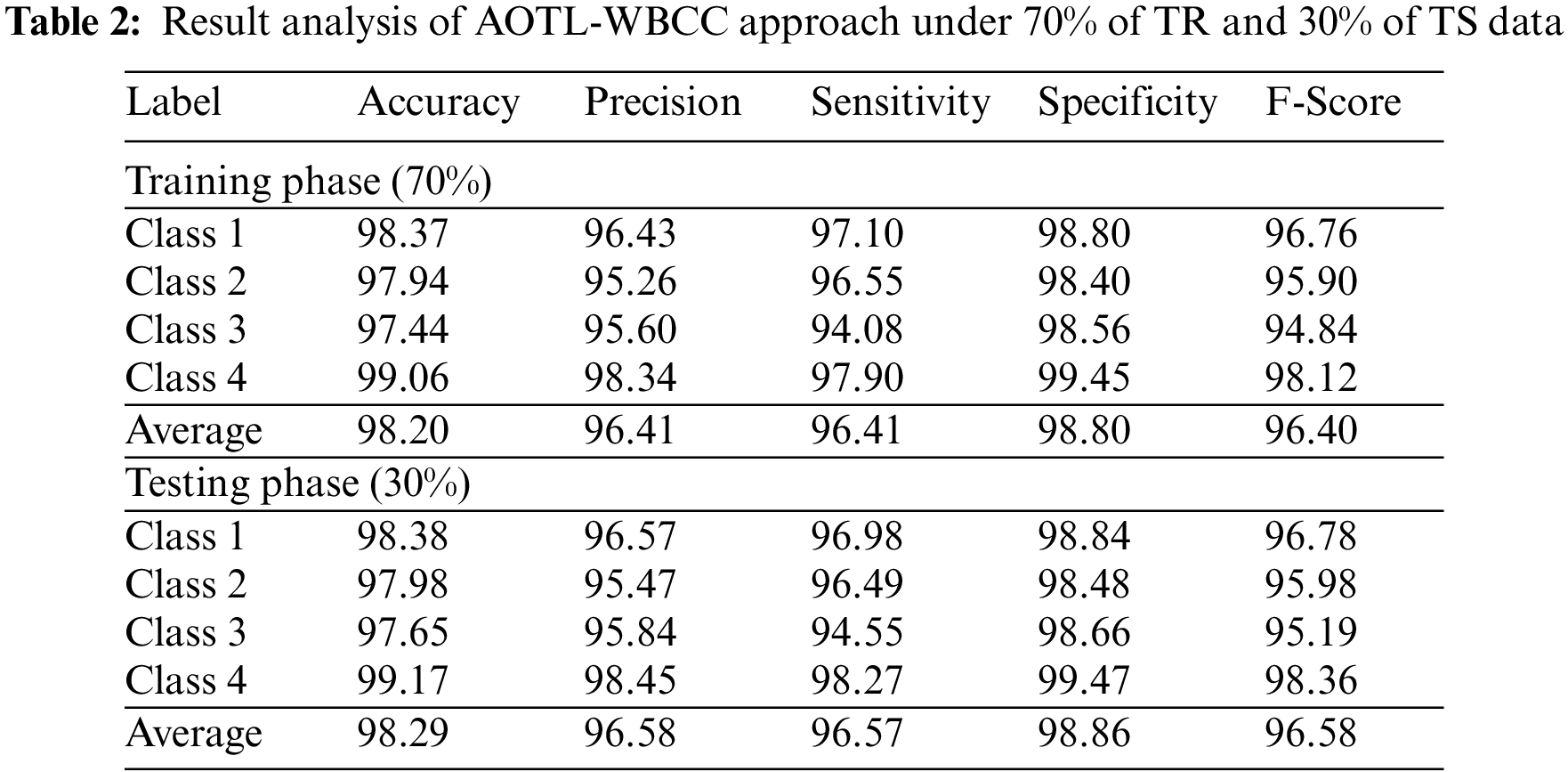
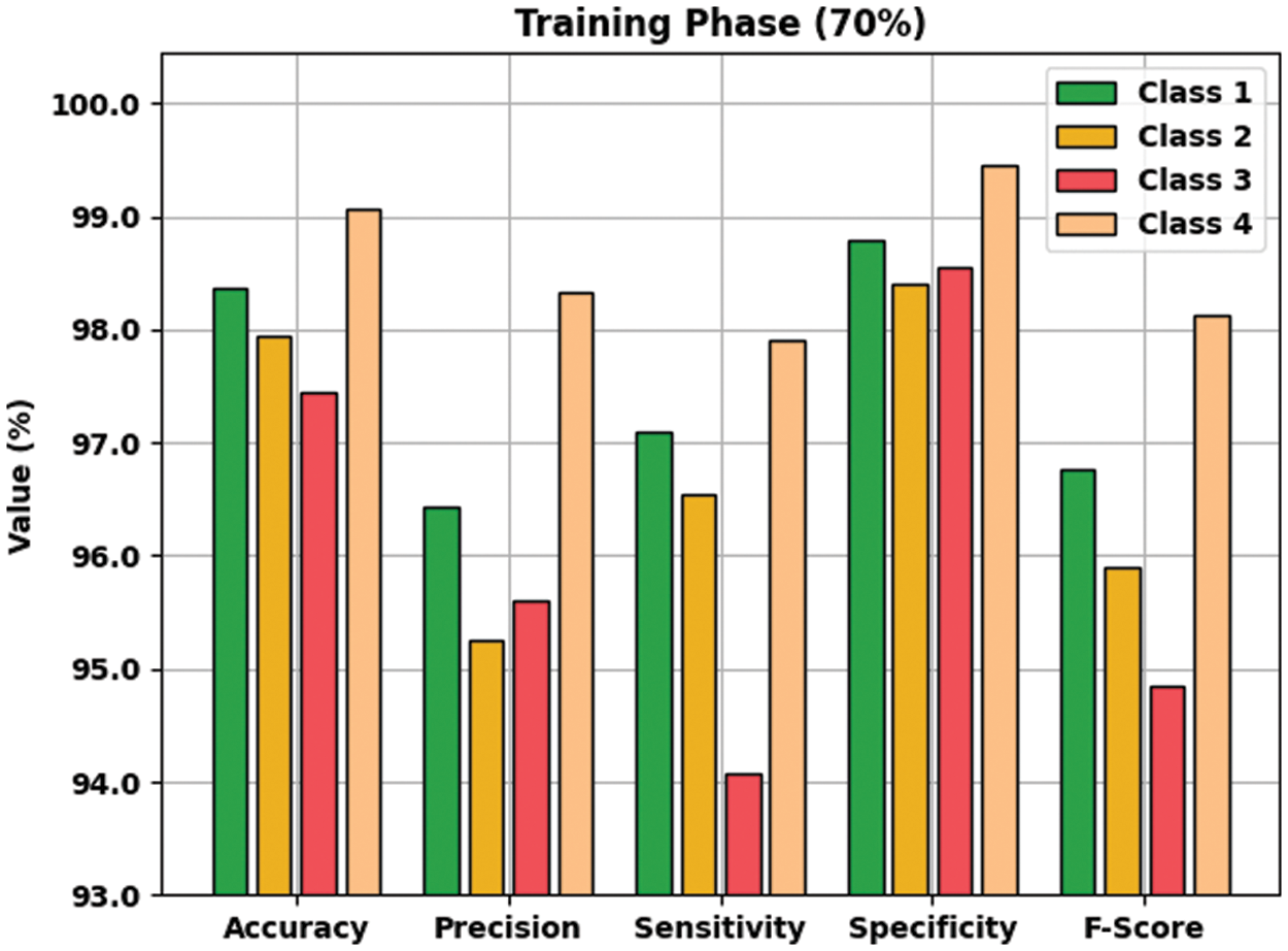
Figure 5: Result analysis of AOTL-WBCC algorithm under 70% of TR data

Fig. 6 defines the result analysis of the AOTL-WBCC methodology on 30% of TS data. The figure exposed the AOTL-WBCC methodology has obtainable higher outcome on the classification of each WBC class. For instance, the AOTL-WBCC algorithm has recognized class 1 samples with accuy, precn, sensy, specy, and Fscore of 98.38%, 96.57%, 96.98%, 98.84%, and 96.78% correspondingly. Likewise, the AOTL-WBCC model has recognized class 3 samples with accuy, precn, sensy, specy, and Fscore of 97.65%, 95.84%, 94.55%, 98.66%, and 95.19% correspondingly. Eventually, the AOTL-WBCC algorithm has recognized class 4 samples with accuy, precn, sensy, specy, and Fscore of 99.17%, 98.45%, 98.27%, 99.47%, and 98.36% respectively.

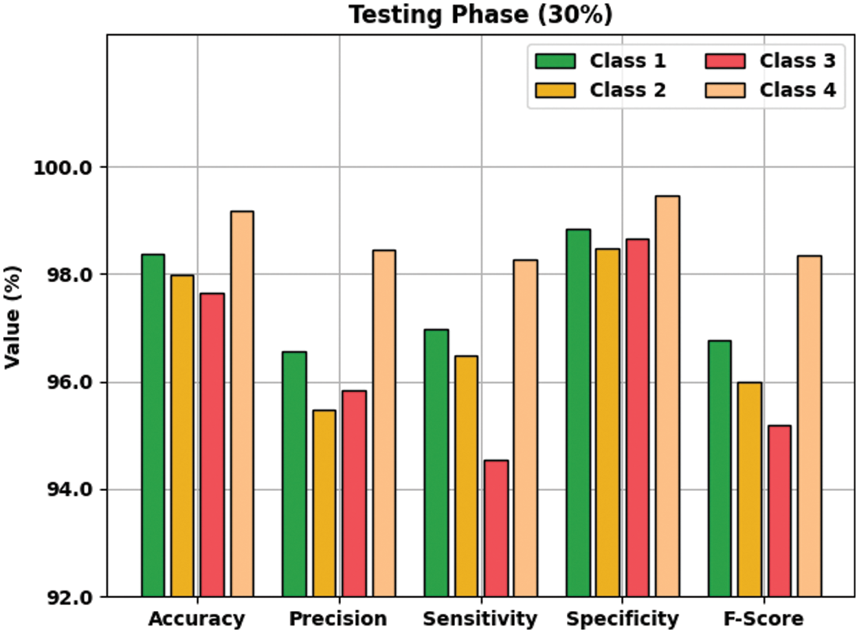
Figure 6: Result analysis of AOTL-WBCC algorithm under 30% of TS data

Tab. 3 offers an overall WBC classification outcome of the AOTL-WBCC methodology on 80% of TR and 20% of TS data. Fig. 7 reports the result analysis of the AOTL-WBCC approach on 80% of TR data. The figure exposed the AOTL-WBCC approach contains obtainable enhanced results on the classification of each WBC class. For sample, the AOTL-WBCC model has recognized class 1 samples with accuy, precn, sensy, specy, and Fscore of 98.90%, 97.56%, 98.05%, 99.18%, and 97.81% correspondingly. Followed, the AOTL-WBCC algorithm has recognized class 3 samples with accuy, precn, sensy, specy, and Fscore of 97.70%, 96.56%, 94.11%, 98.89%, and 95.32% respectively. At last, the AOTL-WBCC system has recognized class 4 samples with accuy, precn, sensy, specy, and Fscore of 99.20%, 98.09%, 98.72%, 99.36%, and 98.40% respectively.

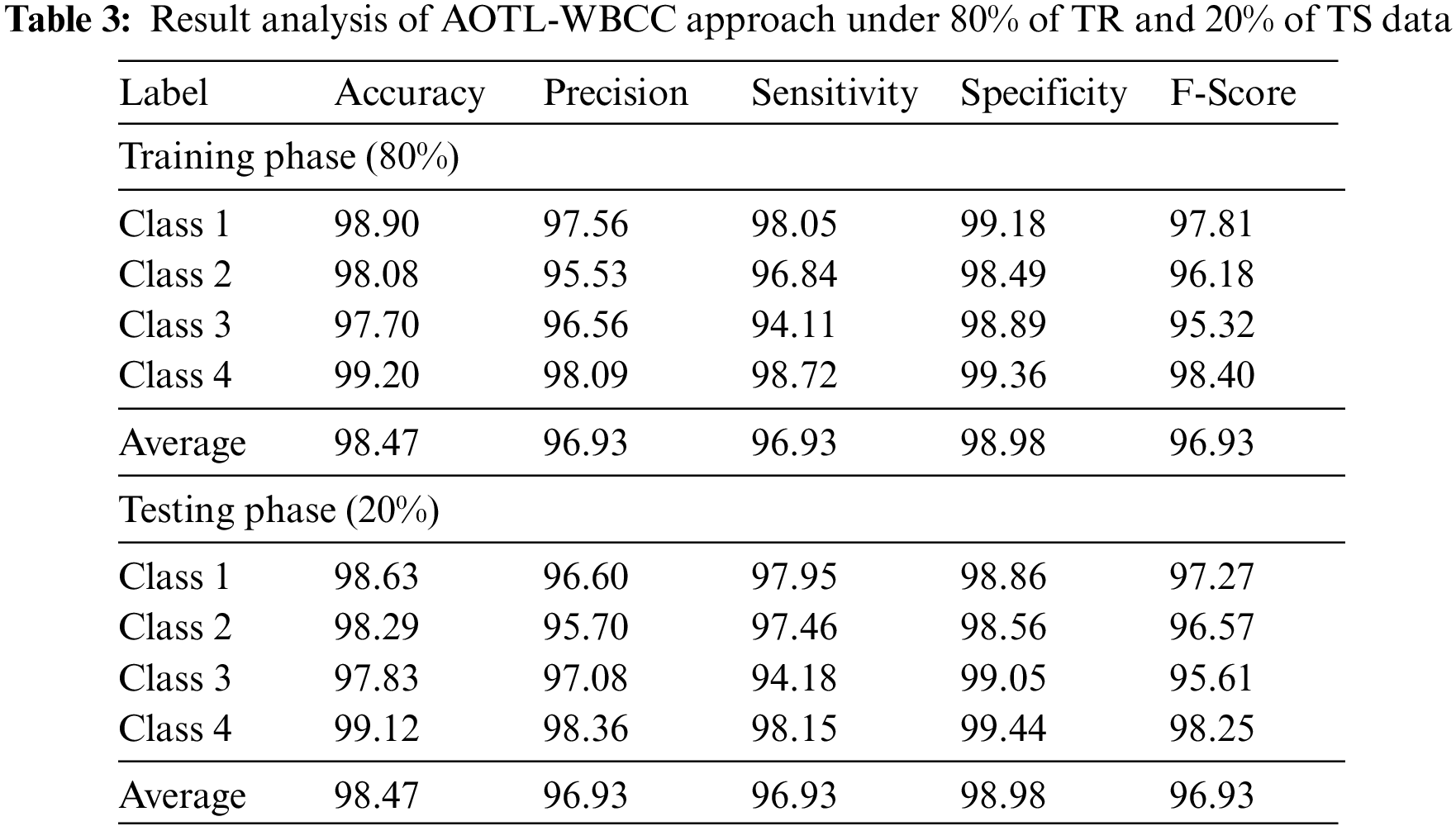
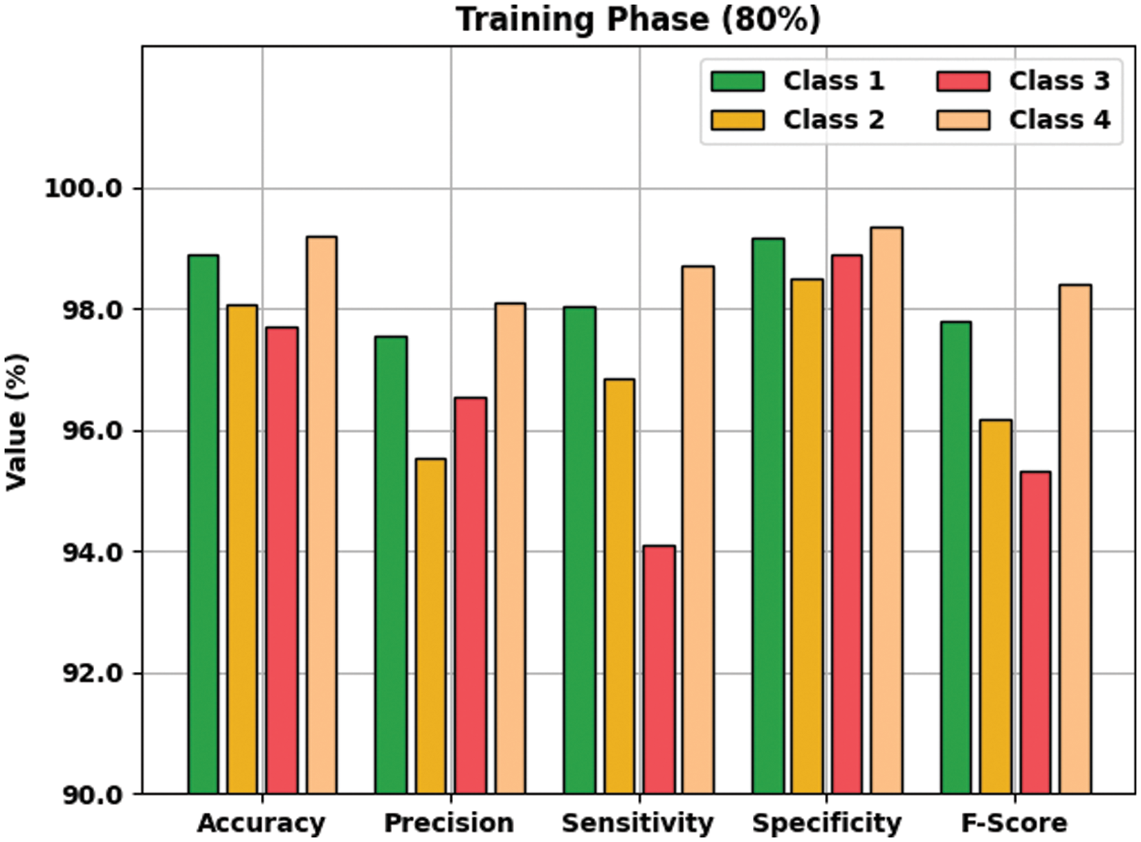
Figure 7: Result analysis of AOTL-WBCC algorithm under 80% of TR data

Fig. 8 demonstrates the result analysis of the AOTL-WBCC system on 20% of TS data. The figure implied that the AOTL-WBCC model has accessible improved outcomes on the classification of each WBC class. For instance, the AOTL-WBCC method has recognized class 1 samples with accuy, precn, sensy, specy, and Fscore of 98.63%, 96.60%, 97.95%, 98.86%, and 97.27% respectively. Similarly, the AOTL-WBCC model has recognized class 3 samples with accuy, precn, sensy, specy, and Fscore of 97.83%, 97.08%, 94.18%, 99.05%, and 95.61% correspondingly. Finally, the AOTL-WBCC algorithm has recognized class 4 samples with accuy, precn, sensy, specy, and Fscore of 99.12%, 98.36%, 98.15%, 99.44%, and 98.25% correspondingly.

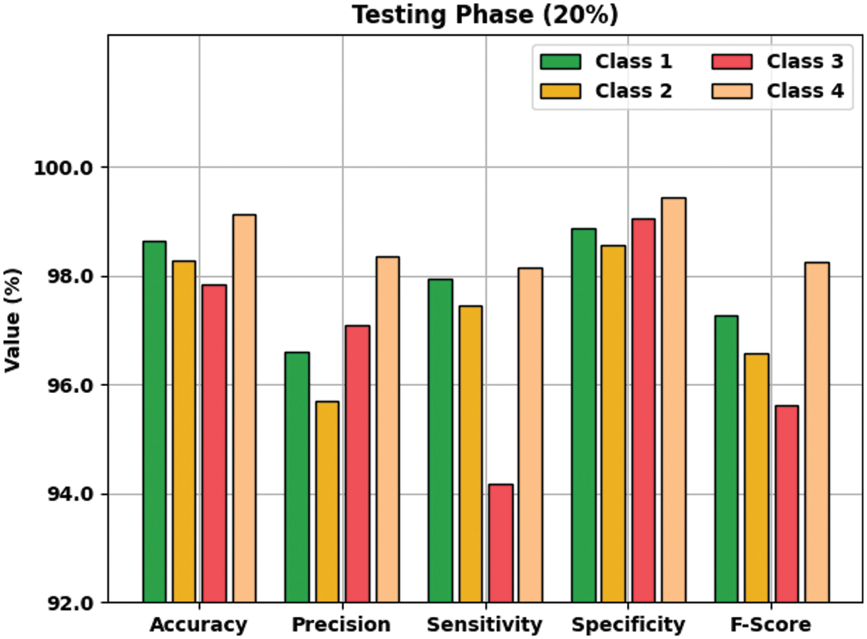
Figure 8: Result analysis of AOTL-WBCC algorithm under 20% of TS data

The training accuracy (TA) and validation accuracy (VA) attained by the AOTL-WBCC approach on test dataset is illustrated in Fig. 9. The experimental outcome implied that the AOTL-WBCC approach has gained maximum values of TA and VA. In specific, the VA seemed to be higher than TA. The training loss (TL) and validation loss (VL) achieved by the AOTL-WBCC system on test dataset are established in Fig. 10. The experimental outcome inferred that the AOTL-WBCC methodology has accomplished least values of TL and VL. In specific, the VL seemed that lower than TL.

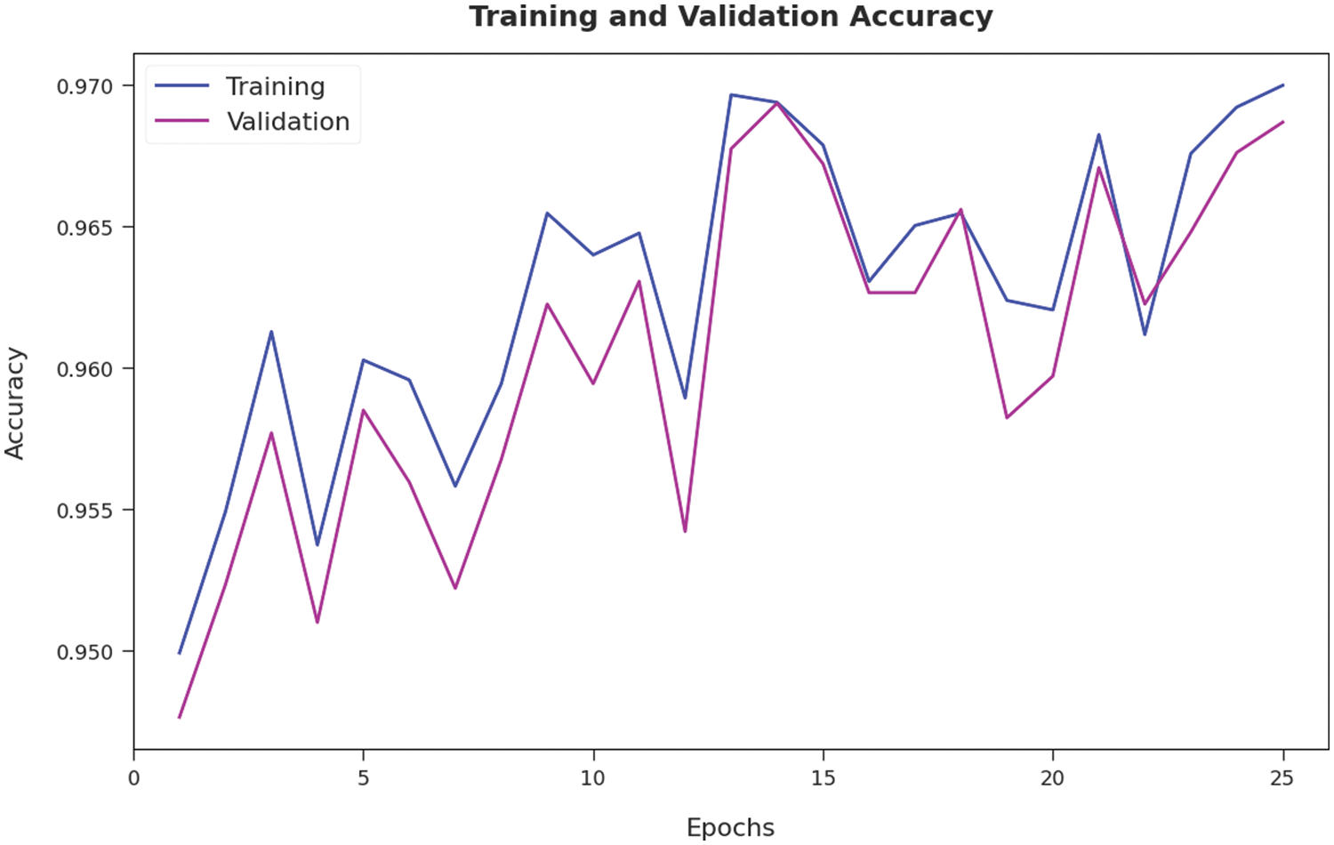
Figure 9: TA and VA analysis of AOTL-WBCC algorithm

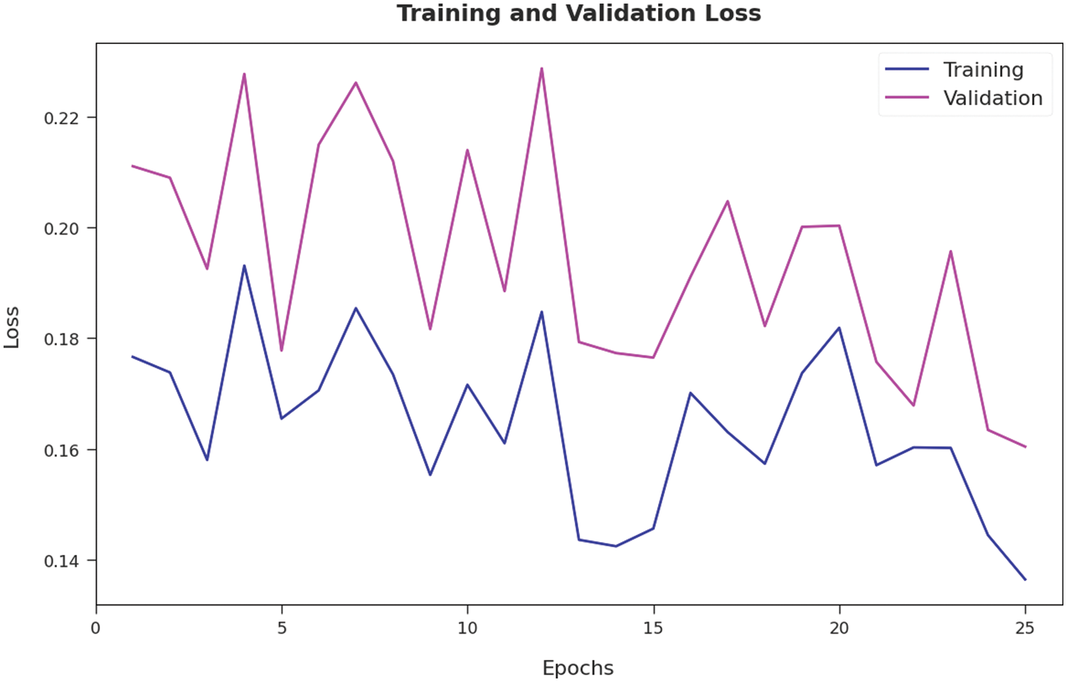
Figure 10: TL and VL analysis of AOTL-WBCC algorithm

A brief precision-recall examination of the AOTL-WBCC methodology on test dataset is portrayed in Fig. 11. By observing the figure, it can be noticed that the AOTL-WBCC model has accomplished maximal precision-recall performance under all classes.

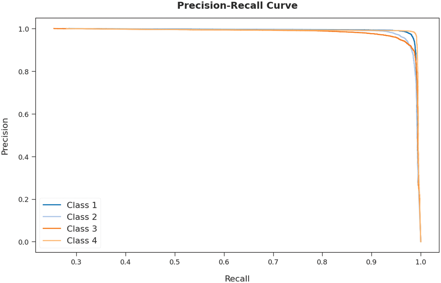
Figure 11: Precision-recall curve analysis of AOTL-WBCC algorithm

A detailed receiver operating characteristic (ROC) examination of the AOTL-WBCC system on test dataset is portrayed in Fig. 12. The results exposed the AOTL-WBCC algorithm has exhibited its ability in categorizing four different classes 1–4 on test dataset.

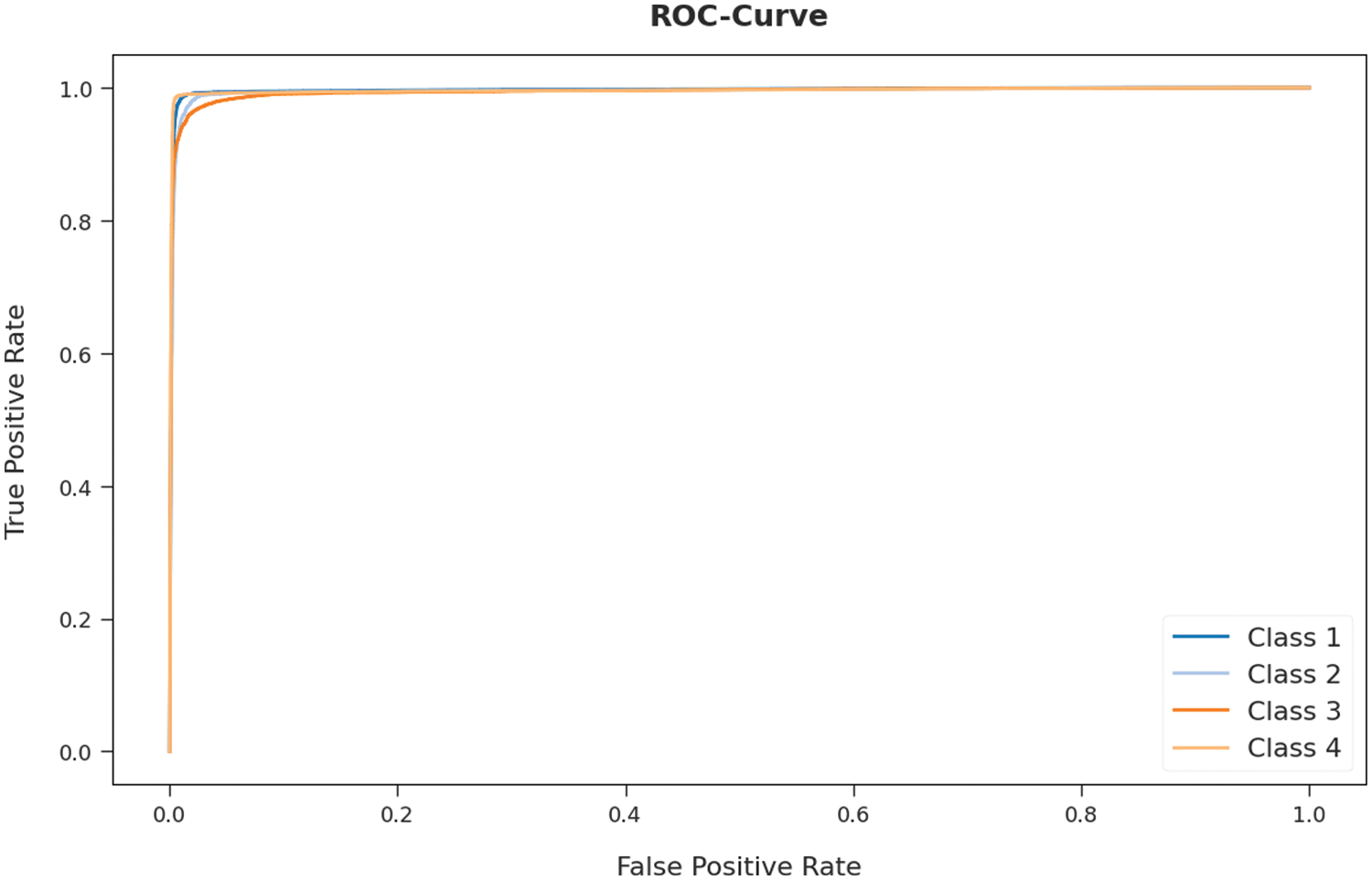
Figure 12: ROC curve analysis of AOTL-WBCC algorithm

Tab. 4 reports a brief comparison study of the AOTL-WBCC model with recent models. The figure indicated the DenseNet121 and Inceptionv3 models have attained minimal accuy of 93.19% and 91.39% respectively.

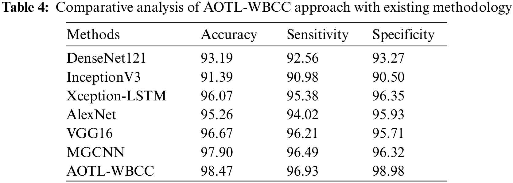
Followed by, the Xception-LSTM, AlexNet, and VGG16 models have obtained moderately closer accuy of 96.07%, 95.26%, and 96.67% respectively. Moreover, the multi-graph CNN (MGCNN) model has accomplished reasonable accuy of 97.90%. But, the presented AOTL-WBCC methodology has shown superior results with maximum accuy of 98.47%.

5  Conclusion

In this article, a novel AOTL-WBCC approach was enhanced for the classification and detection of WBC. The presented AOTL-WBCC system follows a sequence of processes namely pre-processing, data augmentation, ResNet50 related feature extraction, AO related hyperparameter optimization, and BNN related classification. In this case, the initial hyperparameter values of the ResN et algorithm are tuned by the use of AO algorithm. At last, the BNN classification algorithm has been implemented for the identification of WBC images into distinct classes. The experimental validation of the AOTL-WBCC model is performed using Kaggle dataset. The experimental results found that the AOTL-WBCC model has outperformed other techniques which are based on image processing and manual feature engineering approaches under different dimensions.

Funding Statement: The Deanship of Scientific Research (DSR) at King Abdulaziz University (KAU), Jeddah, Saudi Arabia has funded this project, under Grant No. KEP-1–120–42.

Conflicts of Interest: The authors declare that they have no conflicts of interest to report regarding the present study.

References

1. M. H. Motlagh, M. Jannesari, Z. Rezaei, M. Totonchi and H. Baharvand, “Automatic white blood cell classification using pre-trained deep learning models: ResNet and inception,” in Tenth Int. Conf. on Machine Vision (ICMV 2017), Vienna, Austria, pp. 105, 2018. [Google Scholar]
2. M. Yildirim and A. Çinar, “Classification of white blood cells by deep learning methods for diagnosing disease,” Revue D’Intelligence Artificielle, vol. 33, no. 5, pp. 335–340, 2019. [Google Scholar]
3. E. H. Mohamed, W. H. El-Behaidy, G. Khoriba and J. Li, “Improved white blood cells classification based on pre-trained deep learning models,” Journal of Communications Software and Systems, vol. 16, no. 1, pp. 37–45, 2020. [Google Scholar]
4. A. M. Patil, M. D. Patil and G. K. Birajdar, “White blood cells image classification using deep learning with canonical correlation analysis,” IRBM, vol. 42, no. 5, pp. 378–389, 2021. [Google Scholar]
5. H. Kutlu, E. Avci and F. Özyurt, “White blood cells detection and classification based on regional convolutional neural networks,” Medical Hypotheses, vol. 135, pp. 109472, 2020. [Google Scholar]
6. Y. Y. Baydilli and Ü. Atila, “Classification of white blood cells using capsule networks,” Computerized Medical Imaging and Graphics, vol. 80, pp. 101699, 2020. [Google Scholar]
7. A. T. Sahlol, P. Kollmannsberger and A. A. Ewees, “Efficient classification of white blood cell leukemia with improved swarm optimization of deep features,” Scientific Reports, vol. 10, no. 1, pp. 2536, 2020. [Google Scholar]
8. S. Sharma, S. Gupta, D. Gupta, S. Juneja, P. Gupta et al., “Deep learning model for the automatic classification of white blood cells,” Computational Intelligence and Neuroscience, vol. 2022, pp. 1–13, 2022. [Google Scholar]
9. A. Girdhar, H. Kapur and V. Kumar, “Classification of white blood cell using convolution neural network,” Biomedical Signal Processing and Control, vol. 71, pp. 103156, 2022. [Google Scholar]
10. A. C. B. Monteiro, R. P. França, R. Arthur and Y. Iano, “A cognitive approach to digital health based on deep learning focused on classification and recognition of white blood cells,” Cognitive Systems and Signal Processing in Image Processing, Elsevier, pp. 1–25, 2022. https://doi.org/10.1016/B978-0-12-824410-4.00016-7. [Google Scholar]
11. R. B. Hegde, K. Prasad, H. Hebbar and B. M. K. Singh, “Comparison of traditional image processing and deep learning approaches for classification of white blood cells in peripheral blood smear images,” Biocybernetics and Biomedical Engineering, vol. 39, no. 2, pp. 382–392, 2019. [Google Scholar]
12. Y. Lu, X. Qin, H. Fan, T. Lai and Z. Li, “WBC-Net: A white blood cell segmentation network based on UNet ++ and ResNet,” Applied Soft Computing, vol. 101, pp. 107006, 2021. [Google Scholar]
13. M. Jiang, L. Cheng, F. Qin, L. Du and M. Zhang, “White blood cells classification with deep convolutional neural networks,” International Journal of Pattern Recognition and Artificial Intelligence, vol. 32, no. 09, pp. 1857006, 2018. [Google Scholar]
14. C. Cheuque, M. Querales, R. León, R. Salas and R. Torres, “An efficient multi-level convolutional neural network approach for white blood cells classification,” Diagnostics, vol. 12, no. 2, pp. 248, 2022. [Google Scholar]
15. N. Dong, Q. Feng, M. Zhai, J. Chang and X. Mai, “A novel feature fusion based deep learning framework for white blood cell classification,” Journal of Ambient Intelligence and Humanized Computing, pp. 1–13, 2022, https://doi.org/10.1007/s12652-021-03642-7. [Google Scholar]
16. M. Manthouri, Z. Aghajari and S. Safary, “Computational intelligence method for detection of white blood cells using hybrid of convolutional deep learning and sift,” Computational and Mathematical Methods in Medicine, vol. 2022, pp. 1–8, 2022. [Google Scholar]
17. E. Rezende, G. Ruppert, T. Carvalho, F. Ramos and P. de Geus, “Malicious software classification using transfer learning of resnet-50 deep neural network,” in 2017 16th IEEE Int. Conf. on Machine Learning and Applications (ICMLA), Cancun, Mexico, pp. 1011–1014, 2017. [Google Scholar]
18. K. Shankar, E. Perumal, V. G. Díaz, P. Tiwari, D. Gupta et al., “An optimal cascaded recurrent neural network for intelligent COVID-19 detection using chest X-ray images,” Applied Soft Computing, vol. 113, Part A, pp. 1–13, 2021. [Google Scholar]
19. I. V. Pustokhina, D. A. Pustokhin, R. H. Aswathy, T. Jayasankar, C. Jeyalakshmi et al., “Dynamic customer churn prediction strategy for business intelligence using text analytics with evolutionary optimization algorithms,” Information Processing & Management, vol. 58, no. 6, pp. 1–15, 2021. [Google Scholar]
20. L. Abualigah, D. Yousri, M. A. Elaziz, A. A. Ewees, M. A. A. Al-qaness et al., “Aquila optimizer: A novel meta-heuristic optimization algorithm,” Computers & Industrial Engineering, vol. 157, pp. 107250, 2021. [Google Scholar]
21. S. Sharma and S. Chatterjee “Winsorization for Robust Bayesian Neural Networks,” Entropy, vol. 23, no. 11, pp. 1546, 2021. [Google Scholar]
Cite This Article
Copyright © 2023 The Author(s). Published by Tech Science Press.
This work is licensed under a Creative Commons Attribution 4.0 International License , which permits unrestricted use, distribution, and reproduction in any medium, provided the original work is properly cited.
Downloads
Citation Tools