Blood Vessel Segmentation with Classification Model for Diabetic Retinopathy Screening

1  Introduction

Diabetes Mellitus is one of the severe health problems, affecting 463 million people around the world and these numbers are expected to increase to 700 million in 2045. In any case one third of diabetics suffer in eye disease, are associated with diabetes, among them diabetic retinopathy (DR) is one of the popular one. DR is described by progressive vascular disruption in the retina resulting from chronic hyperglycemia and it could be arises from some diabetes patient, nevertheless of its seriousness [1]. It can be major reason for blindness amongst working age adults worldwide and it can be projected that around 93 million people with DR around the world. Though DR is highly asymptomatic in the earlier stage, neural retinal damages and medically invisible microvascular changes in this earlier stage [2]. Hence, it is necessary for regular eye screening for the patient with diabetes, as timely diagnoses and succeeding managements of the criteria are needed. Though earlier diagnoses of DR might be depending on dynamic changes in retinal blood vessel caliber, electroretinography (ERG), and retinal blood flow, in medical applications earlier diagnoses depend on fundus analysis [3]. Fundus photography is a non-invasive, rapid, widely available, and well-tolerated imaging technique which constitutes the most commonly employed method to measure the range of DR. Using fundus image, ophthalmologist observes retina lesion at higher resolution to detect DR and measure its seriousness. But, automatically detecting DR from fundus image demand higher levels of effort and expertise by specialized ophthalmologists, particularly in remote/densely populated areas such as Africa and India, while the numbers of person with diabetes and DR is expected to drastically increases in the following years, whereas the numbers of ophthalmologist are disproportionally lower [4]. This has inspired the researchers to propose a computer aided diagnoses system that would decrease the effort, cost, and time required by healthcare experts to detect DR.

The earlier diagnosis of DR plays an important part in guaranteeing effective treatment and successful diagnosis. In order to classify/characterize the seriousness of the disease, DR uses weighting of main characteristics and their corresponding location [5]. Certainly, it is very time consuming task for conventional clinicians/practitioners. Emerging a new Computer Aided Detection (CAD) scheme for DR could be of great importance for effective DR diagnoses. But, the dominating intricacy in the procedure is to extract important features like exudate that usually resemble optic disk and possesses same size and color [6]. The sophisticated computing method has assisted in retrieving swift feature classification when trained, therefore assisting the CAD solutions to the practitioner for better diagnoses decision. The efficiency of CAD solutions for severity labeling and DR characterization has been a hot study topic in computer imaging systems [7]. In recent times, several researches have been conducted for detecting the DR features with machine learning (ML) systems like K-Nearest Neighbor (k-NN) and support vector machines (SVM) classifiers.

Current research has demonstrated a role for screening by medical workers, provided previous training in classifying DR [8]. Still, they confront the problems of inadequacy of their training, and where they are located in the systems. Therefore, diagnostic scheme with Deep Learning (DL) algorithm is needed for helping DR screening. Lately, DL algorithm has assisted computer to learn from huge dataset in a manner which exceeds human abilities in several fields. Various DL methods with higher sensitivity and specificity have been proposed for the detection/classification of certain disease condition based medical image, includes retinal images [9]. Recent DL system for screening DR have been focused mainly on the detection of patient with referable DR (reasonable Non-Proliferative Diabetic Retinopathy (NPDR) or worse) or vision threatening DR, which implies the patient need to be mentioned to ophthalmologist for closer follow up/treatment. But, the significance of detecting earlier DR stages shouldn’t be ignored.

This study presents a novel blood vessel segmentation with deep learning based classification (BVS-DLC) model for DR diagnosis using retinal fundus images. The proposed BVS-DLC model involves median filtering (MF) technique for noise removal process. Also, a multilevel thresholding based blood vessel segmentation process using seagull optimization (SGO) with Kapur’s entropy. Furthermore, the shark optimization algorithm (SOA) with Capsule Networks (CapsNet) model with softmax layer is employed for DR detection and classification. The simulation results ensured the better performance of the proposed model compared to other existing techniques interms of several measures.

2  Literature Review

Parthiban et al. [10] develops and designs Cloud Computing (CC) and Internet of Things (IoT) based Hereditary haemochromatosis (HFE) using Adaptive neuro fuzzy inference system (ANFIS) for the DR classification and detection models, abbreviated as HFE-ANFIS method. Initially, the presented method capture the retinal fundus images of the patients with the IoT assisted head mounted camera and transmits the image to the cloud server that executes the diagnoses method. The image pre-processing was performed with 3 phases such as contrast enhancement, color space conversion, and filtering. Then, segmentation method was performed with FCM method for identifying the infected portion in the fundus images. Later, ANFIS based classification processes and HFE based feature extraction were performed to rank the distinct levels of DR. In Narhari et al. [11], the input retinal fundus image is firstly subject to preprocessing which undergo contrast improvement by average filtering and Contrast Limited Adaptive Histogram Equalization (CLAHE) model. Furthermore, the enhanced binary thresholding based segmentation is performed to blood vessel segmentation. For the segmented images, Tri-Discrete Wavelet Transform (DWT) is implemented for decomposing. Then, the classification of an image is made by the integration of 2 processes, Neural Network (NN), and Convolutional Neural Network (CNN) models. The classification and segmentation methods are improved by the enhanced Meta heuristic model named FR-CSA method.

Wu et al. [12] proposed an advanced DL based model named NFN+ for efficiently extracting multiscale data and utilize deep feature maps. In NFN+, the front network converts image patches to probabilistic retinal vessel maps, further the subsequent networks refine the maps to attain an optimal postprocessing model that represents the vessel structure implicitly. Jayanthi et al. [13] proposed a new Particle Swarm Optimization (PSO)-CNN method for detecting and classifying DR from the color fundus image. The presented method consists of 3 phases such as classification, preprocessing, and feature extraction. At first, preprocessing is performed as a noise removal method for discarding the noise existing in input images. Next, feature extraction procedure with PSO-CNN method is employed for extracting the beneficial subsets of features. Lastly, the filtered feature is provided as an input to the DT method to classify the sets of DR images.

In Sathananthavathi et al. [14], Encoder enhanced Atrous framework is presented for segmenting retinal blood vessels. The encoder subsection is improved by enhancing the depth concatenation system with additional layers. The presented method is calculated on open source datasets HRF, DRIVE, STARE and CHASE_DB1 with metrics such as specificity, accuracy, sensitivity, Mathews correlation, and Dice coefficients. Arias et al. [15] introduce an accurate and efficient DL based model for vessel segmentation in eye fundus image. This method includes CNN models based simplified form of the U-Net framework which integrates Bayesian Networks (BN) model and residual block in the up and down scaling stages. The network receives patches extracted from the original images as input also it is trained by a new loss function which considers the distances of all the pixels to the vascular tree.

Boudegga et al. [16] proposed a novel U-form DL framework with lightweight convolution block for preserving high segmentation performances when decreasing the computation complexities. As a second key contribution, data augmentation and preprocessing phases were introduced based on the blood vessel and retinal image features. Vaishnavi et al. [17] present a novel segmentation based classification method for classifying the DR image efficiently. The presented method consists of 3 key procedures, such as segmentation, preprocessing, classification and FS. The presented model undergoes CLAHE and preprocessing models are employed in the segmentation. AlexNet framework is employed as a feature extractor for extracting the beneficial sets of feature vectors. Lastly, softmax layers are used for classifying the image into distinct phases of DR.

Atli et al. [18] present a DL framework for fully automatic blood vessel segmentations. They presented a new method, named Sine-Net, which initially employs up and down sampling to catch thick and vessel thin characteristics, correspondingly. Also, they comprise residual to bring more contextual data to the deep level of the framework. A deep network might perform well when input is accurately pre-processed. Hakim et al. [19] presented EC model from topology to compute the numbers of isolated objects on segmented vessel regions, i.e., major contributions of this work. Additionally, they used the numbers of isolated objects in a U-Net such as Deep Convolutional Neural Network (DCNN) framework as a standardizer for training the networks to improve the connectivity among the pixels of vessel region.

3  The Proposed Model

In this study, an intelligent BVS-DLC model is developed to diagnose DR at the earlier stage. The BVS-DLC model involves different stages of operations namely Median Filter (MF) based pre-processing, optimal Kapur’s entropy based segmentation, CapsNet based feature extraction, System Oriented Architecture (SOA) based hyperparameter optimization, and softmax based classification. Fig. 1 showcases the overall block diagram of BVS-DLC model.

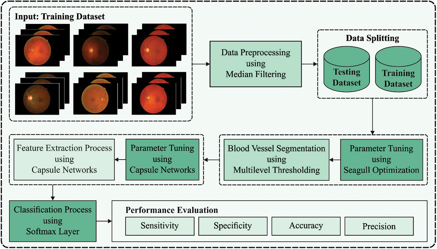
Figure 1: Block diagram of BVS-DLC model

3.1 Image Pre-processing Using MF Technique

At the beginning stage, the MF technique is applied to pre-process the input DR image to eradicate the existence of noise. The MF is the first kind of non-linear filter. It is highly efficient in eliminating impulse noise, the “salt, and pepper” noise, in the images. The concept of median filter is to replace the grey level of all the pixels with the median of the grey level in a neighbourhood of the pixel, rather than employing the typical process. For median filtering, they list the pixel value, determine kernel size, covered it with the kernel, and define the median levels. When the kernels cover even numbers of pixels, the average of 2 median values is employed. Beforehand imitating median filtering, 0’s should be padded all over the column and row edges. Therefore, edge distortion is presented at image boundary. The median filter using 3 * 3 kernels is employed for filtering the impulse noise. The enhanced image has a major quality enhancement. But the enhanced image seems smoothed, hence, the higher frequency data is minimized. Consider that a large size kernel isn’t suitable for median filtering, since for a large set of pixels the median values deviate from the pixel values.

3.2 Blood Vessel Segmentation

Once the preprocessing is done, the next stage is to segment the blood vessels using optimal Kapur’s entropy technique. The concepts of entropy criterion has been presented by Kapur et al. in 1980. So far, it is extensively used in defining an optimum threshold value in histogram based image segmentation. Like Otsu model, the original entropy criterion has been proposed for bi-level threshold. Also, it is expanded for solving multi-level threshold problems. Consider bi-level threshold as an instance, the Kapur criterion functions are shown in the following equation:

H0=−∑i=0t(PRiω0)ln(PRiω0),H1=−∑i=t+1L−1(PRiω1)ln(PRiω1)(1)

fKapur(t)=H0+H1(2)

whereas H0 & H1 represents the entropy value of C1 & C2, as well fKapur(t) denotes the objective function [20]. Assume a problem of defining n−1 threshold, the multi-level threshold is equated in the following:

fKopur(t1∗,t2∗,…,tn−1∗)=max{∑i=1n−1Hi}(3)

The Otsu and Kapur method has shown to be highly efficient for bi-level threshold in image thresholding also is expanded to multilevel thresholding for color and gray images. But, the optimal threshold is obtained through exhaustive searching models. This results in a sharp increase of the estimation time using the numbers of threshold. Therefore, assume Eq. (3) as the FF for gaining an optimum threshold {t1∗,t2∗,…,tn−1∗} and present an enhanced fruit fly optimization method, apply to solve multi-level thresholds. They designed a novel hybrid adoptive co-operative learning approach, and present a new solution system based on the concept that all dimensions of the solution vectors would be enhanced at the time one searches for maintaining the diversity of population. This method could efficiently shorten computational time, i.e., mainly appropriate for multi-level image thresholds. For determining the optimum threshold values, the SGO technique is applied.

Dhiman et al. [21] established a novel kind of bioinspired optimized technique, the seagull optimized technique with analyzing the biological features of seagulls. The seagulls live in groups, utilizing their intelligence for finding as well as attacking their prey. One of the vital features of seagulls has migration and aggressive performance. The mathematical process of the natural performance of seagulls is as follows.

In the migration technique, seagulls move from one place to another and meet 3 criteria’s:

Avoid collision: For avoiding collision with another seagull, variable A has been utilized for calculating the novel place of the search seagull.

Cs(t)=A×Ps(t),(4)

where Cs(t) implies the novel place that doesn’t conflict with another search seagull, Ps(t) signifies the present place of the search seagulls, t demonstrates the present iteration and A defines the motion performance of the search seagulls from the provided search space.

A=fc−(t×(fc/Maxiteration)),(5)

where t=0,1,2,…,Maxiteration,fc is manage the frequency of the variables, and their value drops in [2–0].

Best position: Then avoiding overlapping with another seagull, seagull is move in the way of the optimum place.

Ms(t)=B×(Pbs(t)−Ps(t)), where Ms(t) stands for the places of the search seagull. B defines the arbitrary number responsible to balance the global as well as local search seagulls [22].

B=2×A2×rd,(6)

where rd indicates the arbitrary number that lies from the range of 0 and 1.

Close to the best search seagull: Afterward, the seagull transfers to a place where it doesn’t collide with another seagull, it transfers in the way of an optimum place for reaching their novel place.

Ds(t)=|Cs(t)+Ms(t)|,(7)

where Ds(t) implies the optimum fit search seagulls.

The seagulls are always alteration their attack angle as well as speed in their migration. It can be utilized its wings and weight for maintaining heights. If the attacking prey, it can be move in spiral shape from the air. The motion performance in the, y, and z planes are explained as:

x=r×cos⁡(θ),(8)

y=r×sin⁡(θ),(9)

z=r×θ,(10)

r=u×eθv,(11)

where r refers the radius of spiral and θ implies the arbitrary angle from the range of [0,2π]. u and v demonstrate the correlation constants of spiral shape, and e refers the base of natural logarithm. The attack place of seagulls is constantly upgraded.

Ps(t)=Ds(t)×x×y×z+Pbs(t),(12)

where Ps(t) stores the optimum solutions and upgrades the place of another search seagull.

3.3 Feature Extraction Using Optimal CapsNet Technique

During feature extraction process, the SGO with CapsNet model is utilized as a feature extraction module. CapsNets demonstrate an entirely new kind of DL structure which tries to overcome restricts and disadvantages of CNN like insufficient explicit notion of entity and losing valuable data in max-pooling. An archetypal CapsNet is shallower with 3 layers, for instance, the Convld, PrimaryCaps, and DigitCaps layers. During this scenario, CapsNet has been robust for affine changing and requiring some trained information. Also, the CapsNet has resulted in different breakthroughs connected to spatial hierarchies amongst features. The capsule signifies a set of neurons. The activity of neurons surrounded in active capsule signifies the different properties of specific entity. Besides, the entire length of capsule demonstrates the presence of an entity and the orientation of capsule specify their property. Fig. 2 depicts the structure of CapsNet model. The CapsNet is a discriminatively trained multi-layer capsule model [23]. As the length of the resultant vector demonstrates the probabilities of existence, an outcome capsule was calculated utilizing a non-linear squashing function:

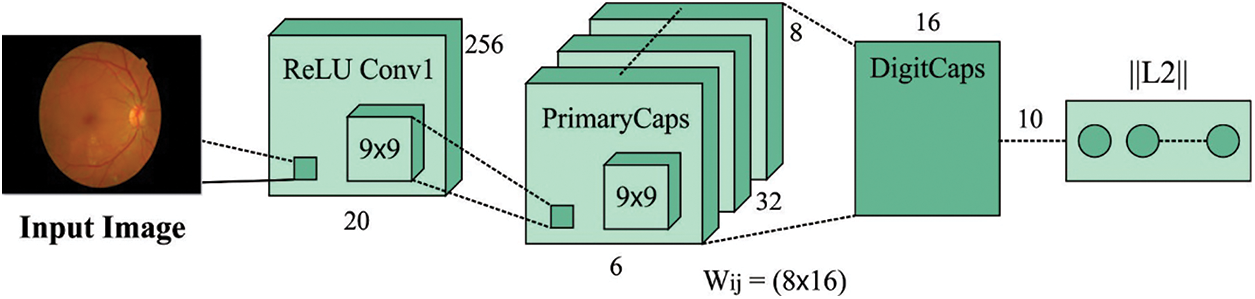
Figure 2: Structure of CapsNet model

vj=‖sj‖2ε+||sj‖2(13)

where vj refers the vector outcome of capsules j and sj is their entire input. The non-linear squashing function has been activation function for ensuring that the short vectors obtain shrunk to nearly 0 lengths and the long vector obtain shrunk to particular length in terms of ε.

sj=∑icijWijui(14)

An entire input to capsule sj is attained by multiplying the output ui of capsule with a weight matrix Wij that demonstrates a weighted sum entire forecasted vector in the capsules from the layer under. At this point, cij implies the coupling coefficients that is defined as iterative dynamic routing procedure:

cij=exp⁡(bij)∑kexp⁡(bik),(15)

where bij and bik refers the log prior probability amongst 2 coupled capsules. The entire length of the outcome vector signifies the forecasted probabilities. The distinct margin loss Lk to all capsules k are provided as:

Lk=Tkmax(0,m+−‖vk‖)2+λ(1−Tk)max(0,‖vk‖−m−)2,(16)

where Tk=1, m+=0.9, and m−=0.1 are 3 free parameters by default. λ allows the down-weighting of loss and uses make sure last convergences.

The hyperparameter optimization process of the CapsNet model can be performed by the use of SOA algorithm. The sharks are powerful olfactory receptors and have been defined its prey dependent upon this receptor. This technique performs dependent upon the subsequent conditions:

•   An injured fish is regarded that prey to sharks, as fish bodies distribute blood throughout the sea. Also, the injured fish is negligible speed related to sharks.

•   The blood has been distributed to the sea regularly, and the outcome of water flow could not be regarded to blood distribution.

•   All the injured fishes are assumed that one blood production resource to sharks; so, the olfactory receptors support sharks to define their prey.

•   The primary population of sharks is demonstrated as [X11,X21,…,XNP1], NP=population(size). All the solutions candidate or shark place are the subsequent modules dependent upon the subsequent formula:

Xi1=[xi,11,xi,21,…,xi,ND1],(17)

where Xi1 refers the primary place vector; xij1 stands for the jth dimensional of shark place, and ND implies the amount of decision variables. The primary velocity to sharks are demonstrated as Vi1=[vi,11,vi,21,…,vi,ND1]. The velocity modules have been assumed that dependent upon the subsequent formula:

Vi1=[vi,11,vi,21,…,vi,ND1],i=1,…NP(18)

where Vi1 signifies the primary velocity vector and vij1 denotes the jth dimensional of shark velocity. If the shark obtains superior odour intensity it changes faster near its prey. Therefore, when the odour intensity has been assumed that objective functions, the velocity modifies with the difference from the objective function dependent upon the subsequent formula as:

Vik=ηk.R1.∇(OF)|xik, where ηk denotes the number amongst [0, 1]; R1 represents the arbitrary numbers, and OF defines the objective function.

There is inertia in the shark progress that can be assumed in the shark velocity; therefore, Eq. (20) has been altered dependent upon the subsequent formula as [24]:

vi,jk=ηk.R1.∂(OF)∂xj+α.R2.vi,jk−1,(19)

where α refers the inertia coefficient and R2 defines the arbitrary value amongst [0, 1].

The sharks are a particular domain to velocity. Its maximal velocity is 80 km/hr, and its minimal velocity is 20 km/hr. Therefore, the velocity restrict has been assumed, and Eq. (21) has been changed dependent upon the succeeding formula:

|vi,jk|=min[|ηk.R1.∂(OF)∂xj|xi,jk+αk.R2.vi,jk−1|,|βk.vi,jk−1|],(20)

where βk stands for the velocity limiter. Afterward, the shark place has been upgraded dependent upon the subsequent formula:

Yik+1=Xik+VikΔtk′(21)

where Δtk represents the time step and Yik+1 denotes the novel place to the shark. The sharks are rotational movement operators. These operators’ represent that shark is escaping in the local optimum, and the shark place dependent upon rotational effort has been changed dependent upon the subsequent formula:

Zik+1,m=Yik+1+R3.Yik+1,m=1,…,M,(22)

where Zik+1,m refers the novel shark place and M signifies the amount of local search to the shark.

3.4 Image Classification

Finally, the softmax classifier is applied to assign appropriate class labels to the test DR images. In this model, they employ Softmax classifiers in classification, and its input is the feature i.e., learned from the feature learning model. In the classifier, the hypothetical text datasets have n text from k classes, in which the training set is formulated by {(x(1),y(1)),(x(2),y(2)),…,(x(n−1),y(n−1)),(x(n),y(n))} and x(i) represent the ith training texts, and y represent dissimilar classes (y(i)∈{1,2,…,k−1,k}). The key objective of this method is to evaluate the likelihood of x belong to the tag class, for the provided training set x. Now, function is expressed in the following equation

hθ(x(i))=[P(y(i)=1|x(i);θ)P(y(i)=2|x(i);θ)⋮P(y(i)=k|x(i);θ)]

=1∑j=1keθjTx(i)[eθ1Tx(i)eθ2Tx(i)⋮eθkTx(i)].

Every sub vector of vector hθ(x(i)) represent the likelihood values whose x belong to dissimilar tag classes, and the likelihood values should be standardized, thus the amount of likelihood values of each subsector is 1. And θ1,θ2,…,θk−1,θk∈Rn+1 represent the parameter vector, correspondingly [25]. Afterward receiving θ, attain the formerly considered function hθ(x). It is employed for calculating the likelihood values that text x belongs to every class. The class that has the largest likelihood values is the last result with the classifier method.

4  Experimental Validation

The performance of the BVS-DLC technique can be examined using MESSIDOR dataset [26], which contains different stages of DR and healthy images. Few of the sample retinal fundus images are depicted in Fig. 3.

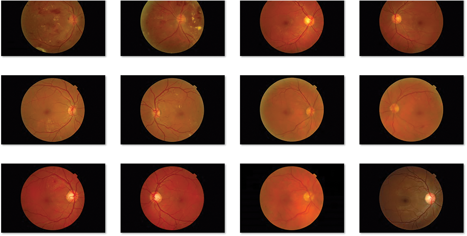
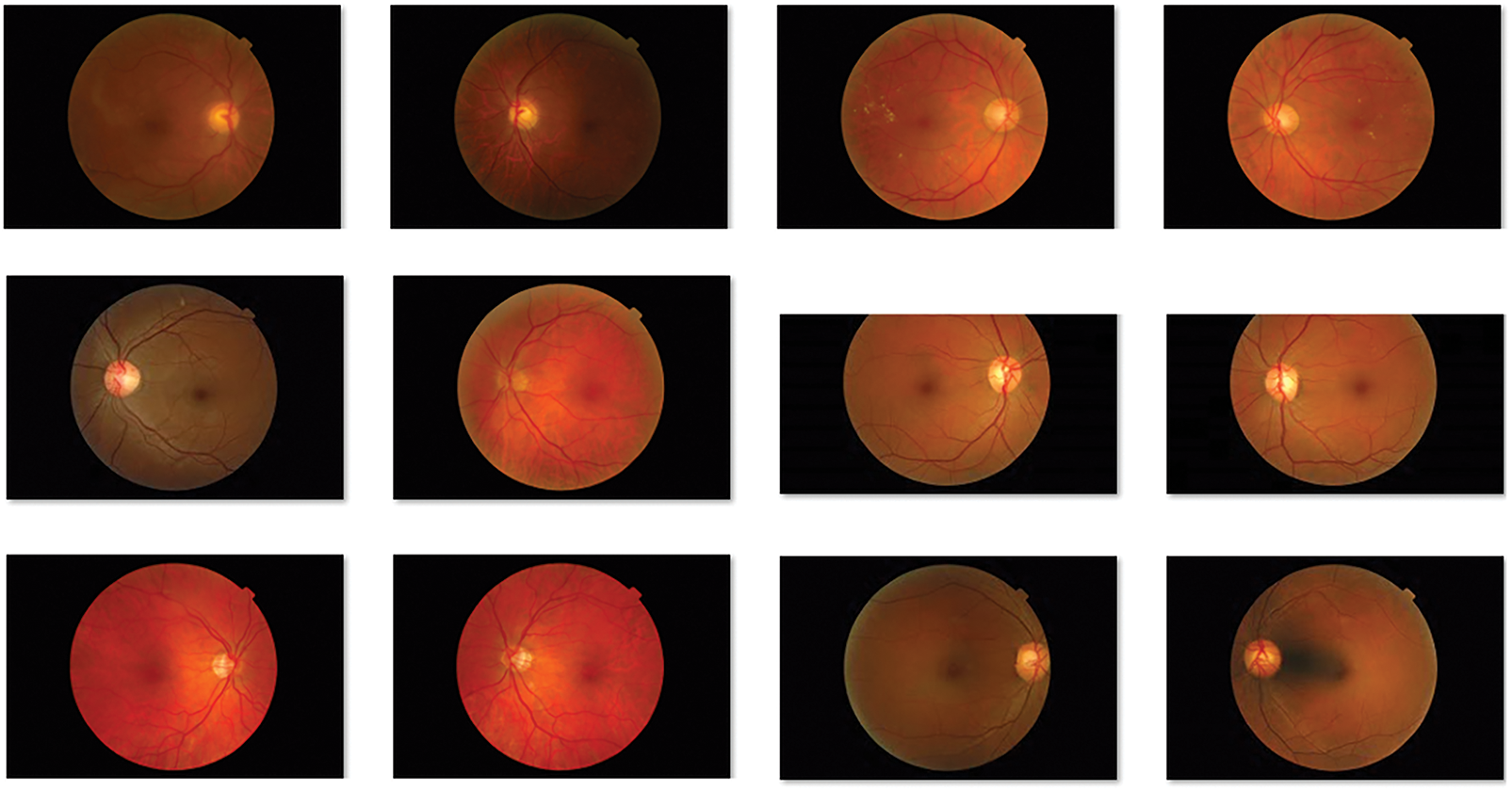
Figure 3: Sample retinal fundus images

An illustration of the segmented retinal fundus images is shown in Fig. 4 and the blood vessels can be clearly seen in the image. Therefore, the presented segmentation technique has accomplished proficient results on the applied images.

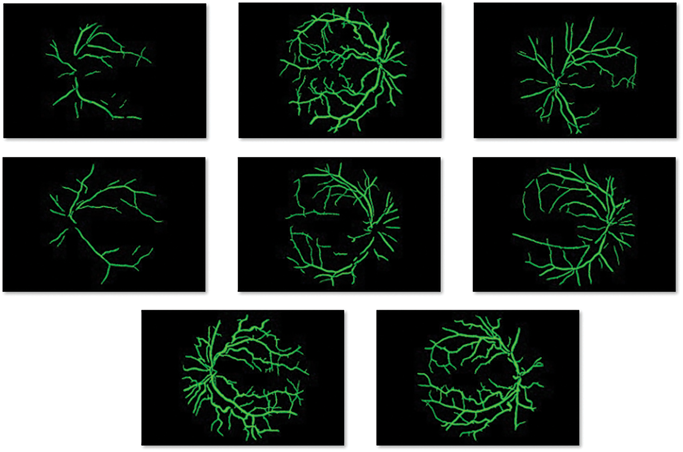
Figure 4: Blood vessel segmented image

The confusion matrix offered by the BVS-DLC technique under training/testing of 80:20 is depicted in Fig. 5. The results demonstrated that the BVS-DLC technique has properly categorized 544 images into Normal, 152 images into Stage 1, 246 images into Stage 2, and 253 images into Stage 3.

Figure 5: Confusion matrix of BVS-DLC model on training/testing dataset (80:20)

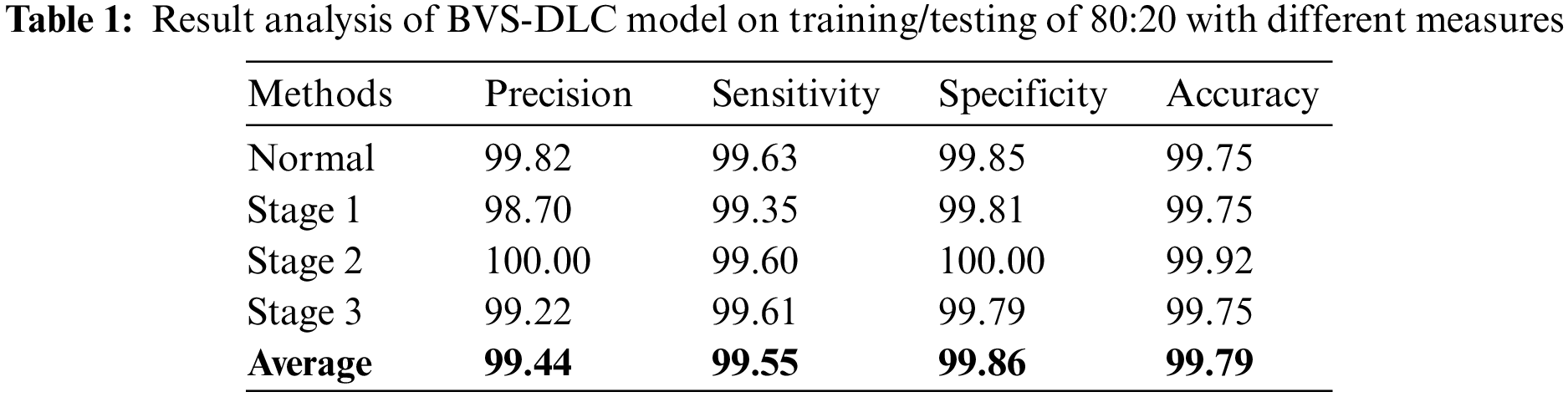
Table 1 portray the DR classification results of the BVS-DLC technique on the training/testing of 80:20. The results have shown that the BVS-DLC technique has gained effective results on the classification of distinct DR and healthy classes. In addition, the BVS-DLC technique has resulted in a maximum average precision of 99.44%, sensitivity of 99.55%, specificity of 99.86%, and accuracy of 99.79%.

The training and validation accuracy analysis of the BVS-DLC method is given in Fig. 6. The outcomes reported that the accuracy value tends to increase with a maximum in epoch count. Besides, the validation accuracy is significantly superior to the training accuracy.

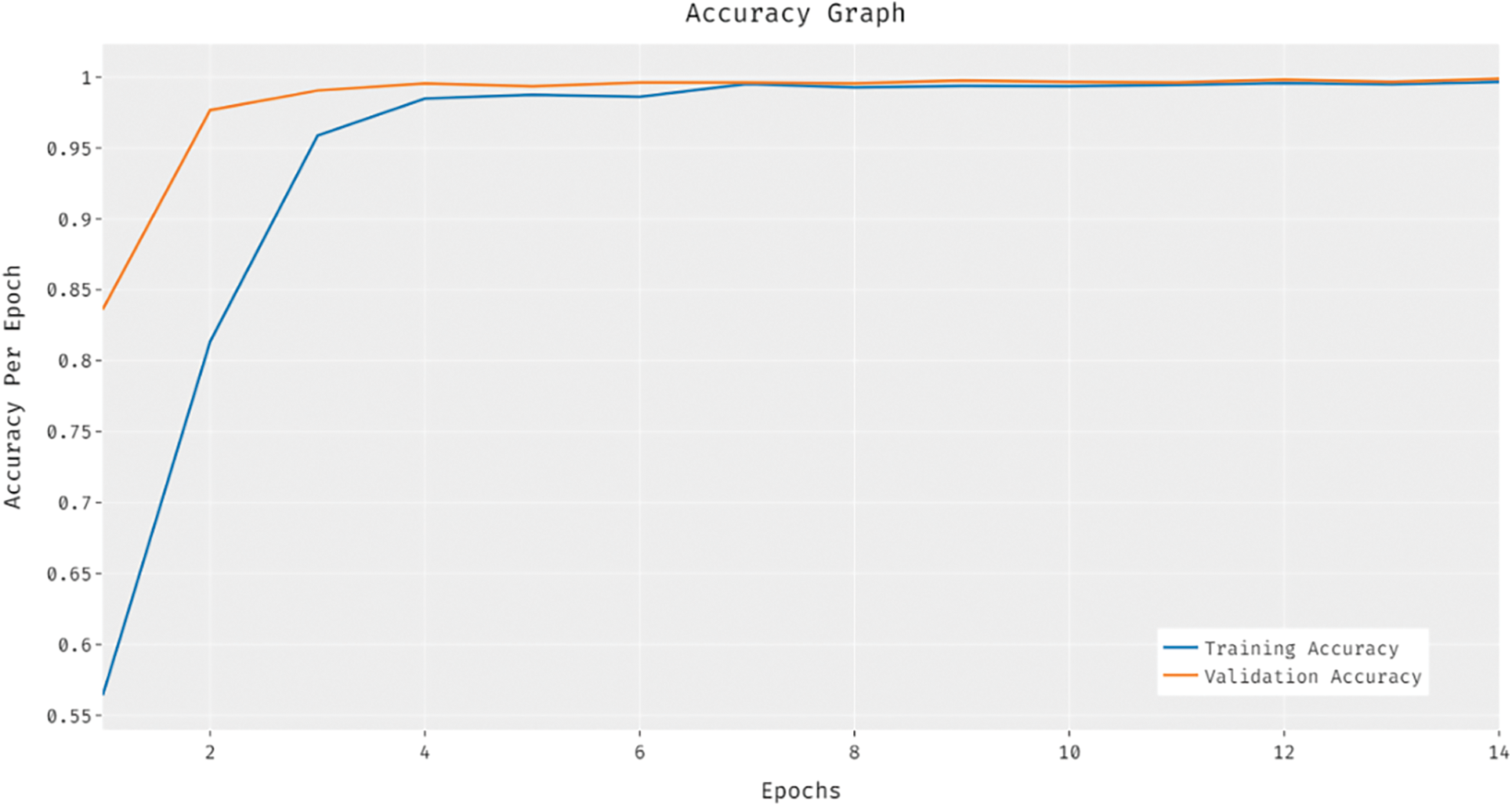
Figure 6: Accuracy analysis of BVS-DLC model

Fig. 7 showcases the training and validation loss analysis of the BVS-DLC method. The outcomes exhibited that the loss value is established for reducing with growth in number of epochs. In addition, the validation loss is noticeably minimum compared to the training loss.

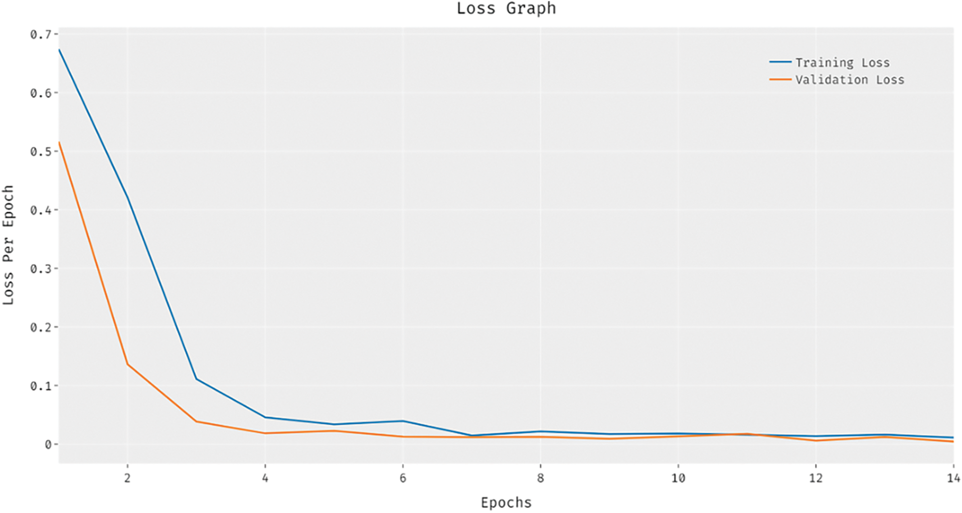
Figure 7: Loss analysis of BVS-DLC model

The confusion matrix obtainable by the BVS-DLC approach under training/testing of 70:30 is showed in Fig. 8. The outcomes outperformed that the BVS-DLC manner has properly categorized 542 images into Normal, 151 images into Stage 1, 245 images into Stage 2, and 252 images into Stage 3.

Figure 8: Confusion matrix of BVS-DLC model on training/testing dataset (70:30)

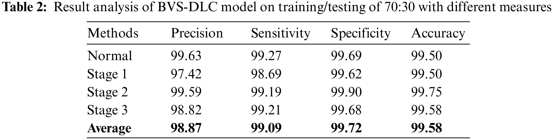
Table 2 depict the DR classification results of the BVS-DLC algorithm on the training/testing of 70:30. The outcomes depicted that the BVS-DLC manner has reached effectual outcomes on the classification of distinct DR and healthy classes. Besides, the BVS-DLC methodology has resulted in a maximal average precision of 98.87%, sensitivity of 99.09%, specificity of 99.72%, and accuracy of 99.58%.

The confusion matrix existing by the BVS-DLC technique in training/testing of 60:40 is demonstrated in Fig. 9. The results portrayed that the BVS-DLC method has properly categorized 541 images into Normal, 151 images into Stage 1, 244 images into Stage 2, and 252 images into Stage 3.

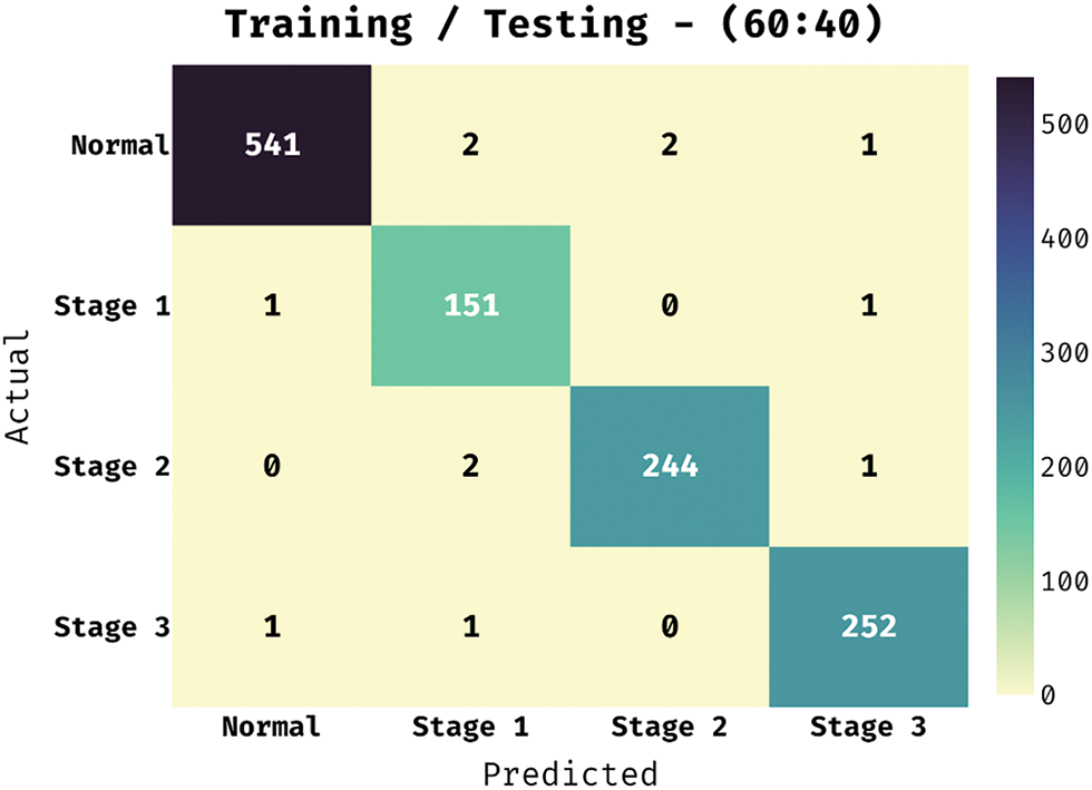
Figure 9: Confusion matrix of BVS-DLC model on training/testing dataset (60:40)

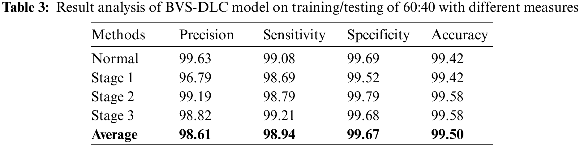
Table 3 illustrate the DR classification outcomes of the BVS-DLC manner on the training/testing of 60:40. The outcomes exhibited that the BVS-DLC algorithm has reached effectual outcomes on the classification of different DR and healthy classes. Moreover, the BVS-DLC algorithm has resulted in a higher average precision of 98.61%, sensitivity of 98.94%, specificity of 99.67%, and accuracy of 99.50%.

Finally, a comprehensive comparative results analysis [26–27] of the BVS-DLC technique is provided below. A sensitivity analysis of the BVS-DLC with existing techniques is provided in Fig. 10. The figure reported that the ADR-PCA and SIFT-FV-PCA techniques have offered lower sensitivity of 96% and 97% respectively. Meanwhile, the GLCM-SVM, HEDFD, and SVM-NN techniques have demonstrated moderately closer sensitivity of 98%, 98%, and 98% respectively. Although the FCM-SNN and DWT-PCA techniques have resulted in a competitive sensitivity of 99% and 99%, the presented BVS-DLC technique has accomplished a higher sensitivity of 99.55%.

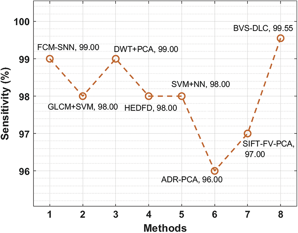
Figure 10: Sensitivity analysis of BVS-DLC model with recent approaches

Next, a specificity analysis of the BVS-DLC with existing manners is given in Fig. 11. The figure described that the SVM+NN and HEDFD methods have presented lesser specificity of 83% and 88% correspondingly. In the meantime, the DWT+PCA, GLCM+SVM, and SIFT-FV-PCA methods have showcased moderately closer specificity of 88%, 89%, and 89% correspondingly. While the FCM-SNN and ADR-PCA methods have resulted in a competitive specificity of 91% and 93%, the projected BVS-DLC method has accomplished a superior specificity of 99.86%.

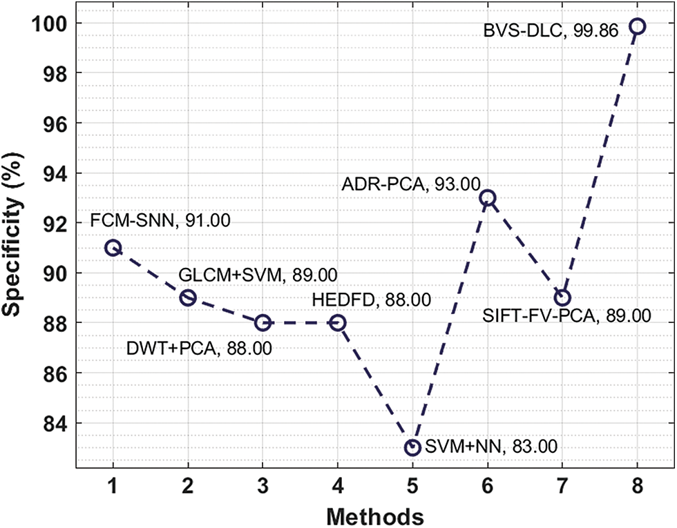
Figure 11: Specificity analysis of BVS-DLC model with recent approaches

Finally, an accuracy analysis of the BVS-DLC with recent algorithms is given in Fig. 12. The figure stated that the GLCM+SVM and SVM+NN systems have accessible least accuracy of 82% and 89.60% respectively. Followed by, the SIFT-FV-PCA, FCM-SNN, and HEDFD methods have showcased moderately closer accuracy of 91.03%, 93%, and 94.60% correspondingly. Afterward, the DWT+PCA and ADR-PCA manners have resulted in a competitive accuracy of 95% and 95.26%, the projected BVS-DLC methodology has accomplished an increased accuracy of 99.79%.

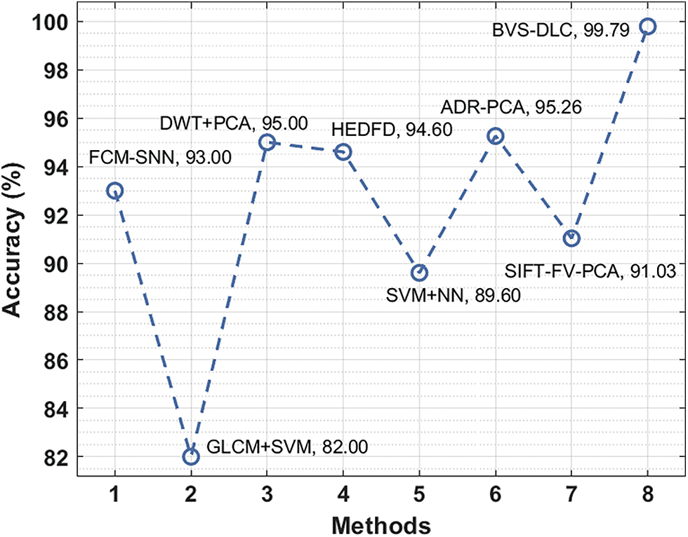
Figure 12: Accuracy analysis of BVS-DLC model with recent approaches

After examining the above results and discussion, it can be concluded that the BVS-DLC technique has been utilized as a proficient tool for DR diagnosis.

5  Conclusion

In this study, an intelligent BVS-DLC model is developed to diagnose DR at the earlier stage. The BVS-DLC model involves different stages of operations namely MF based pre-processing, optimal Kapur’s entropy based segmentation, CapsNet based feature extraction, SOA based hyperparameter optimization, and softmax based classification. The use of SGO algorithm for threshold value selection and SOA for hyperparameter tuning process helps to boost the overall DR diagnosis outcome. An extensive experimental analysis takes place using the MESSIDOR dataset and the projected BVS-DLC methodology has accomplished an increased accuracy of 99.79%. The simulation results ensured the better performance of the proposed model compared to other existing techniques interms of several measures. In future, advanced DL based segmentation techniques with ML based classifiers can be applied to improve the overall performance of the BVS-DLC technique.

Acknowledgement: The authors extend their appreciation to the deputyship for Research & Innovation, Ministry of Education in Saudi Arabia for funding this research work through the project number (IFP-2020-66).

Funding Statement: The authors received no specific funding for this study.

Conflicts of Interest: The authors declare that they have no conflicts of interest to report regarding the present study.

References

1. N. Tsiknakis, D. Theodoropoulos, G. Manikis, E. Ktistakis, Q. Boutsora et al., “Deep learning for diabetic retinopathy detection and classification based on fundus images: A review,” Computers in Biology and Medicine, vol. 2, no. 6, pp. 104599–104612, 2022. [Google Scholar]
2. J. Alicia, K. Jenkins, V. Mugdha, M. Anandwardhan, A. Hardikar et al., “Biomarkers in diabetic retinopathy,” Rev. Diabet, Stud.: Registered Deviation Studies, vol. 12, no. 1, pp. 159–169, 2015. [Google Scholar]
3. S. Hamid, S. Safi, A. Hafezi-Moghadam and A. Hamid, “Early detection of diabetic retinopathy,” Survey Of Ophthalmology, vol. 63, no. 5, pp. 601–608, 2018. [Google Scholar]
4. C. Changyow, A. Kwan, A. Amani and K. Fawzi, “Imaging and biomarkers in diabetic macular edema and diabetic retinopathy,” Current Diabetes Reports, vol. 19, no. 10, pp. 1–10, 2019. [Google Scholar]
5. P. I. Burgess, I. J. C. MacCormick, S. P. Harding, A. Bastawrous, N. Beare et al., “Epidemiology of diabetic retinopathy and maculopathy in africa: A systematic review,” Diabetes Medical, vol. 30, no. 4, pp. 399–412, 2013. [Google Scholar]
6. M. R. K. Mookiah, U. R. Acharya, C. K. Chua, C. M. Lim and A. Laude, “Computer-aided diagnosis of diabetic retinopathy: A review,” Computiational Biololgy Medical, vol. 43, no. 12, pp. 2136–2155, 2013. [Google Scholar]
7. L. Dai, L. Wu, H. Cai, C. Wu, Q. Kong et al., “A deep learning system for detecting diabetic retinopathy across the disease spectrum,” Nature Communications, vol. 12, no. 1, pp. 1–11, 2013. [Google Scholar]
8. I. Qureshi, J. Ma and Q. Abbas, “Recent development on detection methods for the diagnosis of diabetic retinopathy,” Symmetry, vol. 11, no. 6, pp. 749–756, 2019. [Google Scholar]
9. V. Gulshan, L. Peng, M. Coram, M. C. Stumpe, D. Wu et al., “Development and validation of a deep learning algorithm for detection of diabetic retinopathy in retinal fundus photographs,” Jama, vol. 316, no. 22, pp. 2402–2410, 2016. [Google Scholar]
10. K. Parthiban and K. Venkatachalapathy, “Internet of Things and cloud enabled hybrid feature extraction with adaptive neuro fuzzy inference system for diabetic retinopathy diagnosis,” Journal of Computational and Theoretical Nanoscience, vol. 17, no. 12, pp. 5261–5269, 2020. [Google Scholar]
11. B. B. Narhari, B. K. Murlidhar, A. D. Sayyad and G. S. Sable, “Automated diagnosis of diabetic retinopathy enabled by optimized thresholding-based blood vessel segmentation and hybrid classifier,” Bio-Algorithms and Med-Systems, vol. 17, no. 1, pp. 9–23, 2021. [Google Scholar]
12. Y. Wu, Y. Xia and V. Cai, “NFN+: A novel network followed network for retinal vessel segmentation,” Neural Networks, vol. 126, no. 5, pp. 153–162, 2020. [Google Scholar]
13. J. Jayanthi, T. Jayasankar, N. Krishnaraj, N. Prakash and K. Vinoth Kumar, “An intelligent particle swarm optimization with convolutional neural network for diabetic retinopathy classification model,” Journal of Medical Imaging and Health Informatics, vol. 11, no. 3, pp. 803–809, 2021. [Google Scholar]
14. V. Sathananthavathi and G. Indumathi, “Encoder enhanced atrous (EEA) unet architecture for retinal blood vessel segmentation,” Cognitive Systems Research, vol. 67, no. 4, pp. 84–95, 2021. [Google Scholar]
15. G. Arias, M. E. M.Santos, D. P. Borrero and M. J. V.Vazquez, “A new deep learning method for blood vessel segmentation in retinal images based on convolutional kernels and modified U-Net model,” Computer Methods and Programs in Biomedicine, vol. 205, no. 5, pp. 106081–106093, 2021. [Google Scholar]
16. H. Boudegga, Y. Elloumi, M. Akil, M. H. Bedoui and A. B. Abdallah, “Fast and efficient retinal blood vessel segmentation method based on deep learning network,” Computerized Medical Imaging and Graphics, vol. 90, no. July (4), pp. 101902–101924, 2021. [Google Scholar]
17. J. Vaishnavi, S. Ravi and A. Anbarasi, “An efficient adaptive histogram based segmentation and extraction model for the classification of severities on diabetic retinopathy,” Multimedia Tools and Applications, vol. 79, no. 41, pp. 30439–30452, 2020. [Google Scholar]
18. I. Atli and O. S. Gedik, “Sine-Net: A fully convolutional deep learning architecture for retinal blood vessel segmentation,” Engineering Science and Technology, an International Journal, vol. 24, no. 2, pp. 271–283, 2021. [Google Scholar]
19. L. Hakim, M. Kavitha, M. Yudistira and T. Kurita, “Regularizer based on euler characteristic for retinal blood vessel segmentation,” Pattern Recognition Letters, vol. 2, no. 10, pp. 321–335, 2019. [Google Scholar]
20. G. Ding, F. Dong and M. Zou, “Fruit fly optimization algorithm based on a hybrid adaptive-cooperative learning and its application in multilevel image thresholding,” Applied Soft Computing, vol. 84, no. 4, pp. 105704–105716, 2019. [Google Scholar]
21. G. Dhiman, K. Kumar and V. Seagull, “Optimization algorithm: Theory and its applications for large-scale industrial engineering problems,” Knowledge Based System, vol. 165, no. 25, pp. 169–196, 2019. [Google Scholar]
22. K. Chen, X. Li, Y. Zhang, Y. X. Xiong and F. Zhang, “A novel hybrid model based on an improved seagull optimization algorithm for short-term wind speed forecasting,” Processes, vol. 9, no. 2, pp. 387–398, 2021. [Google Scholar]
23. F. Deng, F. Pu, S. Chen, X. Shi, Y. Yuan et al., “Hyperspectral image classification with capsule network using limited training samples,” Sensors, vol. 18, no. 9, pp. 3153–3168, 2018. [Google Scholar]
24. Z. M. Yaseen, M. Ehteram, M. Hossain, C. M. Binti Koting, S. Mohd et al., “A novel hybrid evolutionary data-intelligence algorithm for irrigation and power production management: Application to multi-purpose reservoir systems,” Sustainability, vol. 11, no. 7, pp. 1953–1964, 2019. [Google Scholar]
25. W. Aziguli, Y. Zhang, Y. Xie, Y. Zhang, D. Luo et al., “A robust text classifier based on denoising deep neural network in the analysis of big data,” Scientific Programming, vol. 4, no. 12, pp. 1–12, 2017. [Google Scholar]
26. S. Stephan, T. Jayasankar and K. Vinoth Kumar, “Motor imagery eeg recognition using deep generative adversarial network with EMD for BCI applications,” Technical Gazette, vol. 29, no. 1, pp. 92–100, 2022. [Google Scholar]
27. R. F. Mansour, “Deep-learning-based automatic computer-aided diagnosis system for diabetic retinopathy,” Biomedical Engineering Letters, vol. 8, no. 1, pp. 41–57, 2018. [Google Scholar]
Cite This Article
Copyright © 2023 The Author(s). Published by Tech Science Press.
This work is licensed under a Creative Commons Attribution 4.0 International License , which permits unrestricted use, distribution, and reproduction in any medium, provided the original work is properly cited.
Downloads
Citation Tools