Xception-Fractalnet: Hybrid Deep Learning Based Multi-Class Classification of Alzheimer’s Disease

1  Introduction

Alzheimer’s disease (AD) is an illness that affects the brain and causes it to deteriorate, which is a neurological state. In this, the cells in the brain die, causing cognitive impairment and memory loss. It is one of the most frequent types of dementia, that has a significant detrimental influence on the social and personal lives of people [1–3]. The memory-related neurological illness is commonly known as dementia and AD is the most frequent kind. As per the 2015 World Alzheimer’s information, around 50 million humans are affected by dementia, with AD accounting for 70%–80% of occurrences. According to estimates, 131.5 million individuals worldwide would be affected by AD in 2050 [4–7]. The global prevalence of AD is worrying because every three seconds one person is affected by this disease.

Chemicals, head injuries, and genetic environmental factors are some of most important causes of AD. Behavior and mood instability, communication and recognition problems, learning issues, and memory loss are common signs of AD [8–11]. It triggers brain cell death, resulting in thinking, memory, and cognitive impairment. It progresses over time and is labeled as a pre-clinical stage. The rate at which this disease progresses varies from patient to patient, but it has a terrible outcome. It produces a behavioral abnormality that affects the patient’s social functionality [11–13]. The normal onset and signs of this illness appear beyond the age of 65, however, it can develop earlier in life and the symptoms may not appear until this age.

The hippocampus and cerebral cortex sizes are reduced in AD patients’ brains. However, the ventricle’s size is increased in the brain. If the hippocampus size is reduced, the episodic and spatial memory parts are damaged. It also decreases the connectivity between the body and brain [14–16]. Cell death and damage of synapses and neuron endings occur as a result of hippocampus shrinkage. Communication problems in short-term memory, judgment, and planning have been found as a result of neuronal uncertainty.

AD is a multiclass classification issue, the majority of existing research is focused on binary classification, in which either an individual has AD or does not. However the more significant part of diagnosis should be identifying the stage of the disease [17–19]. Different clinical examinations are required for the diagnosis of AD, resulting in a vast amount of data samples. As a result, manual data analysis for detecting AD stages is not possible. Many Computer-Aided Diagnosis Systems (CADS) have been created by researchers to accurately detect and classify the retrieved aspects linked to AD, more time and effort from human experts are required to process the extracted features.

Various studies have employed a variety of machine learning algorithms to categorize Alzheimer’s disease using neuroimaging data. However the, conventional machine learning algorithms necessitate the human extraction of features before categorization. User-defined features-based approaches have some drawbacks one such is the failure to select the unique features related to the problem [20–24]. For automatic feature extraction and analysis of brain data, deep learning techniques have been recently utilized in the area of neuro-imaging with the use of graphical processing units and improved processing power. The deep learning models attained the best results due to their automatic feature extraction ability.

To counter the drawbacks of traditional methods in classification and feature extraction, in this paper, an effective hybrid Xception-Fractalnet-based deep learning technique is proposed for the Alzheimer’s disease classification system. It classifies AD into five classes namely Cognitively Normal (CN), Late Mild Cognitive Impairment (LMCI), Early Mild Cognitive Impairment (EMCI), Mild Cognitive Impairment (MCI), and Alzheimer’s Disease (AD). Moreover, a Unet++ based effective segmentation network is applied to improve the classification system’s performance and identify AD in the beginning. Compared to other deep learning techniques, the fractal architecture contains different levels of node interaction. Complex tasks are efficiently handled by this network due to its networks’ constant connection among various layers. Further, Unet++ contains dense and nested skip connections which provide an accurate semantic segmentation map. Therefore, this proposed hybrid approach achieves superior results than existing techniques in AD segmentation and classification.

1.1 Contribution

The important contributions of this paper are listed in the following three aspects,

•   The deep learning-based new framework is suggested to solve the direct five-class classification task in AD which is much more difficult than the traditional single or multiple binary classifications.

•   Depthwise separable convolution in the Xception architecture is developed to enhance the local features and retrieve discriminative features of critically modified microstructures in the brain.

•   The suggested model considerably improves the accuracy of the Alzheimer’s Disease MRI diagnosis by incorporating hyperparameter optimization through a metaheuristic approach.

•   An extensive analysis of the Alzheimer’s disease Neuroimaging Initiative (ADNI) data set revealed a significant performance improvement compared to benchmark techniques.

The remaining part of this paper is organized as follows: In Section 2, the related work about AD classification is discussed. The motivation for the work is presented in Section 3. In Section 4, the procedure and the key technology of the proposed approach are described. The evaluation metrics and experimental of the approach are shown in Section 5. Limitations and future scope are displayed in Section 6 and the conclusion is drawn in the last Section.

2  Literature Review

In recent years, many new frameworks have been developed that support tissue segmentation and AD categorization. Some of them are discussed in this section.

2.1 Threats to Validity

This part contains papers that (1) address any deep learning or machine learning approach and (2) analyze works on the categorization of AD and brain tissue segmentation, and (3) analyze performance assessment metrics. To find the peer-reviewed academic publications, we combined several words, like “multi-class classification of AD,” “classification of AD with deep learning,” and “AD tissue segmentation”, “Alzheimer’s disease classification”. We have concentrated on recent technological advancements made in 2021 and 2022. The six databases such as SpringerLink, ScienceDirect, IEEE Xplore, and Scopus have been our primary focus. The above-mentioned online databases have been selected as they provide some important complete conference papers and peer-reviewed articles in the area of AD classification with deep learning and machine learning techniques. Relevant papers were discovered by analyzing the title and abstract. For both forward and backward searching, Google Scholar was employed.

2.2 Tissue Segmentation

Li et al. [25] employed the MultiRes + UNet network to successfully segregate the brain tissue. With the use of MultiRes blocks and Res path structures, the authors reduced the amount of memory in the network. To remove the noise from the brain images, a non-local-based attention technique was included in this system. Finally, the binary classification among NC, LMCI, EMCI, and AD classes was conducted by the VoxCNN approach.

For brain tissue segmentation, the U-net technique was proposed by Basnet et al. [26]. To decrease the parameters of the network and increase the gradient glow, residual skip connections and densely linked convolution layers were used in this network. DSC loss, cross-entropy loss, and combined loss functions were utilized. The authors used the IBSR18 dataset for performance assessment with average surface distance, DSC, and modified Hausdorff distance metrics.

Another approach based on U-net was presented by Long et al. [27] for the segmentation of brain tissues. In this, the researchers used Channel Dimension and multi-scale-based u-net. In the encoding section, a multi-branch pooling-based information extractor was used to obtain the spatial features of the image and in the decoding section, a multi-branch dense prediction-based information extractor was utilized to gather all the spatial features as possible. the authors evaluated the performance of the approach based on Hausdorff Distance, DSC, and Absolute Volume Difference metrics.

Bhuvaneswari et al. [28] performed an AD segmentation and classification process. For this, they implemented skull stripping as the preprocessing operation on the dataset. Then segment-based segmentation was conducted to identify cerebrospinal fluid, hippocampus, cortex thickness, gyri and sulci contour, cortex surface, white matter, and grey matter features of the AD patient’s brain parts. Afterward, the Resnet-101-based classification network was implemented to perform the classification process. To analyze the effectiveness of the technique, accuracy, precision, specificity, and sensitivity metrics were used.

Xu et al. [29] modified the CNN architecture with the inception blocks to perform the classification task. These inception blocks were used to extract the deep features from the segmented grey matter slices. For grey matter segmentation, they implemented the enhanced independent component analysis technique. For the classification process, they choose particular informative slices from the whole volume of MRI images with the use of entropy. Then the pre-processing was conducted before the segmentation process. In this process, the unwanted tissues from the slices were removed using the skull stripping technique. Finally, the results were analyzed using the standard performance metrics and it is compared with existing state of art techniques.

Basheera et al. [30] developed a modified Tresnet-based deep learning technique to recognize three stages NC, MCI, and AD. Initially, in the pre-processing stage, the skull-removing process was performed by the FMRIB Software Library software with batch processing. Then the MRI images were segmented into white matter, grey matter, and Cerebro Spinal Fluid with the use of the SPM + cat12 tool kits in MATLAB. Finally, the segmented grey matter was taken by the modified Tresnet to classify the stages of AD.

2.3 Disease Classification

For AD classification, AbdulAzeem et al. [31] presented a CNN-based end-to-end framework. They classified both binary and multiclass classification. Five layers were included in this framework. The data acquisition was performed in the initial layer and the data augmentation and thresholding were performed in the second layer to improve the performance of training datasets. The cross-validation technique was implemented to train the CNN network in the third layer. Finally, the CNN was implemented in the fourth layer and the result was obtained in the final layer. For the optimization process, the Adam optimizer was implemented and the network weights were assigned by the Glorot Uniform weight initializer. For performance assessment, accuracy, precision, and recall metrics were used on the ADNI dataset and compared with existing state of art techniques.

Turkson et al. [32] proposed spiking deep CNN architecture for three binary classifications of AD such as NC vs. MCI, AD vs. MCI, and AD vs. NC. Initially, the MRI images were pre-trained by the unsupervised convolutional Spiking Neural Networks. Then the output of this network was processed by the supervised deep CNN for the classification process. The authors evaluate their techniques based on the standard performance metrics and compared the result with existing techniques such as Naïve Bayes, K-nearest neighbor (KNN), Support Vector Machine (SVM), Random Forest (RF), 3D CNN and sparse auto encoders.

Amini et al. [33] experimented with various machine learning techniques like RF, linear discrimination analysis (LDA), SVM, decision tree (DT), and KNN. To identify the severity of the AD was analyzed by the CNN framework. They utilized ADNI dataset for this research. For feature extraction, multitask techniques were implemented. Moreover, the Mini-Mental State Examination score was used to calculate the severity of the disease. This score includes severe, moderate, mild, and low categories.

To recognize and classify the stages of AD, Al-Adhaileh [34] implemented Restnet50 and AlexNet-19-based deep neural network methods. The author collected the MRI images from the Kaggle website for experimental evaluation. In this study, both binary (MCI-CN, AD-CN, and AD-MCI) and multi-class classification (AD-MCI and CN) were conducted. For performance assessment, Accuracy, Sensitivity, specificity, and AUC metrics were used and compared with existing techniques.

The Transfer learning-based deep CNN frameworks were discussed by Srinivas et al. [35] for the categorization of brain tumors. Three pre-trained networks such as Resnet-50, inception V3, and VGG-16 were analyzed for the diagnosis of brain tumor. Each testing stage included the addition of data preparation, data augmentation techniques, and predicted hyperparameter integral adjustment. Based on the accuracy, precision, recall, and F1-score criteria, performance assessments were made.

Yang et al. [36] performed the tumor prediction using CA125 based feature engineering technique. To increase the prediction capacity of the technique, various kinds of class imbalance techniques were utilized by the authors. They observed that the combination of SVM and Decision tree with SMOTE technique attained high prediction capacity in terms of specificity, sensitivity, AUC, and PPV.

Alam et al. [37] presented a decision support system based on fuzzy inference to identify several disorders. This system used symptoms of illness to identify new infections. It monitored the symptoms properly to identify the disease based on a fuzzy inference system. For each disease indicator, a distinct factor was utilized to forecast and calculate the severity of the projected disease.

Devnath et al. [38] reviewed several feature extraction and classification techniques presented in the previous 5 decades for disease detection. In this paper, it was observed that the majority of the experiments used conventional and standard machine learning techniques. Eight researchers used deep learning techniques as of this paper, and they performed better than other detection techniques. Therefore, it is found that deep learning techniques attained better performance in disease detection than traditional techniques.

3  Motivation of the Work

AD categorization using MRI image data is difficult as the MRI data contains higher variance in inconsistency, texture, contour, discontinuity among the tumor cells, and the normal area in the brain image. To diagnose the tumor effectively, automatic segmentation and classification are needed as manual tumor region detection takes a lot of time. Moreover, learning low dimensional representations while keeping the structural details of AD data and minimizing the impact of noise is difficult from the extracted features. Although many solutions have been put out in the past to address the segmentation and classification issues, a quick and effective solution is still required to enhance segmentation and classification performance. This has led us to suggest a deep learning-based hybrid strategy using MRI imaging modalities to get the best results in brain tissue segmentation and tumor classification.

4  Proposed Methodology

The working procedure of the proposed approach is detailed in this section. The algorithm of the proposed framework is based on five basic steps. The first stage is data pre-processing and augmentation, the second stage is input image segmentation, and the third and fourth stages are feature extraction and dementia classification. Initially, the input data are acquired from the ADNI dataset followed by the pre-processing methods implementation to eliminate noise and artifacts from data. Pre-processed image is then given into Unet++ based architecture for the segmentation of white matter, grey matter, hippocampus, and cerebrospinal fluid. Afterward, feature extraction and classification of AD are performed by Xception and fractal-net-based deep learning techniques. This technique classifies the AD into 5 classes. They are Cognitively Normal (CN), Late Mild Cognitive Impairment (LMCI), Early Mild Cognitive Impairment (EMCI), Mild Cognitive Impairment (MCI), and Alzheimer’s Disease (AD). The system architecture of this proposed work is shown in Fig. 1.

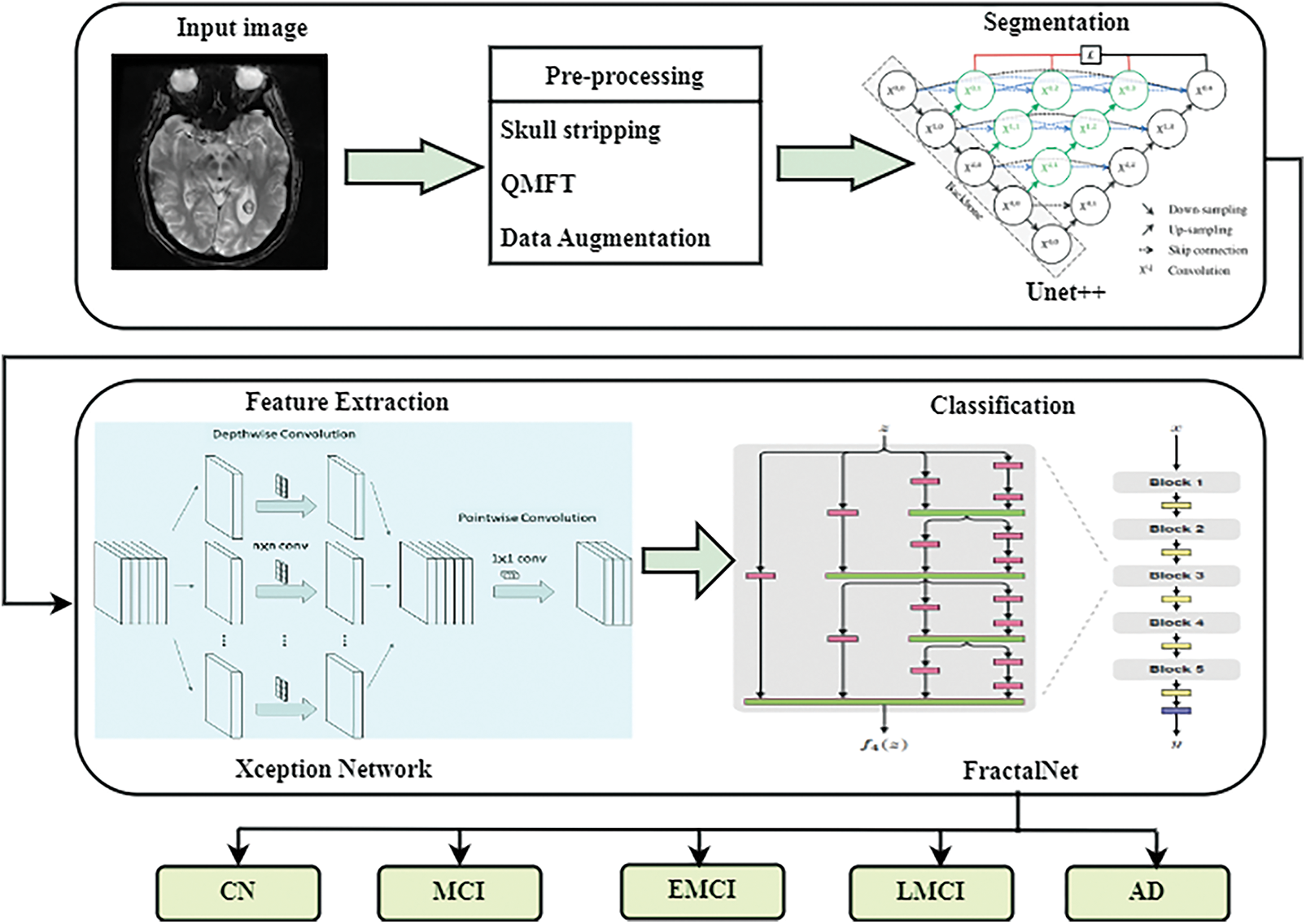
Figure 1: System architecture of the proposed system

4.1 Preprocessing

In image processing, pre-processing is the significant phase for smoothing, noise removal, and enhancement of images. In this paper, the skull stripping technique was implemented in the pre-processing stage to remove the skull in the brain as it was not part of the region of interest. Hence, skull stripping helped in obtaining better results. Afterward, the quantum matched-filter technique (QMFT) was applied to remove the low-level noise from the image. In this procedure, the essential and specific image features were separated by the active contour. Due to this, unwanted information like noise was removed, local thresholds could simultaneously identify extensive details by combining small and extensive features and read all columns and rows diagonally and linearly. Quantum reaches QMFT, which are used for the reduction of noise in MRI images. In addition, various data augmentations like shearing, flipping, rotation (45°), and brightness improvement were performed. Due to this, the amount of database images increased.

4.2 Segmentation

For AD classification, the segmentation of cerebrospinal fluid, hippocampus, white matter, and grey matter regions of the brain are the most significant parts. For this purpose, the Unet++ network was adapted and trained to segregate the above-mentioned brain regions from pre-processed images. To improve the process of segmentation, the dense block and convolutional layers were provided among the decoder and encoder. Compared to the Unit model, the unet++ architecture has some additions like deep supervision, dense skip connections, and redesigned skip pathways. This architecture contains convolution units, skip connections among convolution units, and up-sampling and down-sampling modules. Each node in this network receives the skip connections at the same level as all convolution units.

Initially, the pre-processed image was given as the input to the Unet++. The input image was then convolved by a convolution layer in the encoder path to obtain the feature map. This feature map passed through the skip routes and was sent to the decoder path’s corresponding convolution. Three convolution layers into a dense convolution block appeared in the skip pathway among the corresponding encoder and decoder nodes. Here, a concatenation layer is preceded by each convolution layer which combined the output from the up-sampled result of the lower dense block with the corresponding dense block’s previous convolution layer. The loss of semantic information among the two pathways is minimized with this structure. Down-sampling was done in the encoder path using a maximum pooling operation with a 2 kernel size and 1 stride. The feature map is half the size with this window and stride arrangement. The features were effectively extracted from the image using a down-sampling operation in the encoder path and the up-sampling was employed in the decoder pipeline to double the size of the feature map. Lastly, the segmentation mask was generated based on the final feature maps.

Let us assume that the output of node Yi,j is denoted by Yi,j, where i and j denote the downsampling and convolution layers respectively. The downsampling layers appear in the encoder path and the convolution layers appear in the skip pathway. The generation of feature maps by Yi,j is described as

xi,j={A(yi−1,j),j=0A[[y(i,k)]k=0j−1,u(yi+1,j−1)],j>0(1)

Here, the activation function associated with the 1-D convolution operation is represented by A(.), the up-sampling layer is denoted by u(⋅), and [⋅] represents the operation of concatenation. Nodes with level j = 0 received only one input from the encoder’s preceding layer, whereas nodes with level j > 0 received j + 1 inputs from both the up-sampling layer and skip connections. It’s important to note that the activation function is scaled exponential linear units (SeLUs) rather than ReLU, which allows for stronger regularisation approaches and more robust learning.

f(y)=λ{y,y>0α(exp⁡(y)−1),y≤0(2)

In this model, the deep supervision method was used to force the decoder blocks’ outputs to produce a valid segmentation map. Furthermore, the Unet++ training process’s loss function was based on the loss of categorical cross-entropy:

loss=−∑i=1kzilog(zi)(3)

Here, zi is the proportion of classes belonging to class i and k is the number of classes.

4.3 Feature Extraction

The segmented image was given as input to the exception framework for feature extraction. The Xception architecture is a modified version of the Inception architecture that uses Depth-wise separable convolutional modules instead of Inception modules. The feature extraction was formed by 36 convolutional layers which were separated into 14 modules in the Xception architecture. Each of the modules was surrounded by linear residual connections (excluding the last and first modules).

To extract features, the segmented pictures are first fed into the convolutional kernels of (3, 3, 64) and (3, 3, 128). The convolution layers’ calculations are as follows:

xjl=f(ujl)(4)

ujl=∑i∈Mjxil−1∗ki,jl+bjl(5)

Here, bl denotes the offset parameter, the output of the lth convolutional channel of the jth convolutional layer is denoted by xjl and the net activation of this channel is denoted by ujl, which is convolved and offset by the preceding xil−1 owned.

Second, the depthwise separable convolution is used to extract more features from the feature maps. To decrease the calculation complexity and the number of parameters, depthwise separable convolution is utilized. The connection layer then receives the produced two-dimensional feature map as input.

xl=f(ul)(6)

ul=wlxl−1+bl(7)

Here, the threshold offset term is denoted by bl, and the fully connected lth layer’s weight coefficient is denoted by wl. The gradient descent approach is then used to change the training error reduction’s direction.

δl=∂E∂ul(8)

Here, the variations among actual output and desired output’s square are represented by E, and the squared function error with a change in ul is denoted by δl. Finally, the feature map of the connected layer yielded a 2048-dimensional feature vector. For classification, the feature vector was fed into Fractalnet.

4.4 Classification

In this work, the classification of AD is conducted based on Fractalnet architecture. The feature vector obtained from the exception network is given as the input to the fractal net for classification. In this network, five fractal blocks and a pooling layer were consequently arranged.

FBC(N) represents the fractal block where C represents the number of columns in the block. In this work, Fractalnet with two columns is used. Therefore, in each fractal block, the number of convolution layers 2C–1 = 22–1 = 3. B * 2C–1 was the overall depth of the convolution layer. Here the number of fractal blocks was denoted by B. As fractal architecture used 5 fractal blocks, the entire amount of convolution layers in the framework was 3 * no of fractal blocks = 3 * 5 = 15. In addition, the results from this shallow network were substantially faster.

The base function of this architecture contains a convolution layer, batch normalization, and ReLU activation function. The following equation shows the convolution layer’s mathematical function.

Xsl=∑i,jWslXi,jl−1+Bsl(9)

Here, the outcome of the current layer ‘l’ for the ‘s’ filter is denoted by Xsl. Xi,jl−1 denotes the previous layer’s output, and the vertical and horizontal extent of a filter is denoted by j and i correspondingly. B and W denote the bias and kernel. After the convolution layer, batch normalization was applied to normalize the input, and the transformation of the input is provided in the following equation.

X^l−1=Xl−1−μσ2+ε(10)

Xl=αlX^l−1+βl(11)

Here, the shift parameters, learning rate, standard deviation, and mean are denoted β,α,σ,μ correspondingly.

A ReLU activation function is provided in the following equation

ReLU(Xl)=max(0,Xl)(12)

The coloration units are joined together to produce a fractal block with two columns using the join function. The Eq. (13) is used to calculate fractal blocks recursively.

FbC+1(N)=[(FbC∘FbC)(N)]⊕[conv(N)](13)

In the above equation, the number of columns are denoted by C, the join operation is denoted by ⊕ to calculate the mean of 2 convolution blocks, and the composition is denoted by ◦. Several inputs are combined into a single output unit by the Join layer. From input to output, there are 2C–1 convolution layers. To get a deeper network, this expansion rule is repeated. 2C–1 equals the fractal block’s depth. The fractal block with four columns has a depth of 24–1 = 15 convolution units.

The feature vector was fed into the fractal block, which had a joining layer and 3 convolution layers. The fractal block’s output was given to the pooling layer, which decreased the feature map’s dimension and the training parameters. The pooling layer and the fractal block sequence were repeated five times. Finally, the fully connected layer obtained the features followed by the softmax classifier which classified the classes of AD. To improve the performance of the classifier and reduce the error rate, the important parameters of Fractalnet such as learning rate, dropout rate, and batch size were optimized by the Emperor penguin optimization algorithm.

4.4.1 Emperor Penguin Optimization

In this section, the EPO technique is discussed to tune the hyperparameters of the Fractalnet model, which improves the classification performance of the proposed model. The purpose of parameter optimization is to alter the classifier’s hyperparameters to the point where the classification performance is maximized.

The EPO algorithm is based on the huddling behavior of emperor penguins (EPs) in Antarctica. Foraging is usually done in colonies by EPs. The huddling habit of the animals when foraging is an interesting characteristic. As a result, the primary goal is to decide on a talented mover from the ground in a mathematically sound manner. Following the temperature profile θ′, the distance between EPs(Xep) is determined. For reaching optimal values, the effective mover is represented, and the positions of other EPs are changed. The following are the steps involved in EPO. The EPs’ temperature profile is shown by

θ′=(θ−itermaxC−itermax)(14)

θ={01ifRn>0.5ifRn<0.5(15)

Here, C denotes the current round as determined by Iter max and Rn specifies the random number between 0 and 1: Because EPs tend to huddle together to maintain temperature, extra caution must be taken to safeguard them from nearby collisions. As a result, a set of two vectors (V→)(W→) whose values are computed as follows:

V→={P×(θ′+Xgrid(accuracy))×Rand0}−θ(16)

W→=Rand()(17)

Xgrid(accuracy)=|X→−X→ep|(18)

Here, the best result is denoted by X→, X→ep denotes other EP’s location, the movement parameter is represented by P, [0, 1] and || is Rand’s exact value.

D→=|{S(V→).X→(x)−W→.X→ep(x)}|(19)

S(V→)=(fe−C/v−e−c)2(20)

Eqs. (19) and (20) are used to calculate the distance between the EP and the optimal fittest searching agent. Eqs. (19) and (20) show the social forces that lead to EPs following the optimum searching agents, and e denotes the exponential function. The EPs’ position can be upgraded based on the optimum agents obtained using Eq. (21).

X→ep(X+1)=X→(x)−V→.D→ep(21)

The EP population is initialized in EPO using arbitrarily manufactured unique EPs.

5  Result and Discussion

In this section, the performance and efficiency of the proposed framework are assessed by several experiments on the ADNI dataset using typical performance metrics. Windows 10 operating system is used to train and test the proposed method with 16 GB of RAM and an Anaconda navigator. Keras is used to run all of the simulations, with Tensorflow as the backend.

5.1 Dataset Description

The data was gathered from the AD Neuroimaging Initiative (ADNI) database (adni.loni.usc.edu), which was utilized in several studies to classify Alzheimer’s disease. Dr. Michael W. Weiner founded ADNI in 2004 with the aid of public-private collaboration. The basic goals of ADNI were to investigate more reliable and sensitive methodologies on various diagnostic tools, such as structural MRI, PET, MRI, and clinical assessment, to track the early stages of AD and the course of MCI. 1296 MRI images were used in this study, divided into five categories: AD, LMCI, EMCI, MCI, and NC.

5.2 Training and Testing

The entire dataset was split into a training set (95%) and a testing set (5%). To train the segmentation and classification network, the SGD optimizer was employed. SGD can reach global minima and provide great training accuracy when using momentum. The number of columns in each fractal block in the fractal net were altered from 1 to 4. The training time of the network was increased when the number of columns increased. The model, on the other hand, provided an improved accuracy for fractal blocks with two columns while requiring significantly less training time. As a result, the proposed model employed fractal blocks with two columns, each of which was repeated five times.

The accuracy of the model was evaluated after it is applied to training data, and this was referred to as training accuracy. Testing accuracy is the accuracy when the testing data is applied to the model to obtain the result. As demonstrated in Fig. 2, the training and testing accuracy improved as the number of epochs increases.

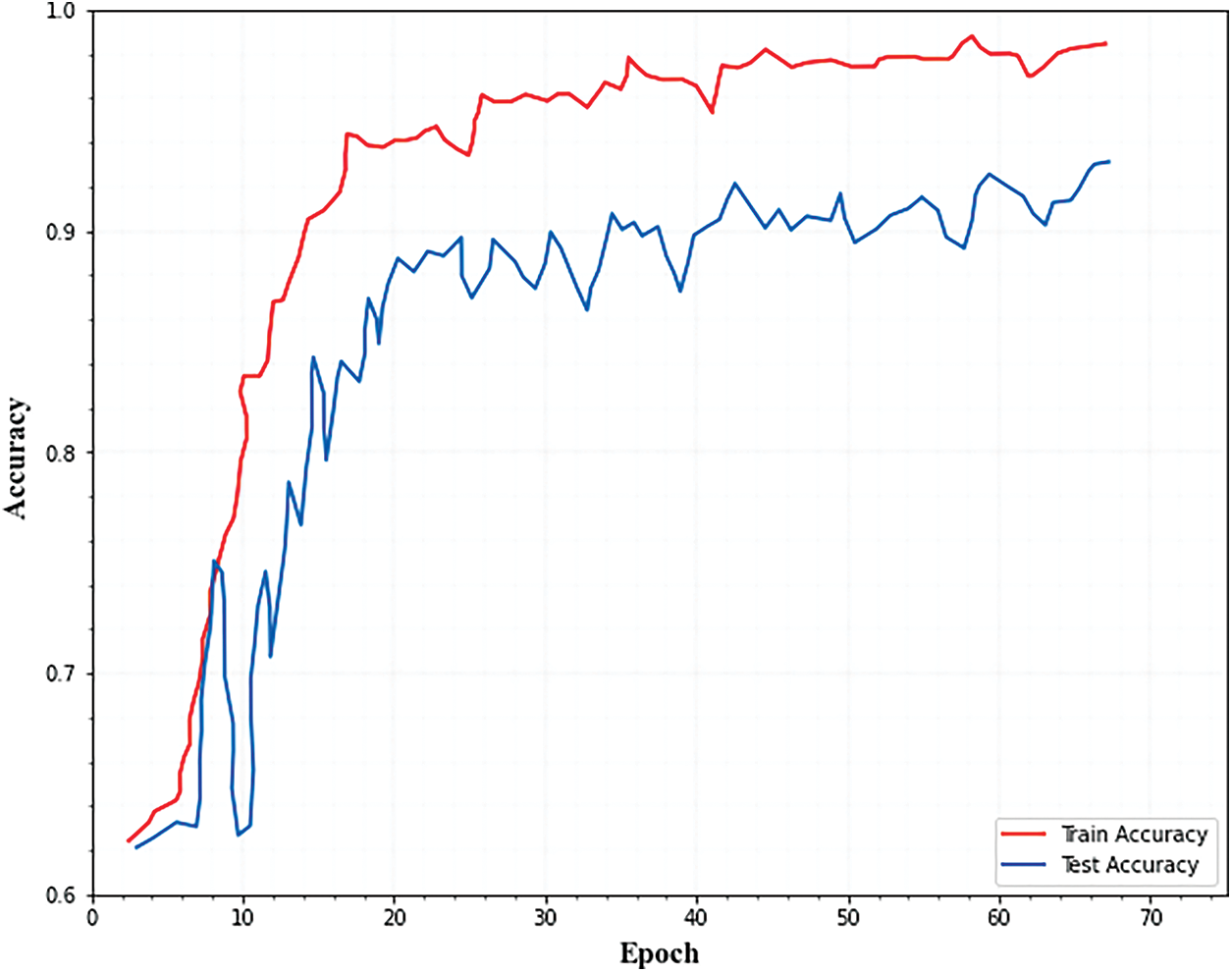
Figure 2: Training and testing accuracy for classification

Both training and testing losses must be kept to a minimum. If the testing loss is greater than the training loss, the network is overfitting. Overfitting can be reduced by using the optimization technique to increase each fractal block’s dropout. Fig. 3. Illustrates that as the number of epochs increased, the training and testing errors decreased.

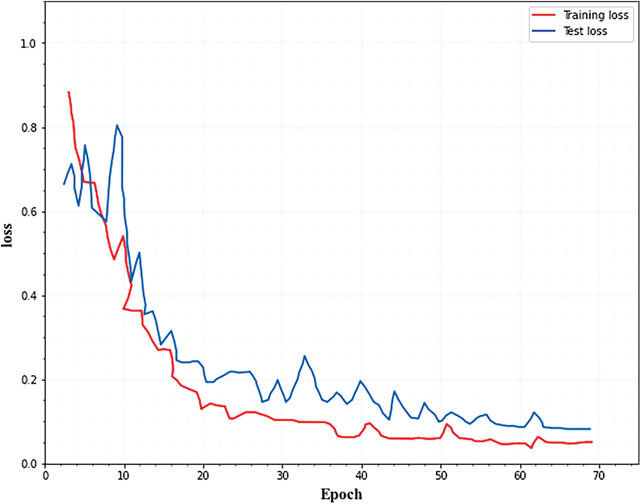
Figure 3: Training and testing loss for classification

Figs. 4 and 5. show the accuracy and loss curves of the segmentation network. From the figures, it is observed that the loss curve converges after 40 epochs and the accuracy curve converges after 20 epochs.

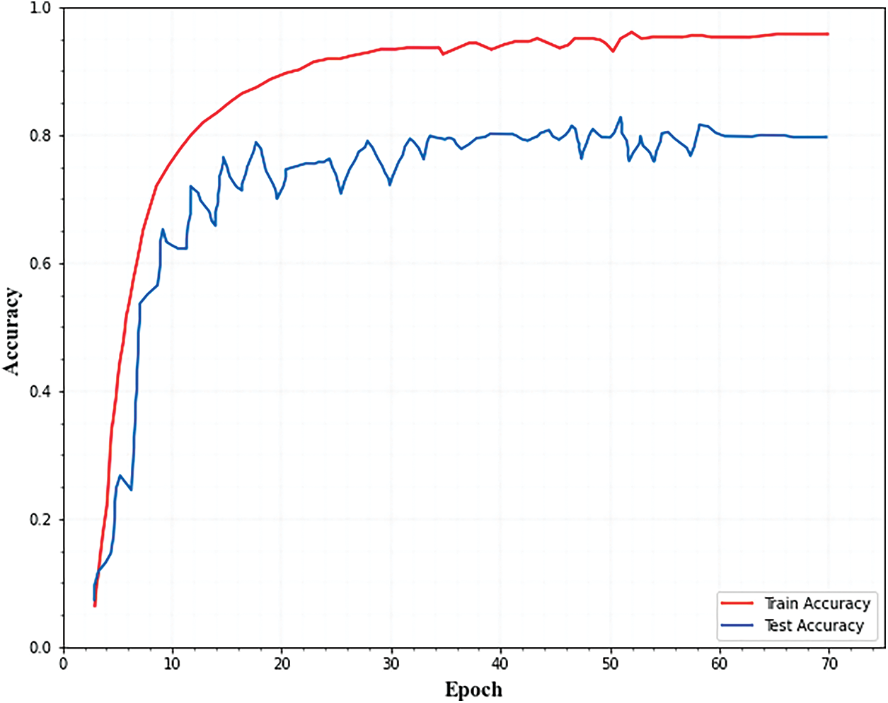
Figure 4: Training and testing accuracy for segmentation

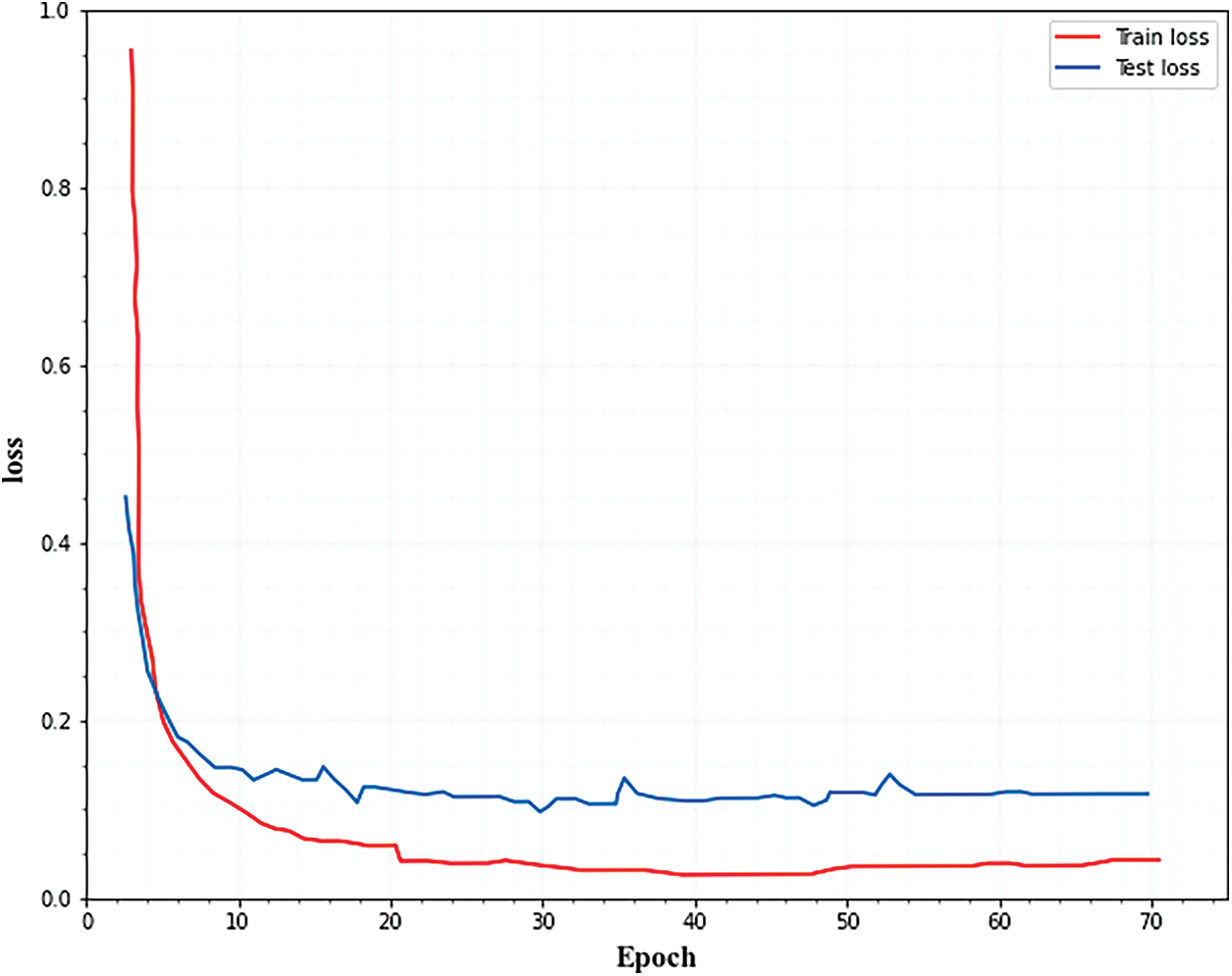
Figure 5: Training and testing loss for segmentation

5.3 Segmentation Results

In this section, the segmentation performance of the proposed approach is evaluated and results are presented. Three variables were derived to assess segmentation performance. They are positive predicted value (PPV), sensitivity (SEN_S), and dice similarity coefficient (DSC). The Dice coefficient was used to evaluate the accuracy of the segmentation algorithm that measured the similarity of two samples. The PPV represents the proportion of all correctly segmented patellar dislocation points in the predicted patellar dislocation points and SEN_S represents the proportion of correctly segmented images to the real image which are defined as follows,

DSC=2TPVFPV+FNV+2TPV(22)

PPV=TPVTPV+FPV(23)

SEN_S =TPVTPV+FNV(24)

Here, True positive pixels denote TPV, False positive pixels denote FPV and the amount of false negative pixels denotes FNV. The ratio of true positive pixels to false negative pixels is denoted as sensitive (SEN_S).

The segmented images of the brain tissues and the comparison among the ground truth images are given in Fig. 6. From the segmented images, it is revealed that the margins between the grey and white matter are much more distinct, bold, and contrast-enhancing. The hippocampus area boundary is additionally apparent. In conclusion, the suggested method shows that it is efficient at extracting meaningful edge points from brain MRI data. As a result, it is possible to identify the stages of Alzheimer’s disease with greater accuracy.

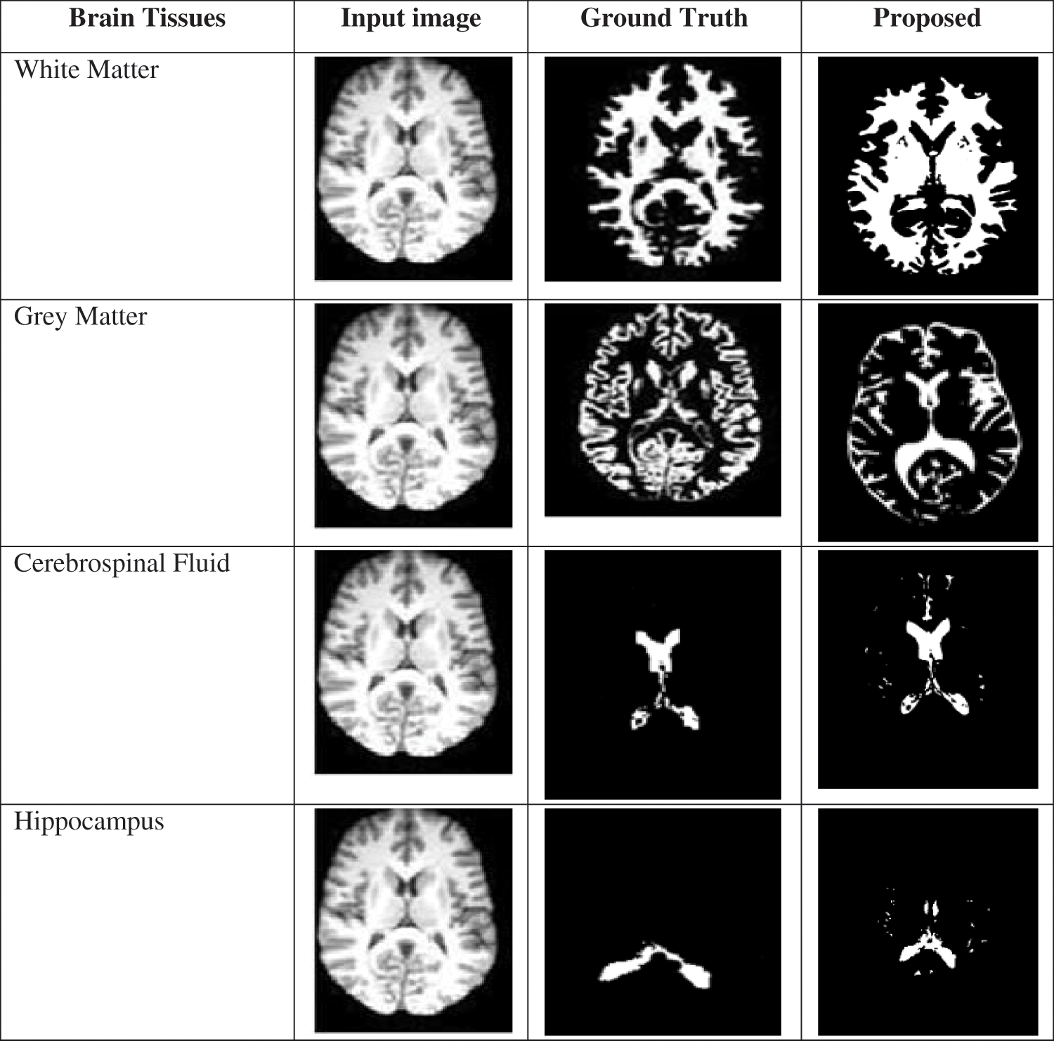
Figure 6: Comparison of a proposed segmented image with ground truth

The calculated results of the three assessment indexes come closer to showing superior segmentation effects. The quantitative results of the segmentation technique are shown in Table 1. From Table 1 it is observed that the LMCI class achieves high DSC and SEN_s. The AD and EMCI classes also achieve good performance. The graphical representation of this Table 1 is given in Fig. 7.

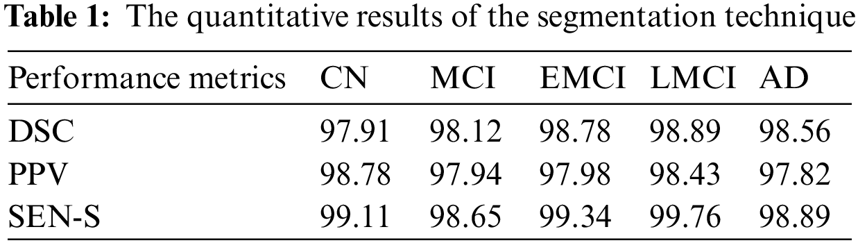
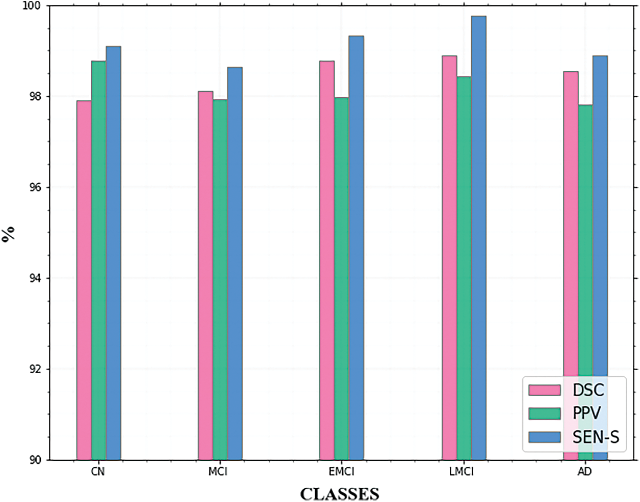
Figure 7: Comparison of segmentation metrics for AD classes

For the suggested approach, detailed assessments show that the proposed method demonstrated its superiority in detecting significant object boundaries from brain MRI data. As a result, the phases of Alzheimer’s disease can be detected more precisely.

The suggested segmentation approach was compared to existing approaches in Table 2. When comparing the quantitative results of the various approaches listed in Table 2, it could be seen that the validation of the suggested system produced good results for brain segmentation. Using the proposed method, we achieve a DSC of 98.45%, a PPV of 98.19%, and a Sensitivity of 99.15%. The graphical representation of the DSC metric comparison is given in Fig. 8.

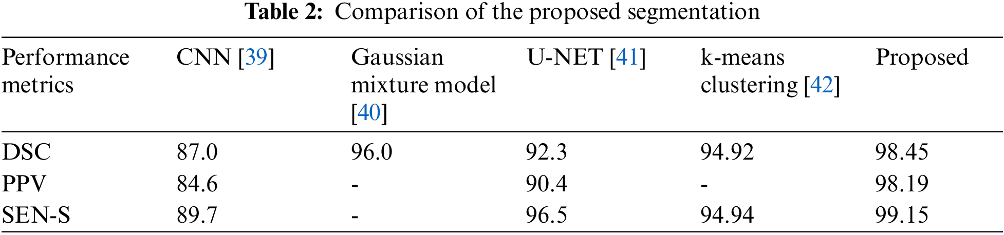
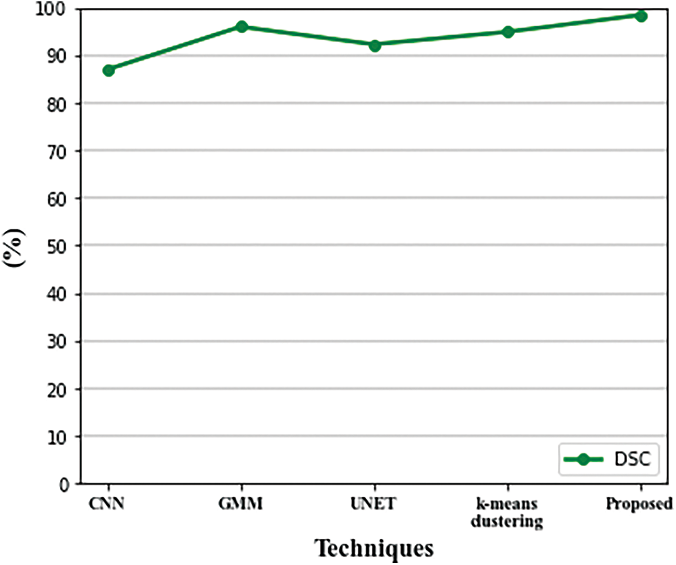
Figure 8: Comparison of DSC metric with existing techniques

5.4 Classification Results

This section presents the multi-class classification results of the proposed approach and its comparison with the existing techniques to find out the effectiveness of the method. The purpose of the model evaluation is to help decide how well a given data model generalizes to new data so that we can distinguish between different models. To this end, we need a metric calculation to determine the performance of various models. The performance metrics used for classification are shown in the following equation.

A basic metric is classification accuracy, which calculates how much an instance class is correctly predicted by the model in the validation set.

Accuracy=TP+TNTP+TN+FP+FN(25)

The Recall indicates the classifier’s ability to locate all positive samples.

Recall=TPTP+FN(26)

The positive prediction’s proportion is called precision as stated in the following equation,

Precision=TP+TNTP+FP(27)

The curve formed by comparing the True Positive Rate (TPR) vs. False Positive Rate (FPR) is known as the receiver operating characteristic (ROC) curve.

TPR=TPTP+FN,FPR=FPFP+TN

In estimating classification performance, the AUC is a key metric.

Table 3 summarizes the outcomes of our evaluation and Fig. 9. illustrates the graphical representation of the five class’s outcomes. The confusion matrix of the proposed approach is shown in Fig. 10. In the confusion matrix, the main diagonal contains major values. It means the majority of the images are correctly classified by the proposed approach.

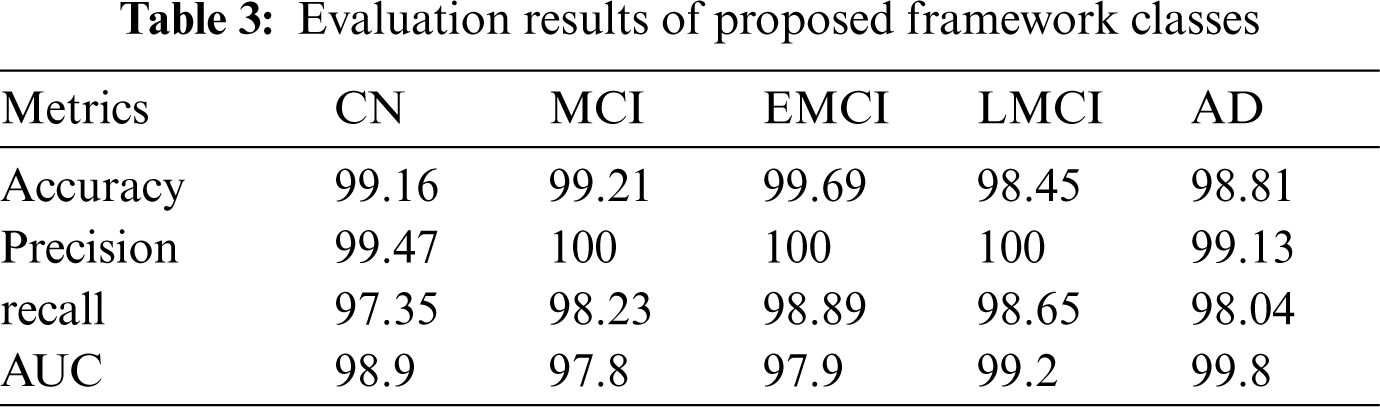
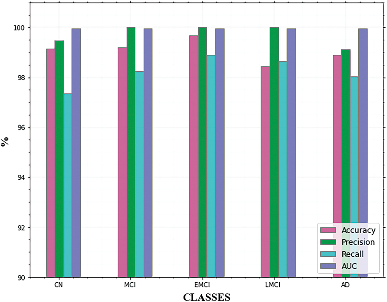
Figure 9: Comparison of AD classes

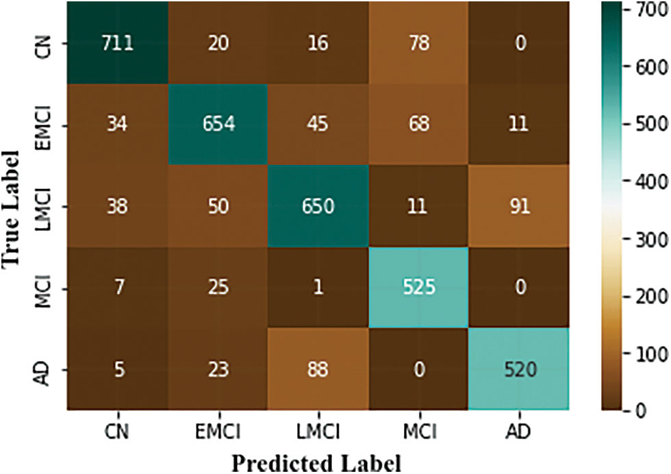
Figure 10: Confusion matrix of the proposed approach

These subcategories were utilized to identify the phases of AD. Each of the classes has features that show the existence of AD, although in varying degrees depending on the subclasses’ dimensions. Fig. 11. shows the ROC curves for these classes.

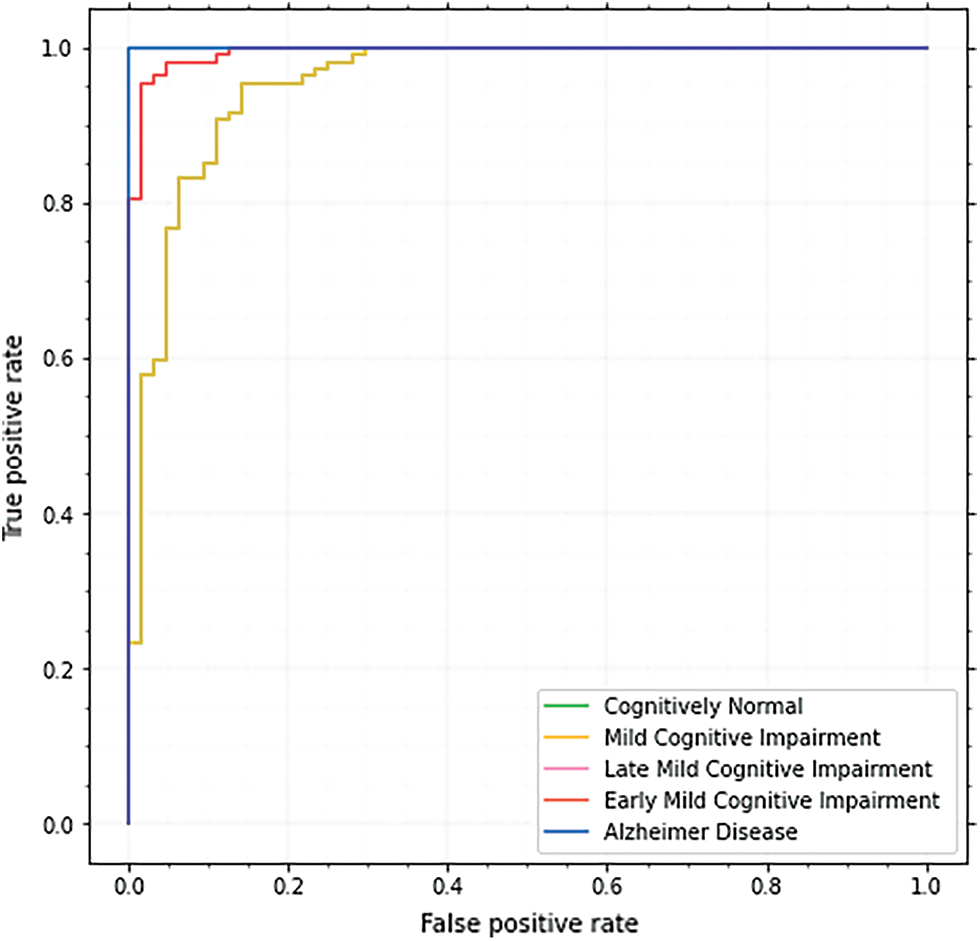
Figure 11: ROC curve of the proposed approach

Each model’s ROC curve is used to examine the classifier and is recognized as a valuable tool. For CN, MCI, EMCI, LMCI, and AD, the ROC curve is 98.9, 97.8, 97.9, 99.2, and 99.8 respectively. The AUC score for AD is the highest, although other classes also do well.

From Table 4, it is observed that the deep separable convolutional neural network (DSCNN) attained the lowest accuracy for classification accuracy at 75.32%. The accuracy of CNN, Dementia Network (DEMENT), and Resnet-101 seemed better than DSCNN but not as good as fractalnet. The accuracy and recall of Resnet were 96.3% and 96.7% correspondingly. But the training time of resnet was higher which increased the time complexity of the network. Although the FCN achieved good results, during the feature extraction process, loss of details was often caused by repeated subsampling and excessive sampling frequencies. The alexnet attained higher accuracy and recall value than 3DCNN. But it had a very shallow depth which made it difficult to learn features from larger images. From all the above discussions, it is observed that the proposed approach provides superior performance than other techniques in terms of all metrics with its efficient handling of complex tasks.

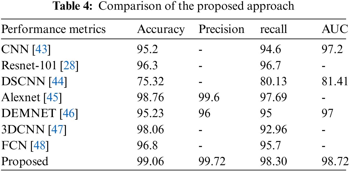
In terms of recall, Alexnet attained good performance, and Dementia and FCN provided similar results. The accuracy, precision, and recall of fractalnet were better than the other four techniques. Although alexnet’s accuracy was 98.76% which is similar to fractalnet. Even though fractalnet was superior to alexnet in terms of all metrics. The graphical representation of accuracy and recall comparison is given in Fig. 12.

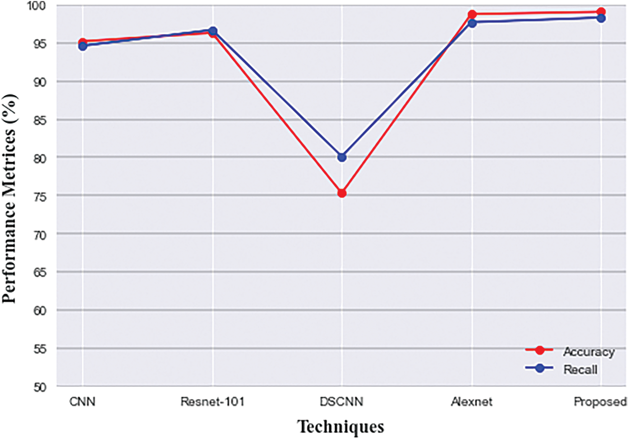
Figure 12: Comparison of accuracy and recall of proposed with existing techniques

5.5 Statistical Analysis

To examine the statistical significance of observed performance results, we used a one-way ANOVA test for which the results are displayed in Table 5. The significance level for the test was set to α = 0.05. F-value, mean, and p-value are statistical analysis results for multiple comparisons.

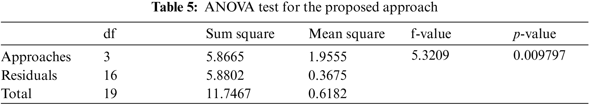
Significant levels are determined by P < 0.05. The group variation rate is denoted by the F-value which is the ratio of mean squares within groups to mean squares between groups. Inverse proportionality exists between P and F values. P-value equals 0.00979738, [p (x ≤ F) = 0.990203]. It means that the chance of type1 error is small (0.98%). The observed effect size f is large (1). That indicates that the magnitude of the difference between the averages is large. The η2 equals 0.5. It means that the group explains 49.9% of the variance from the average. From all the above observations, it is understood that the proposed framework provides the best performance to classify AD which is helpful for the medical sector.

6  Limitations and Future Scope

The suggested method performs well in the segmentation and classification of AD, however, there are still a few issues that should be further considered in future studies. First, there are several redundant or irrelevant features are extracted during the feature extraction process. It may reduce the performance of the classifier. Therefore, an effective feature selection technique is required for this framework to select significant features from the feature set. Second, the proposed approach used only MRI image modalities. Other image modalities contain various types of features. Therefore, the enhancement of the proposed framework is needed to handle various types of image modalities. Third, in this work, only five classes of AD are detected. Therefore, the analysis can be performed for various other phases of AD, such as progressive MCI, stable MCI, etc. This could aid in the initial diagnosis of AD. Moreover, the time complexity of the proposed approach is a little high attributing to the nested connections and the interconnection between the nodes in unet++ and fractalnet which a little more time to produce the results. In the future, specific modifications need to be made to this framework to reduce the time complexity.

7  Conclusion

AD is a serious neurological syndrome that affects a large portion of the global population. Early detection of AD is essential to improve the quality of people’s lives and the development of better treatments with specialized medicines. The proposed framework was established to show the effectiveness of the deep learning algorithms to perform multi-class classification of AD and its various stages like LMCI, EMCI, MCI, CN, and AD. Experiments on the ADNI dataset are used to examine the proposed method in depth. Furthermore, the findings of the proposed approach are compared with the existing methods and the experimental findings show that the model exceeds the competition and achieves an accuracy rate of 99.06%.

Funding Statement: The authors received no specific funding for this study.

Conflicts of Interest: The authors declare that they have no conflicts of interest to report regarding the present study.

References

 1.  X. Zhou, S. Qiu, P. S. Joshi, C. Xue, R. J. Killiany et al., “Enhancing magnetic resonance imaging-driven. Alzheimer’s disease classification performance using generative adversarial learning,” Alzheimer’s Research & Therapy, vol. 13, no. 1, pp. 1–11, 2021. [Google Scholar]

 2.  R. Ferri, C. Babiloni, V. Karami, A. I. Triggiani, F. Carducci et al., “Stacked autoencoders as new models for an accurate Alzheimer’s disease classification support using resting-state EEG and MRI measurements,” Clinical Neurophysiology, vol. 132, no. 1, pp. 232–245, 2021. [Google Scholar]

 3.  R. Divya and R. Shantha Selva Kumari, “Genetic algorithm with logistic regression feature selection for Alzheimer’s disease classification,” Neural Computing and Applications, vol. 33, no. 14, pp. 8435–8444, 2021. [Google Scholar]

 4.  S. Alinsaif and J. Lang, “Alzheimer’s disease neuroimaging initiative: 3D shearlet-based descriptors combined with deep features for the classification of Alzheimer’s disease based on MRI data,” Computers in Biology and Medicine, vol. 138, no. 3, pp. 104879, 2021. [Google Scholar]

 5.  M. S. N. Raju and B. S. Rao, “Colorectal multi-class image classification using deep learning models,” Bulletin of Electrical Engineering and Informatics, vol. 11, no. 1, pp. 195–200, 2022. [Google Scholar]

 6.  E. Hossain, M. S. Hossain, S. Al Jannat, M. Huda, S. Alsharif et al., “Brain tumor auto-segmentation on multimodal imaging modalities using deep neural network,” Computers Materials & Continua, vol. 72, no. 3, pp. 4509–4523, 2022. [Google Scholar]

 7.  S. P. K. Reddy and G. Kandasamy, “Cusp pixel labeling model for objects outline using R-CNN,” IEEE Access, vol. 10, no. 2, pp. 8883–8890, 2021. [Google Scholar]

 8.  Y. Liang, G. Xu and S. U. Rehman, “Multi-scale attention-based deep neural network for brain disease diagnosis,” Computers Materials & Continua, vol. 72, no. 3, pp. 4645–4661, 2022. [Google Scholar]

 9.  H. A. Helaly, M. Badawy and A. Y. Haikal, “Toward deep mri segmentation for Alzheimer’s disease detection,” Neural Computing and Applications, vol. 34, no. 2, pp. 1047–1063, 2022. [Google Scholar]

10. E. Balboni, L. Nocetti, C. Carbone, N. Dinsdale, M. Genovese et al., “The impact of transfer learning on 3D deep learning convolutional neural network segmentation of the hippocampus in mild cognitive impairment and Alzheimer disease subjects,” Human Brain Mapping, vol. 43, no. 11, pp. 3427–3438, 2022. [Google Scholar]

11. N. P. Ansingkar, R. Patil and P. D. Deshmukh, “An efficient multi-class Alzheimer detection using hybrid equilibrium optimizer with capsule auto encoder,” Multimedia Tools and Applications, vol. 81, no. 1, pp. 6539–6570, 2022. [Google Scholar]

12. S. Prabha, K. Sakthidasan, Sankaran and D. Chitradevi, “Efficient optimization based thresholding technique for analysis of Alzheimer MRIs,” International Journal of Neuroscience, vol. 14, no. 3, pp. 1–14, 2021. [Google Scholar]

13. H. Allioui, M. Sadgal and A. Elfazziki, “Intelligent environment for advanced brain imaging: A multi-agent system for an automated Alzheimer diagnosis,” Evolutionary Intelligence, vol. 14, no. 4, pp. 1523–1538, 2021. [Google Scholar]

14. H. Nawaz, M. Maqsood, S. Afzal, F. Aadil, I. Mehmood et al., “A deep feature-based real-time system for Alzheimer disease stage detection,” Multimedia Tools and Applications, vol. 80, no. 28, pp. 35789–35807, 2021. [Google Scholar]

15. G. Mirzaei and H. Adeli, “Machine learning techniques for the diagnosis of Alzheimer’s disease, mild cognitive disorder, and other types of dementia,” Biomedical Signal Processing and Control, vol. 72, no. 1, pp. 103293, 2022. [Google Scholar]

16. J. V. Shanmugam, B. Duraisamy, B. C. Simon and P. Bhaskaran, “Alzheimer’s disease classification using pre-trained deep networks,” Biomedical Signal Processing and Control, vol. 71, no. 2, pp. 103217, 2022. [Google Scholar]

17. N. Goenka and S. Tiwari, “AlzVNet: A volumetric convolutional neural network for multi-class classification of Alzheimer’s disease through multiple neuroimaging computational approaches,” Biomedical Signal Processing and Control, vol. 74, no. 1, pp. 103500, 2022. [Google Scholar]

18. Y. Eroglu, M. Yildirim and A. Cinar, “mRMR-based hybrid convolutional neural network model for classification of Alzheimer’s disease on brain magnetic resonance images,” International Journal of Imaging Systems and Technology, vol. 32, no. 2, pp. 517–527, 2022. [Google Scholar]

19. R. Divya and R. Shantha Selva Kumari, “Genetic algorithm with logistic regression feature selection for Alzheimer’s disease classification,” Neural Computing and Applications, vol. 33, no. 14, pp. 8435–8444, 2021. [Google Scholar]

20. S. Nagaraj and T. Q. Duong, “Deep learning and risk score classification of mild cognitive impairment and Alzheimer’s disease,” Journal of Alzheimer’s Disease, vol. 80, no. 3, pp. 1079–1090, 2021. [Google Scholar]

21. X. Zhou, S. Qiu, P. S. Joshi, C. Xue, R. J. Killiany et al., “Enhancing magnetic resonance imaging-driven Alzheimer’s disease classification performance using generative adversarial learning,” Alzheimer’s Research & Therapy, vol. 13, no. 1, pp. 1–11, 2021. [Google Scholar]

22. R. R. Janghel and Y. K. Rathore, “Deep convolution neural network based system for early diagnosis of Alzheimer’s disease,” IRBM, vol. 42, no. 4, pp. 258–267, 2021. [Google Scholar]

23. S. Murugan, C. Venkatesan, M. G. Sumithra, X. Z. Gao, B. Elakkiya et al., “DEMNET: A deep learning model for early diagnosis of Alzheimer diseases and dementia from MR images,” IEEE Access, vol. 9, no. 1, pp. 90319–90329, 2021. [Google Scholar]

24. X. Gao, F. Shi, D. Shen and M. Liu, “Task-induced pyramid and attention gan for multimodal brain image imputation and classification in Alzheimer’s disease,” IEEE Journal of Biomedical and Health Informatics, vol. 26, no. 1, pp. 36–43, 2021. [Google Scholar]

25. M. Li, C. Hu, Z. Liu and Y. Zhou, “MRI segmentation of brain tissue and course classification in Alzheimer’s disease,” Electronics, vol. 11, no. 8, pp. 1288, 2022. [Google Scholar]

26. R. Basnet, M. O. Ahmad and M. N. S. Swamy, “A deep dense residual network with reduced parameters for volumetric brain tissue segmentation from MR images,” Biomedical Signal Processing and Control, vol. 70, no. 1, pp. 103063, 2021. [Google Scholar]

27. J. S. Long, G. Z. Ma, E. M. Song and R. C. Jin, “Learning u-net based multi-scale features in encoding-decoding for MR image brain tissue segmentation,” Sensors, vol. 21, no. 9, pp. 3232, 2021. [Google Scholar]

28. P. R. Buvaneswari and R. Gayathri, “Deep learning-based segmentation in the classification of Alzheimer’s disease,” Arabian Journal for Science and Engineering, vol. 46, no. 6, pp. 5373–5383, 2021. [Google Scholar]

29. Z. Xu, H. Deng, J. Liu and Y. Yang, “Diagnosis of Alzheimer’s disease based on the modified tresnet,” Electronics, vol. 10, no. 16, pp. 1908, 2021. [Google Scholar]

30. S. Basheera and M. S. S. Ram, “Deep learning based Alzheimer’s disease early diagnosis using T2w segmented gray matter MRI,” International Journal of Imaging Systems and Technology, vol. 31, no. 3, pp. 1692–1710, 2021. [Google Scholar]

31. Y. AbdulAzeem, W. M. Bahgat and M. Badawy, “A CNN based framework for classification of Alzheimer’s disease,” Neural Computing and Applications, vol. 33, no. 16, pp. 10415–10428, 2021. [Google Scholar]

32. R. E. Turkson, H. Qu, C. B. Mawuli and M. J. Eghan, “Classification of Alzheimer’s disease using deep convolutional spiking neural network,” Neural Processing Letters, vol. 53, no. 4, pp. 2649–2663, 2021. [Google Scholar]

33. M. Amini, M. Pedram, A. Moradi and M. Ouchani, “Diagnosis of Alzheimer’s disease severity with fMRI images using robust multitask feature extraction method and convolutional neural network (CNN),” Computational and Mathematical Methods in Medicine, vol. 2021, no. 3, pp. 5514839, 2021. [Google Scholar]

34. M. H. Al-Adhaileh, “Diagnosis and classification of Alzheimer’s disease by using a convolution neural network algorithm,” Soft Computing, vol. 26, no. 1, pp. 7751–7762, 2022. [Google Scholar]

35. C. Srinivas, N. P. KS, M. Zakariah, Y. A. Alothaibi, K. Shaukat et al., “Deep transfer learning approaches in performance analysis of brain tumor classification using MRI images,” Journal of Healthcare Engineering, vol. 2022, no. 2, pp. 3264367, 2022. [Google Scholar]

36. X. Yang, M. Khushi and K. Shaukat, “Biomarker CA125 feature engineering and class imbalance learning improve ovarian cancer prediction,” in 2020 IEEE Asia-Pacific Conf. on Computer Science and Data Engineering (CSDE), Gold Coast, Australia, IEEE, pp. 1–6, 2020. [Google Scholar]

37. T. M. Alam, K. Shaukat, A. Khelifi, H. Aljuaid, M. Shafqat et al., “A fuzzy inference-based decision support system for disease diagnosis,” The Computer Journal, vol. 2022, no. 1, pp. bxac068, 2022. [Google Scholar]

38. L. Devnath, P. Summons, S. Luo, D. Wang, K. Shaukat et al., “Computer-aided diagnosis of coal workers’ pneumoconiosis in chest x-ray radiographs using machine learning: A systematic literature review,” International Journal of Environmental Research and Public Health, vol. 19, no. 11, pp. 6439, 2022. [Google Scholar]

39. M. Liu, F. Li, H. Yan, K. Wang, Y. Ma, et al., “Alzheimer’s disease neuroimaging initiative: A multi-model deep convolutional neural network for automatic hippocampus segmentation and classification in Alzheimer’s disease,” Neuroimage, vol. 208, no. 3, pp. 116459, 2020. [Google Scholar]

40. A. T. Tuan, T. B. Pham, J. Y. Kim and J. M. R. Tavares, “Alzheimer’s diagnosis using deep learning in segmenting and classifying 3D brain MR images,” International Journal of Neuroscience, vol. 132, no. 7, pp. 1–10, 2020. [Google Scholar]

41. H. Yousefi-Banaem and S. Malekzadeh, “Hippocampus segmentation in magnetic resonance images of Alzheimer’s patients using deep machine learning,” arXiv Preprint, vol. 109, no. 1, pp. 67–79, 2021. [Google Scholar]

42. Z. S. Aaraji and H. H. Abbas, “Automatic classification of Alzheimer’s disease using brain MRI data and deep convolutional neural networks,” arXiv Preprint, vol. 109, no. 3, pp. 159–185, 2022. [Google Scholar]

43. S. Basheera and M. S. S. Ram, “A novel CNN based Alzheimer’s disease classification using hybrid enhanced ICA segmented gray matter of MRI,” Computerized Medical Imaging and Graphics, vol. 81, no. 1, pp. 101713, 2020. [Google Scholar]

44. J. Liu, M. Li, Y. Luo, S. Yang, W. Li et al. “Alzheimer’s disease detection using depthwise separable convolutional neural networks,” Computer Methods and Programs in Biomedicine, vol. 203, no. 1, pp. 106032, 2021. [Google Scholar]

45. B. Lee, W. Ellahi and J. Y. Choi, “Using deep CNN with data permutation scheme for classification of Alzheimer’s disease in structural magnetic resonance imaging (sMRI),” IEICE TRANSACTIONS on Information and Systems, vol. 102, no. 7, pp. 1384–1395, 2019. [Google Scholar]

46. S. Murugan, C. Venkatesan, M. G. Sumithra, X. Z. Gao, B. Elakkiya et al., “DEMNET: A deep learning model for early diagnosis of Alzheimer diseases and dementia from MR images,” IEEE Access, vol. 9, no. 3, pp. 90319–90329, 2021. [Google Scholar]

47. E. Goceri, “Diagnosis of Alzheimer’s disease with sobolev gradient-based optimization and 3D convolutional neural network,” International Journal for Numerical Methods in Biomedical Engineering, vol. 35, no. 7, pp. e3225, 2019. [Google Scholar]

48. S. Qiu, P. S. Joshi, M. I. Miller, C. Xue, X. Zhou et al., “Development and validation of an interpretable deep learning framework for Alzheimer’s disease classification,” Brain, vol. 143, no. 6, pp. 1920–1933, 2020. [Google Scholar]

Appendix-1