Hybrid Feature Selection Method for Predicting Alzheimer’s Disease Using Gene Expression Data

1  Introduction

Dementia and memory loss are commonly caused by AD. It seems that in the mid of 1906, AD is first recognized. It has been discovered as the principal reason for death. AD begins slowly and slowly exacerbates over time [1]. By 2050, approximately 152 million people worldwide will be detected with AD [2]. It is expected that [3] one person out of every eighty-five will suffer from AD by 2050. AD has various symptoms; the most prevalent is the inability of remembering recent occurrences. Difficulties with self-motivation, language, orientation, memory, self-care, mood, and behavior are some indications of advanced AD [4]. As the status of AD patients degenerates, they start to keep away from their families and society. Progressively, Body functions are lost, which finally results in death. Despite progress might happen quickly or slowly, the average life expectancy after an AD diagnosis is 3 to 9 years [5]. As a result, early identification of AD has the potential to save lives, which is where the current research comes into play.

So far, most of the recent studies on AD diagnosis have been performed using neuropsychological testing and brain magnetic resonance imaging (MRI). Because it was challenging to sample the posterior brains of normal and AD individuals, molecular recognition of AD is inadequate. Recent trials have thankfully yielded large-scale omics data for numerous brain locations. Using this data, it is now quite simple to construct prediction approaches, like those described in this study, in which ML techniques are used to diagnose AD earliest opportunity. These treatments can be advantageous for the patient because they are simple and affordable. In certain cases, they have even been demonstrated to predict AD better than physicians [6]. This fact has prompted a lot of studies into utilizing ML to diagnose AD using medical data in various ways, such as MRI.

In the following articles, the authors used MRI in the diagnosis of AD: an approach based on SVM with recursive feature elimination to choose the informative features is employed in [7]. They allegate to have better performance in classifying normal (N), mild cognitive impairment (MCI), and AD cases (subjects or instances). The authors in [8] used MRI images with an unsupervised convolutional neural network (CNN) for AD feature extraction. In addition, they classify AD, MCI, and N by employing k-means clustering. The output achieves an accuracy of 95.52% for AD vs. MCI and 90.63% for MCI vs. N in one slice of data. For TOP data, the method achieves an accuracy of 97.01% for AD vs. MCI, and an accuracy of 92.6% for MCI vs. N. Techniques of the type Resting-state functional MRI and deep learning (DL) have been used in [9] to classify AD and its stages. To apply transfer learning with and without fine-tuning, they used an expanded network architecture. While off-the-shelf and fine-tuned models, they produce impressive outcomes with high accuracy. The study in [10] classified AD and MCI cases from N cases using CNN. They investigate the effects of including information from diffusion tensor imaging and MRI. They achieved AUC, specificity, and Acc results of 0.93%, 91.7%, and 88.9%, respectively, for N vs. AD classification, and 0.68%, 81.8%, and 71.1%, respectively, for N vs. MCI classification.

Interesting results have been obtained in [11], where MRI is used to classify stable MCI, converter MCI, N, and AD cases. For dimensionality reduction, they used partial least squares and Analysis of variance (ANOVA) for features selection. For classification, random forest (RF) is used, obtaining an accuracy of 56.25% for a test set of 160 cases. In [12], mobility data and DL models are used to identify the stage of AD patients by processing a time series for each patient. In addition, a CNN model is used to identify the patterns which detect AD stages. The results outperform those of traditional supervised learning models. In [13] the authors used MRI images to check the presence of AD and to assess the degree of AD. An evolutionary algorithm is applied to extract specific information for AD classification. Two experiments are executed; the first one is to classify images into two classes moderate demented and non-demented. The second experiment is to classify images into three classes moderate demented, mild demented, and non-demented. Their approach achieved 100% and 100% for Acc and F1-score, respectively for the first experiment. For the second experiment, they achieved 91.49%, and 91.49% for Acc and F1-score, respectively.

In [14] ML framework is used to automatically diagnose neurodegenerative diseases, focusing on AD and frontotemporal dementia. The authors suggested an explainable artificial intelligence tool to assist clinicians in diagnosis because it includes all the stages necessary to analyze these datasets, including data preparation, feature selection using an evolutionary approach, and modeling of the diseases listed. It was evident how the suggested framework enables fluid processing of the cognitive and image assessments, with a significant decrease in the number of features required for the diagnosis, and a significant increase in classification accuracy.

GE data-based research enables the diagnosis of numerous diseases through the powerful technology of Deoxyribonucleic Acid (DNA) microarrays [15]. Thousands of genes’ expression levels are provided in this data [16]. The gene expression level is signified by some distinct messenger molecules ribonucleic acid (mRNA) in the cell. Utilizing this level, the diseases can be detected and the best treatment options and alterations in other processes can be discovered [17]. In this direction, blood-derived gene expression biomarkers in [18] are used to differentiate AD cases from N cases. XGBoost is used as a classifier and successfully identifies AD by including associated mental and geriatric health issues. However, the model’s sensitivity must be improved to create a more accurate blood test for AD. Three datasets, AD Neuroimaging Initiative (ADNI), AddNeuroMed1 (ANM1), and ANM2 have been used in [19] to classify AD from N. To select the most relevant genes, various GS methods like transcription factor, convergent functional genomics (CFG), hub genes, and variational autoencoder have been employed. Five classifiers, SVM, L1-regularized LR (L1-LR), RF, deep neural network (DNN), and logistic regression (LR) have been implemented for classification purposes. They achieved AUC results as follows 87.4% for ANM1, 80.4% for ANM2, and 65.7% for ADNI. Moreover, the blood genes’ biological functions relevant to AD have been analyzed and the blood bio-signature has been compared with the brain bio-signature. Several 1291 brain genes have been selected from a GE dataset with 2021 blood genes selected from the other datasets, reporting that 140 genes are common among them.

The authors in [20] identify GE from a blood dataset, exploring the correlation between an AD patient’s blood and brain genes. They discover 789 differentially expressed genes in both the brain and blood. The least absolute shrinkage and selection operator (LASSO) regression is utilized as a GS technique. They used logistic ridge regression (RR), RF, and SVM approaches in the classification stage. With 78.1% for Acc, they successfully distinguish AD cases from N cases. To identify prospective diagnostic biomarkers of AD, the authors in [21] used multiple brain regions. GE data from six brain regions are used to identify AD biomarkers. For the selection of the relevant genes, a t-test is employed. To identify biomarkers and gauge their use for clinical diagnosis, Significance tests have been performed. GE and DNA methylation datasets have been integrated in [22] for the prediction of AD using DNN. Moreover, they used t-stochastic nearest neighbor (t-SNE) and principal component analysis (PCA) techniques for gene selection. They verify the effectiveness of their method by comparing its Acc and AUC with those of conventional ML models, like SVM, RF, and Naive Bayes (NB). They achieve 82.3% Acc and 79.7% AUC.

Blood GE data from dementia case registry (DCR) cohorts and the ANM has been used in [23]. For GS, they used recursive feature elimination (RFE) and for the classification task, they used RF. In addition, they used ANM1 for training the classifier and used for testing integration of ANM2 and DCR. Their methods achieve 65.7% for Acc and 72.4% for AUC.

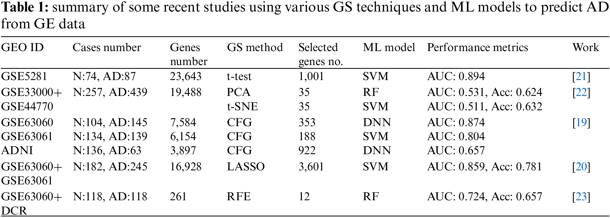
Table 1 presents a summary of recent studies that have been presented to diagnose AD. This table illustrates the main challenge in analyzing GE data: the imbalance between the number of genes and cases (the number of genes is significantly more than the number of cases). The Table lists the number of genes utilized in each experiment at the beginning and after the GS phase. We conclude that the selection of genes is heavily influenced by the dataset and model and doesn’t have any discernible pattern or guideline. In other words, depending on the ML model employed, each experiment may choose a different number for the most significant genes and arrive at a different Acc value.

This paper proposes an approach to predict AD based on GE data, consisting of steps. In the beginning, we preprocess each dataset to prepare the datasets for manipulation. Then, we use a filtering method to evaluate a dataset’s genes. Next, we rank and select the genes that have the highest values. Then we use an embedded method to select the most relevant and significant genes. Finally, we feed the selected genes into various ML techniques and track their classification results. The technique with the greatest performance is chosen to be used in the AD prediction system in the future, which is our ultimate goal.

The structure of the article follows the following order. In Section 2, we present the materials and methods of the approach used in our investigations. Section 3 is devoted to the experimental work. Section 4 is used for the discussion and concluding remarks.

2  Materials and Methods

This section presents our suggested strategy for GS and AD classification as depicted in Fig. 1. Below, we present the details of the suggested strategy.

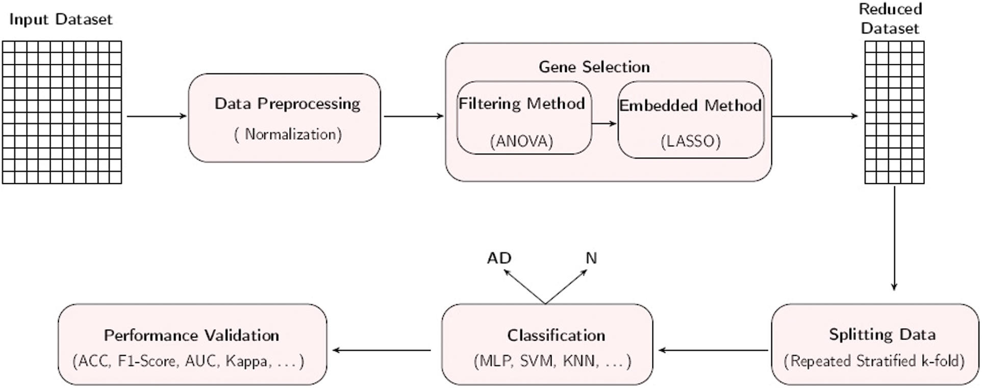
Figure 1: Workflow of the proposed approach for AD prediction

2.1 Datasets

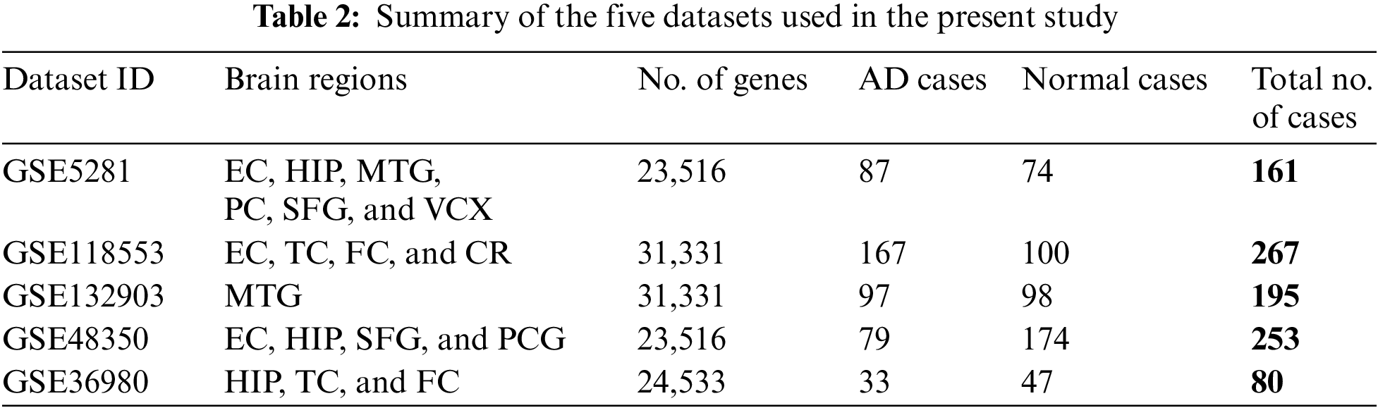
The experimental work is applied using five well-known gene expression datasets. The datasets are composed of multiple human brain tissues for DNA microarray data. They are obtained from the National Center for Biotechnology Information-Gene Expression Omnibus (NCBI-GEO) database [24]. The access numbers of the used datasets are GSE5281, GSE118553, GSE132903, GSE48350, and GSE36980. GSE5281 dataset contains 161 cases from various six brain regions, i.e., medial temporal gyrus (MTG), hippocampus (HIP), entorhinal cortex (EC), primary visual cortex (VCX), superior frontal gyrus (SFG), and posterior cingulate (PC). GSE118553 contains 267 cases from four different brain regions, frontal cortex (FC), temporal cortex (TC), EC, and cerebellum (CR). GSE132903 dataset contains 195 cases from the MTG brain region. GSE48350 dataset contains 253 cases from different four brain regions, i.e., EC, HIP, SFG, and post-central gyrus (PCG). GSE36980 dataset contains 80 cases from three different brain regions HIP, TC, and FC. The five datasets are summarized in Table 2.

2.2 Preprocessing

Preprocessing is essential for handling gene expression data because it prepares the datasets for manipulation. The gene values are normalized to avoid large differences among the genes. The min-max approach is used for normalization, and rescales the values range to the interval [0,1] for each individual gene. Denote by C the set of cases described by G as a set of genes. The normalized gene value Λ^ci,gj, ci∈C, and gj∈G, of some gene value Λci,gj is defined by

Λ^ci,gj=Λci,gj−minck∈C⁡(Λci,gj)maxck∈C⁡(Λci,gj)−minck∈C⁡(Λci,gj)(1)

where minck∈C⁡(Λci,gj) and maxck∈C⁡(Λci,gj) are the minimum and maximum values of gene gj∈G over all cases ck∈C.

2.3 Gene Selection

GS is considered the most challenging task in the gene expression data analysis because compared to the number of genes the number of cases is substantially smaller. Table 2 illustrates this disparity. It’s a crucial step to select genes from the raw gene expression datasets that are relevant to AD prediction. Meanwhile, including insignificant and redundant genes can significantly negatively impact classification accuracy. As a result, we devote great attention to gene selection in our research. There are three forms of gene selection methods: filter, wrapper, and embedded methods. We employ a hybrid method for this phase to take advantage of both the filtering and the embedded methods. Filtering methods are good for a theoretical framework; it helps to understand the structure of the data. It is suitable to be used for larger datasets, as it is fast to be computed. Additionally, the embedded method is also fast and more accurate, considering the interaction of the genes, and is less prone to overfitting. We start by looking at each gene’s importance in AD prediction using a filter-based method, ANOVA, and order the genes according to their ability for AD prediction. Then we select the most relevant and informative genes using an embedded method LASSO. Finally, we assess the importance of genes according to each of the three ML classification techniques that we have used. We can detect the most relevant and essential genes as well as the best accurate technique for predicting AD at the end of these two phases.

•   ANOVA-F statistic:

ANOVA is an efficient tool usually used to gauge the significance of differentiating between the means of two random variables [11]. In the current work, the two variables are a gene and the main output. One metric of the ANOVA family is the F statistic. For a binary dataset with two classes, 1 and 2. We calculate the F statistic of a gene as follows. First, determine the sum of squares and the degrees of freedom, then employ the formula below (see [11]).

F=((ρ1−1)+(ρ2−1))[ρ1(x¯−x¯∗)2+ρ2(x¯−x¯∗∗)2](∑k=1ρ1(x∗,k−x¯∗)2+∑k=1ρ2(x∗∗,k−x¯∗∗)2)(2)

with ρ1 as the number of class 1 cases, and ρ2 as the number of class 2 cases. The overall average of the gene is denoted by x¯, x¯∗ denotes the average of the class 1 gene values, x¯∗∗ is the average of the class 2 gene values, x∗,k the k value, with class 1 gene, and x∗∗,k the average of the values, with class 2 gene. The gene is significant for determining the class, AD or N if the F statistic has a larger value and vice versa.

•   LASSO:

A potent tool with two primary functions: regularization and feature selection. Also known as a form of regression method that uses regularization to best fit a generalized linear model. LASSO shatters the regression coefficient to zero for the variable with the smallest impact on the model, based on the principle of penalizing the regression model (L1-norm). Consequently, the LASSO regression model has the best feature selection ability [25].

ωLasso=argωmin{12∑i=1N(yi−ω0−∑j=1pxijwj)2+λ∑j=1p|wj|}(3)

where λ indicates the penalty parameter, which is frequently obtained using cross-validation, that defines the shrinkage proportion. For instances where the data has a small sample size and a high dimension, like in our case, LASSO maintains a great performance. Additionally, when a small number of variables account for the bulk of the data (have a big coefficient); the remaining variable’s power for prediction is relatively low. Additionally, LASSO has some important benefits, including when features have several collinearities, LASSO effectively addresses this and produces highly independent features. Also, LASSO proved to be computationally less expensive.

2.4 Classification

The classification phase in our approach follows the GS phase, where we identify the most relevant genes to AD prediction. Generally speaking, any ML model can be used to predict AD, but in the experiments below, we’ll focus on the three ML classifiers that proved to be the most effective in this task: MLP, SVM, and k-nearest neighbor (KNN). In the present work, the classification is a binary task, we classify AD cases from N cases. The three classifiers used in our experiment will be described as follows.

•   MLP:

MLP is a feed-forward neural network containing one or more hidden layers that are directed in the following order: input, hidden, and output. The rectified linear unit (ReLU) or sigmoid functions are the activation functions used by MLP. The sigmoid function returns a value in the range [0,1], enabling the neural network to classify the data smartly. However, there is a downside to this sigmoid function feature, i.e., with deeper networks; the function’s output is strongly biased towards the extremes of the range. To overcome this issue, the ReLU function was introduced. It gives 0 for an input value smaller than 0 but remains the original input value if it is larger than 0. The ReLU function is defined by

g(x)=x+≡max(0,x)={0,x<0x,x≥0(4)

where x is the input to a neuron. It is well known that some optimizers that improve and stabilize the learning rates of MLP include momentum, nesterovated gradient, stochastic gradient descent, and adaptive moment estimation (Adam). Adam is applied in our study, because of its low memory needs, great computational efficiency, and scalability with big datasets [26]. Since a learning rate of 0.01 is known to help preventing underfitting, it is the default value for this parameter, which regulates the step size in weight updates.

•   SVM:

SVM is a well-known supervised ML technique that classifies data as follows. First, by nonlinearly transforming the data to higher dimension gene spaces. Second, present a linear optimal hyperplane or a decision boundary to detach the points of different classes (see [27]). SVM seeks to maximize distances between the hyperplane and closest training data points. The SVM classifier (the hyperplane) is denoted by

wT.γ(t)+a=0(5)

w is a weight vector, γ(t) is a nonlinear mapping and a is the bias. The optimal hyperplane is defined by finding w and a which minimize the function

12wT. w+B∑i=1nvi(6)

with some slack variables vi>0, n the number of cases, and B some factor.

•   KNN:

KNN algorithm is a famous nonparametric technique used in regression or classification (see [28]). Based on the inter-sample similarity seen in the training set, KNN intuitively categorizes unlabeled samples. When the number of neighbors is given as a parameter, a small value causes the model’s decision boundary to be complicated and subsequently overfit, whereas a large value causes the decision boundary to be simple and underfit. Consequently, choosing a suitable value for this parameter is crucial. The core parameter of the KNN in this investigation was set to the value demonstrating the maximum performance, n_neighbors, individually for each dataset.

2.5 Performance Metrics

The last phase is to evaluate the performance of the classification techniques. To widen the assessment scope, we used for performance evaluation seven metrics: Acc, F1-score, Kappa index, precision, sensitivity (recall), specificity, and AUC.

To calculate these metrics, we first compose for each classification experiment a confusion matrix, having the number of the cases classified and whether the classification is true or false. Let TP be the number of true positive cases, TN the true negatives, FP the false positives, and FN the false negatives. Then, accuracy is defined as

Acc=TP+TNTP+TN +FP+FN(7)

Note that the denominator represents all Predictions.

The F1-Score is given by

F1{-}score=TPTP+0.5(FP+FN)(8)

Kappa index is given by

Kappa=2×(TP×TN−FN×FP)(TP+FP)×(FP+TN)+(TP+FN)×(FN +TN)(9)

Precision is defined as

Precision=TPTP+FP(10)

Sensitivity (Recall) is denoted by

Sensitivity=TPTP+FN(11)

Specificity is defined as

Specificity=TNTN+FP(12)

3  Experimental Work and Results

This section represents the results of our experimentation to check the validity of the proposed approach. The experiments were carried out using five different datasets consisting of multi-tissue GE profiles from various human brain regions as per the Algorithm below.

All the datasets have the property that the number of genes is significantly more than the number of cases as shown in Table 2. The code was run in Python version 3.7.3 with the Scikit-learn packages, it was executed on an Intel (R) Core (TM) i7-8550U CPU, 8 GB RAM, and 64-bit OS Win 10 configuration. Using this method, the most informative and pertinent genes for AD were chosen, and the other genes that did not contribute to the accuracy of a predictive model or would produce unfavorable outcomes were eliminated. In the beginning, the datasets are preprocessed to facilitate handling GE data. In predicting AD, every gene was evaluated for its relevance using the ANOVA filter metric as mentioned above. Genes are ranked in descending order and we select the highest 1000 genes, these numbers of genes are chosen according to the previous experiment we have done in [29] and achieved great results. Then an embedded method, LASSO, is used to learn which genes best contribute to the model’s accuracy.

Algorithm 1: Best classifier identification and GS using hybrid filter method and embedded method.

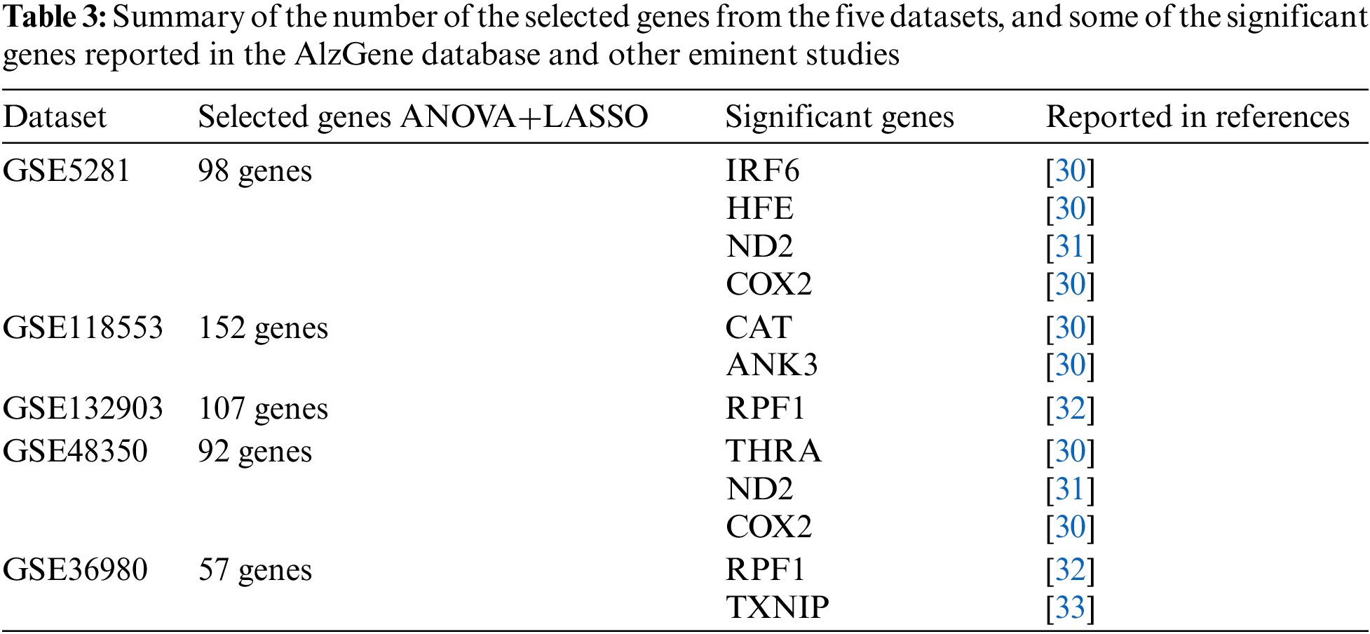
Different numbers of genes are selected from the datasets. These genes are compared with the list of the genes described in the well-known database AlzGene [30], which comprises 695 significant AD genes derived from 1395 research, and other eminent studies. The final number of the selected genes and the most significant genes, which are considered biomarkers of AD, are represented in Table 3. According to the used datasets, we have a kind of imbalanced data, where the number of AD cases is not equal to the normal cases. To overcome such an issue, we split the datasets using a repeated stratified k-fold cross-validation approach, with k = 10 and the number of repetitions is 30 (total of 300 times). This approach is suited for small-sized datasets, which are processed multiple times and report the mean performance across all folds and all repeats. It has the benefit of improving the estimate of the mean model performance.

Every classifier is employed on the selected genes, and the seven performance metrics, (Acc, F1-score, Kappa index, precision, sensitivity (recall), specificity, and the AUC), are evaluated. Finally, the average of 300 results for each performance metric is recorded. We observed that the MLP model achieved the best results in four datasets. In the datasets GSE5281, GSE118553, and GSE132903, MLP contained five hidden layers, each hidden layer consisted of 4 neurons and used the ReLU as the activation function, and Adam as the gradient descent algorithm. The initial learning rate was 0.01 and it is executed over 500 epochs. In GSE48350 datasets MLP contained ten hidden layers and the remaining hyperparameters are the same in the other datasets. SVM achieved the best results in only one dataset, GSE36980. Figs. 2–5 represent the results of our experiment for four metrics, Acc, F1-score, Kappa index, and AUC, whose equations are explained above.

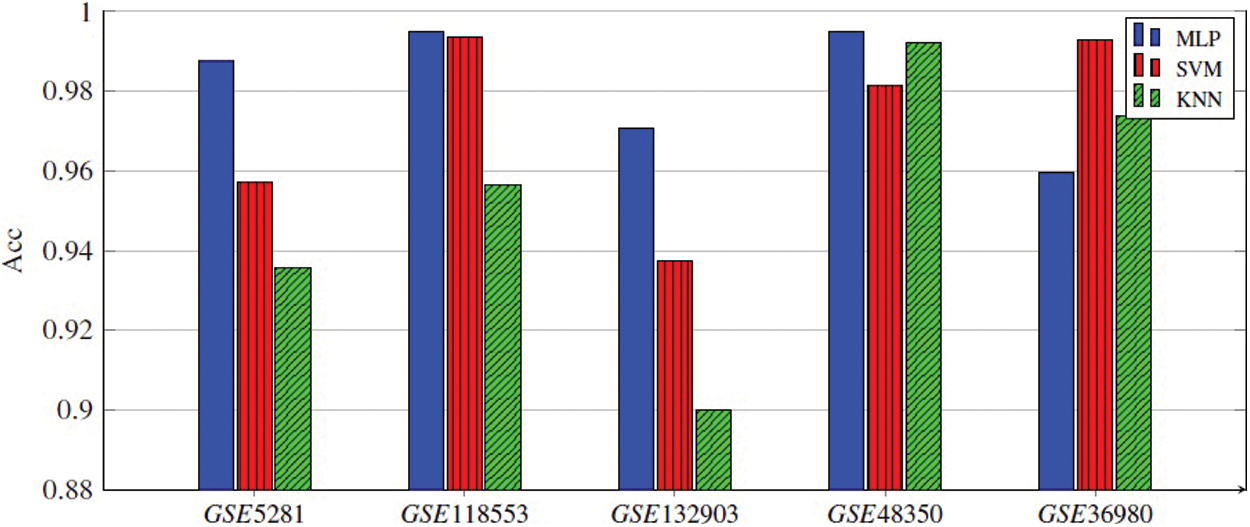
Figure 2: Acc of all three ML models applied for five gene subsets

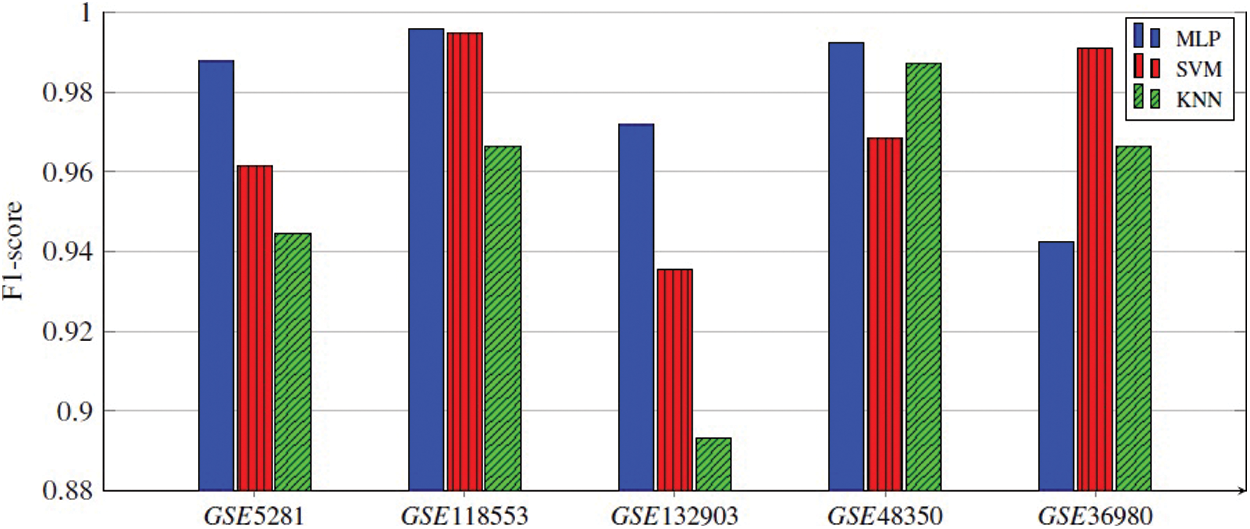
Figure 3: F1-score of all three ML models applied for five gene subsets

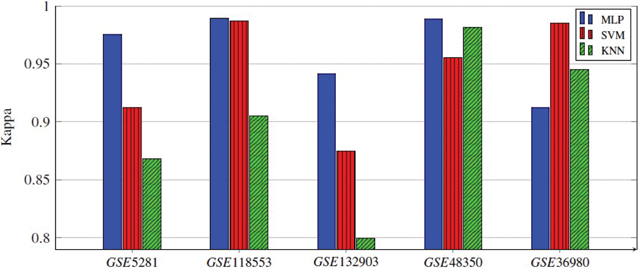
Figure 4: Kappa index of all three ML models applied for five gene subsets

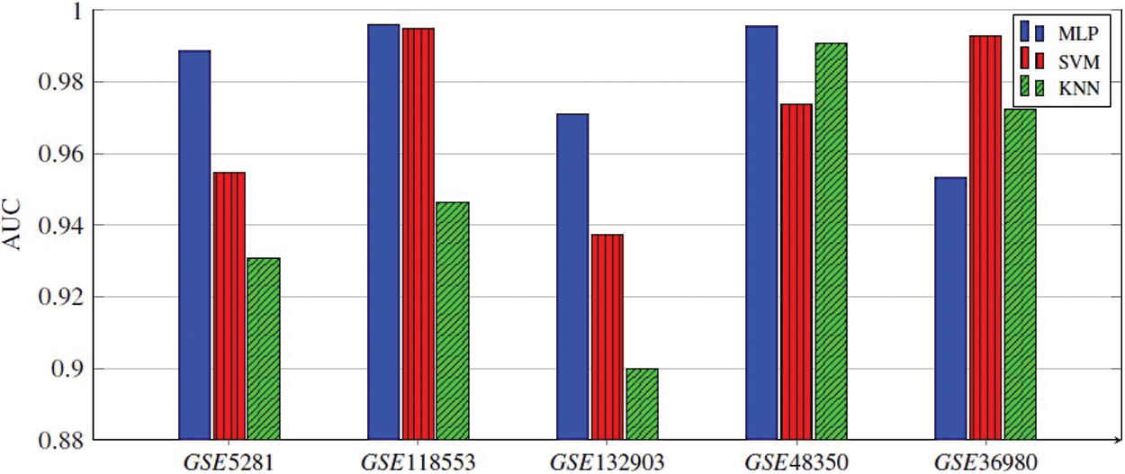
Figure 5: AUC of all three ML models applied for five gene subsets

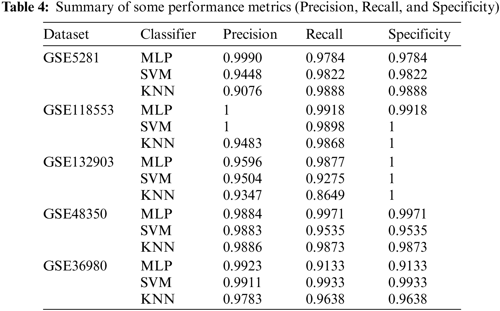
Table 4 represents the average results of the remaining metrics, precision, sensitivity (recall), and specificity. Each figure represents the average values of this metric for three classifiers, MLP, SVM, and KNN, and each selected subset of genes for the five datasets.

4  Conclusion

We presented an approach for predicting a disease that receives insufficient attention in the literature---Alzheimer’s disease, using gene expression data. Compared with recently published competitive approaches, the proposed strategy has been demonstrated to accurately and efficiently predict AD using GE data. We used a hybrid method for GS to decide which genes are most important for AD prediction. In our experiments, five different GE datasets are used. Firstly, we employ a filtering method to rank all the genes according to their importance and select the highest ones. Secondly, we use an embedded method to reduce the number of genes by selecting the most relevant and informative genes. Third, three different classifiers are utilized and the best of them is what achieves the highest performance. It turns out that the MLP model has reached the highest performance and outperforms SVM and KNN in classifying four datasets using the smallest number of genes. While, SVM results outperform MLP and KNN in classifying only one dataset.

The approach is accurate and reliable for classifying AD cases from N cases using the smallest number of genes. Its flexibility characterizes it. It can use any ML classification model, filtering, and embedded method. It can also be applied to other GE-based diseases. It has been proved that it outperforms the state of the art in terms of achieving superior performance with fewer genes. Although the reliability of this work, has one constraint, it is used only for binary classification. Potential future work could solve this constraint by developing a framework capable of predicting AD phases.

Funding Statement: The authors received no specific funding for this study.

Conflicts of Interest: The authors declare that they have no conflicts of interest to report regarding the present study.

References

 1.  M. S. Tan, P. -L. Cheah, A. -V. Chin, L. -M. Looi and S. -W. Chang, “A review on omics-based biomarkers discovery for Alzheimer’s disease from the bioinformatics perspectives: Statistical approach vs machine learning approach,” Computers in Biology and Medicine, vol. 139, no. 2020, pp. 104947, 2021. [Google Scholar]

 2.  F. Chen, J. Bai, S. Zhong, R. Zhang, X. Zhang et al., “Molecular signatures of mitochondrial complexes involved in Alzheimer’s disease via oxidative phosphorylation and retrograde endocannabinoid signaling pathways,” Oxidative Medicine and Cellular Longevity, vol. 2022, no. 4, pp. 1–12, 2022. [Google Scholar]

 3.  S. Wang, P. Phillips, Y. Sui, B. Liu, M. Yang et al., “Classification of Alzheimer’s disease based on eight-layer convolutional neural network with leaky rectified linear unit and max pooling,” Journal of Medical Systems, vol. 42, no. 5, pp. 1–11, 2018. [Google Scholar]

 4.  L. Liu, S. Zhao, H. Chen and A. Wang, “A new machine learning method for identifying Alzheimer’s disease,” Simulation Modelling Practice and Theory, vol. 99, no. 2, pp. 102023, 2019. [Google Scholar]

 5.  W. L. Member, Y. Zhao, X. Chen, Y. Xiao and Y. Qin, “Detecting Alzheimer’s disease on small dataset: A knowledge transfer perspective,” IEEE Journal of Biomedical and Health Informatics, vol. 23, no. 3, pp. 1234–1242, 2018. [Google Scholar]

 6.  S. Alam and G. -R. Kwon, “Alzheimer disease classification using KPCA, LDA, and multi-kernel learning SVM,” International Journal of Imaging Systems and Technology, vol. 27, no. 2, pp. 133–143, 2017. [Google Scholar]

 7.  B. Richhariya, M. Tanveer and A. H. Rashid, “Diagnosis of Alzheimer’s disease using universum support vector machine based recursive feature elimination (USVM-RFE),” Biomedical Signal Processing and Control, vol. 59, pp. 101903, 2020. [Google Scholar]

 8.  X. Bi, S. Li, B. Xiao, Y. Li, G. Wang et al., “Computer aided Alzheimer’s disease diagnosis by an unsupervised deep learning technology,” Neurocomputing, vol. 392, no. 1, pp. 296–304, 2020. [Google Scholar]

 9.  F. Ramzan, M. U. G. Khan, A. Rehmat, S. Iqbal, T. Saba et al., “A deep learning approach for automated diagnosis and multi-class classification of Alzheimer’s disease stages using resting-state fMRI and Residual Neural Networks,” Journal of Medical Systems, vol. 44, no. 2, pp. 37, 2020. [Google Scholar]

10. E. N. M. Id, A. M. Eldeib, I. A. Y. Id and Y. M. Kadah, “Alzheimer’s disease diagnosis from diffusion tensor images using convolutional neural networks,” PLoS One, vol. 15, no. 3, pp. 1–16, 2020. [Google Scholar]

11. J. Ramírez, J. Górriz, A. Ortiz, F. Martínez-Murcia, F. Segovia et al., “Ensemble of random forests one vs. rest classifiers for MCI and AD prediction using ANOVA cortical and subcortical feature selection and partial least squares,” Journal of Neuroscience Methods, vol. 302, no. 6, pp. 47–57, 2018. [Google Scholar]

12. S. Bringas, S. Salomón, R. Duque, C. Lage and J. Luis, “Alzheimer’s disease stage identification using deep learning models,” Journal of Biomedical Informatics, vol. 109, no. 9, pp. 103514, 2020. [Google Scholar]

13. I. De Falco, G. De Pietro and G. Sannino, “A two-step approach for classification in Alzheimer’s disease,” Sensors, vol. 22, no. 11, pp. 3966, 2022. [Google Scholar]

14. F. García‐Gutierrez, J. Díaz-Álvarez, J. A. Matias-Guiu, V. Pytel, J. Matías-Guiu et al., “GA‐MADRID: Design and validation of a machine learning tool for the diagnosis of Alzheimer’s disease and frontotemporal dementia using genetic algorithms,” Medical & Biological Engineering & Computing, vol. 60, no. 9, pp. 2737–2756, 2022. [Google Scholar]

15. S. M. Ayyad, A. I. Saleh and L. M. Labib, “Gene expression cancer classification using modified K-Nearest Neighbors technique,” BioSystems, vol. 176, no. 23, pp. 41–51, 2019. [Google Scholar]

16. C. D. A. Vanitha, D. Devaraj and M. Venkatesulu, “Gene expression data classification using support vector machine and mutual information-based gene selection,” Procedia Computer Science, vol. 47, no. 457, pp. 13–21, 2015. [Google Scholar]

17. S. M. Ayyad, A. I. Saleh and L. M. Labib, “A new distributed feature selection technique for classifying gene expression data,” International Journal of Biomathematics, vol. 12, no. 4, pp. 1950039, 2019. [Google Scholar]

18. H. Patel, R. Iniesta, D. Stahl, R. J. Dobson and S. J. Newhouse, “Working towards a blood-derived gene expression biomarker specific for Alzheimer’s disease,” Journal of Alzheimer’s Disease, vol. 74, no. 2, pp. 545–561, 2020. [Google Scholar]

19. T. Lee and H. Lee, “Prediction of Alzheimer’s disease using blood gene expression data,” Scientific Reports, vol. 10, no. 1, pp. 1–13, 2020. [Google Scholar]

20. X. Li, H. Wang, J. Long, G. Pan, T. He et al., “Systematic analysis and biomarker study for Alzheimer’s disease,” Scientific Reports, vol. 8, no. 1, pp. 1–14, 2018. [Google Scholar]

21. L. Wang and Z. Liu, “Detecting diagnostic biomarkers of Alzheimer’s disease by integrating gene expression data in six brain regions,” Frontiers in Genetics, vol. 10, pp. 157, 2019. [Google Scholar]

22. C. Park, J. Ha and S. Park, “Prediction of Alzheimer’s disease based on deep neural network by integrating gene expression and DNA methylation dataset,” Expert Systems with Applications, vol. 140, no. 4, pp. 112873, 2020. [Google Scholar]

23. N. Voyle, A. Keohane, S. Newhouse, K. Lunnon, C. Johnston et al., “A pathway based classification method for analyzing gene expression for Alzheimer’s disease diagnosis,” Journal of Alzheimer’s Disease, vol. 49, no. 3, pp. 659–669, 2016. [Google Scholar]

24. “Gene Expression Omnibus.” [Online]. Available: https://www.ncbi.nlm.nih.gov/geo/ (accessed on 24 September 2022). [Google Scholar]

25. S. Zhang, F. Zhu, A. Q. Yu and X. Zhu, “Identifying DNA-binding proteins based on multi-features and LASSO feature selection,” Biopolymers, vol. 112, no. 2, pp. e23419, 2021. [Google Scholar]

26. J. Kim, Y. Yoon, H. Park and Y. Kim, “Comparative study of classification algorithms for various DNA microarray data,” Genes, vol. 13, no. 3, pp. 494, 2022. [Google Scholar]

27. C. C. Aggarwal, Machine Learning for Text, 2nd ed., Switzerland: Springer Nature Switzerland AG 2022, 2022. [Google Scholar]

28. S. Wan, Y. Liang, Y. Zhang, M. Guizani, “Deep multi-layer perceptron classifier for behavior analysis to estimate Parkinson’s disease severity using smartphones,” IEEE Access, vol. 6, pp. 36825–36833, 2018. [Google Scholar]

29. A. El-gawady, M. A. Makhlouf, B. S. Tawfik and H. Nassar, “Machine learning framework for the prediction of Alzheimer’s disease using gene expression data based on efficient gene selection,” Symmetry, vol. 14, no. 3, pp. 491, 2022. [Google Scholar]

30. “Alzgene.” [Online]. Available: https://http//www.alzgene.org/ (accessed on 25 September 2022). [Google Scholar]

31. Y. E. Cruz-Rivera, J. Perez-Morales, Y. M. Santiago, V. M. Gonzalez, L. Morales et al., “A selection of important genes and their correlated behavior in Alzheimer’s disease,” Journal of Alzheimer’s Disease, vol. 65, no. 1, pp. 193–205, 2018. [Google Scholar]

32. H. Li, G. Hong, M. Lin, Y. Shi, L. Wang et al., “Identification of molecular alterations in leukocytes from gene expression profiles of peripheral whole blood of Alzheimer’s disease,” Scientific Reports, vol. 7, no. 1, pp. 1–10, 2017. [Google Scholar]

33. J. Ren, B. Zhang, D. Wei and Z. Zhang, “Identification of methylated gene biomarkers in patients with Alzheimer’s disease based on machine learning,” BioMed Research International, vol. 2020, no. 4, pp. 1–11, 2020. [Google Scholar]