Reducing Dataset Specificity for Deepfakes Using Ensemble Learning

1  Introduction

In recent years, the great advancement in technology led us toward a serious downside of it where this technology can be used to manipulate the face in a way that cannot be detected with a naked eye and is used to threaten people in many ways, one of them is known as deepfake which is a method of creating fake videos and images of a person with leaving no or very little traces of manipulation. This has become a serious issue for the public, especially for famous politicians and celebrities [1]. In the past, the creation of fake images and videos was a difficult and time-consuming task due to the unavailability of more sophisticated tools. Still, recently, the method of generating fake images and videos has become more easy and popular as a number of free software are available now publicly that can be used to create fake videos of anyone more easily and with very little effort and let people use it for blackmailing purpose and to threaten the subjected person ruining their career, disturbing their marital life, leaving the subject in a disastrous situation becoming the cause of their suicide, divorced, etc. To address this problem, many automated identification systems have been designed but these are limited to specific deepfake generator techniques and hence become vulnerable and don’t perform well for any other deepfake generator technique. Thus, every time a new deep fake creation technique is introduced to create fake videos, we also need a new deep fake identification technique to detect it [2].

Videos are the most commonly used multimedia. It is the technology of recording moving pictures. It is the combination of audio and a set of still pictures (frames). The audio component is played with the corresponding picture shown on the screen. This set of frames is still but played so fast that it gives a glance at moving pictures. The quality of the video can be determined through two factors [3].

•   A number of frames per second: generally, a video camera records 30 frames per second.

•   Resolution: each frame is composed of a number of small elements known as a pixel. These pixels are used to determine the resolution of the frame. Usually, image resolution is stated by a number of rows and columns. For example, an image of resolution 700 × 500 means that the image is 700 pixels wide and 500 pixels tall.

Once the video is recorded, it is needed to be stored. The way a video camera compresses and stores a video is called the video format. There are different video file formats available. A video file format is composed of two parts: container and codec. A container is like a bucket containing all video information, including its title, subtitle, thumbnails, captions, descriptions, etc. The most common containers are Audio Video Interleaved (AVI), Windows Media Video (WMV), and Flash Light Video (FLV). For online video streaming, commonly used containers are QuickTime Movie (MOV) and Music Photo Video (MPV). A codec is like a compressor and a decompressor used to compress or decompress a video/audio. It uses a special algorithm to compress and decompress audio/video files. A few common codecs are H.264/Advanced Video Coding (AVC), Apple ProRes, Fast Forward Moving Picture Experts Group (FFMpeg) and Digital video express (DivX) [4].

Deepfakes is a process of generating fake media with the help of deep learning techniques. As it uses two terms: deep and fake that’s why it’s known as deep fake. It’s becoming more popular among a wide range of people because of high-quality tempered videos and user-friendly tempering applications. In the past, editing and making fake images and videos was a painstaking and time-consuming task. Still, nowadays, the situation of manipulating videos and images has completely changed with the generation of generative deep neural networks, which made it possible to create manipulated images and videos with very little human effort and with little or no traces of manipulation. Deepfake media is usually created by two competing models: the generator, which keeps on generating fabricated images of the targeted person, and the second model discriminator, which tries to identify if the coming image is fabricated by comparing the coming picture with the real one. If it rejects the image as fabricated it provides the generator with the information that helps it to mimic the targeted person more perfectly. This cycle continues until the generator starts generating acceptable output. Then the video clip is fed to the discriminator. As the generator gets better at creating fabricated media, the discriminator gets better at spotting the fabrication and vice versa [5].

As discussed earlier, fake videos can create problems in many real-life situations. Many automated identification systems have been designed to address this problem but are limited to specific deep fake generator techniques. They become vulnerable and don’t perform well for any other deep fake generator technique [6].

2  Related Work

In recent years, the significant advancement in technology led us toward a serious downside of it where this technology can be used to manipulate the face in a way that cannot be detected with a naked eye and is used to threaten people in many ways, one of them is known as deep fake which is a method of creating fake videos and images of a person with leaving no or very little traces of manipulation. This becomes a serious issue for the public, especially for famous politicians and celebrities [7].

In the past, creating fake images and videos was a difficult and time-consuming task due to the unavailability of more sophisticated tools. Still, recently, the method of generating fake images and videos has become more easy and popular as a number of free software are available now publicly that can be used to create fake videos of anyone more efficiently and with very little effort and let people to use it for blackmailing purpose and to threaten the subjected person ruining their career, disturbing their marital life, leaving the subject in a disastrous situation becoming the cause of their suicide, divorced. To address this problem, many automated identification systems have been designed but these are limited to specific deep fake generator techniques and hence become vulnerable and don’t perform well for any other deep fake generator technique. Thus, whenever a new deep fake creation technique to create fake videos, we also need a new deep fake identification technique to detect it [8].

In [9], a new approach is presented to detect deep fake videos based on their observation that hidden biological signals are still not easily preserved in the fake content. They extracted these biological signals from a real and fake pair of videos and used these biological signals to train a support vector machine (SVM) and a CNN to classify the real and fake images as shown in Fig. 1. Evaluation of the method is done on Deepfake created dataset and FaceForensic with good results. In addition to their work, they also presented a dataset of portrait videos for forgery detection in the wild.

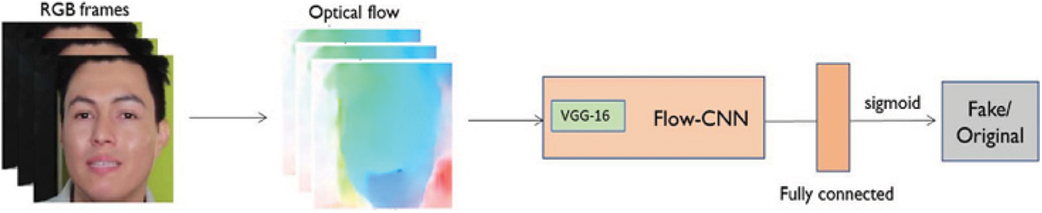
Figure 1: Basic structure of model

A fake detection approach is introduced based on the capsule network [10]. The pipeline of this model is shown in Fig. 2. The first step is image preprocessing. It depends on the input type, and a 300 × 300 input image size is used. Further, a part of pre-trained CNN is used along with several primary capsules for feature extraction. These features are then passed to a dynamic routing algorithm that calculates the agreement between these features. The result is forwarded to the corresponding output capsule.

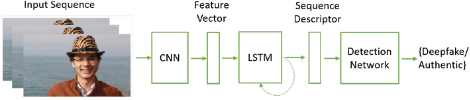
Figure 2: Capsule network-based fake detection model

Authors [11] proposed a benchmark for facial manipulation detection. This publicly available benchmark is created using the most common fake creation tools: Face Swap, Face2Face, Deepfake and Neural Texture. This benchmark is one of the largest databases as compared to its predecessors. They also used different state-of-the-art forgery detection techniques on their dataset, and their experiment shows that domain-specific knowledge helps to enhance the detector’s accuracy. The pipeline used is shown in Fig. 3.

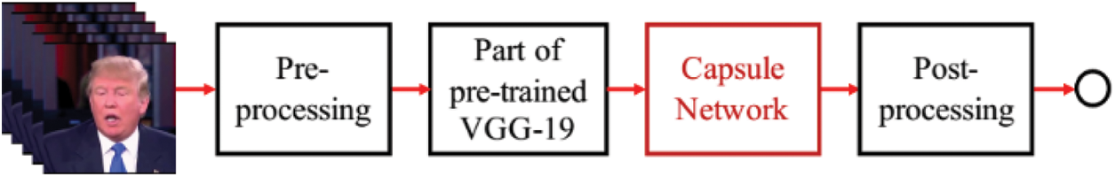
Figure 3: Pipeline used

Another approach in [12] discussed the temporal domain by incorporating Recurrent Neural Networks (RNN) on CNN. Fig. 4 shows the pipeline used in their method. Their convolutional Long short-term memory (LSTM) is based on two components; the first one is CNN for feature extraction, which is then passed to the second component LSTM for temporal features extraction which is then passed to the fully connected layer as sequence descriptor to compute the probability of video as fake or real. While the proposed method showed promising performance, this holistic approach had its drawbacks. It required both real and fake images as training data. It generated the fake images using the AI-based synthesis algorithm, which is less efficient than the simple mechanism for training data generation.

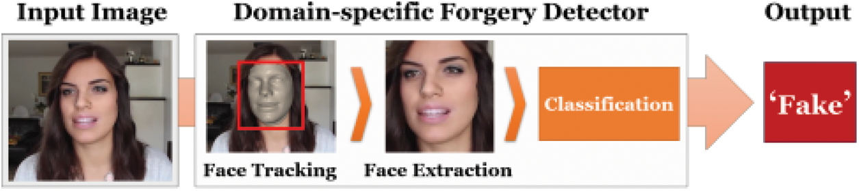
Figure 4: Pipeline

A novel learning-based deep fake detector was proposed by [13]. They presented a convolutional neural network based on an auto-encoder, which learns through a forensic embedding method and can transfer the network capability to new but similar manipulations. The encoder here encodes the image into a hidden space vector named h. This latent vector is subdivided as h0 and h1 for fake and real classes, respectively. During training, only the respective latent vector is activated for example, for fake classes, only h0 is activated, while during testing, both latent spaces are activated. The strength of activation determines the class of incoming images. The presented model can work on newly relevant manipulation techniques with only a small number of training examples and achieves good results on previously unseen examples.

A novel frequency analysis approach was presented in [14], based on the observation that deep fake and real images show a different spectrum at very high frequency. Thus, this property can be used to classify the real and fake images. Discrete signals are decomposed into sinusoidal components by using DFT (Discrete Fourier Transformation) method and azimuthal averaging is used to convert it into 1D signals. These signals are further converted into a feature vector by reducing the number of features without losing relevant information for using supervised (SVM and Logistic Regression) and unsupervised k-nearest neighbours (KNN) classifiers. The method shows promising results on FaceForensic++ and CelebA.

Another forgery localization and detection method was proposed in [15] called Manipulation Tracing Network for Detection and Localization (ManTra NET). It was an end-to-end solution to tempered localization region in an image. They treated the tempered region as an anomaly problem and used Long short-term memory (LSTM) to evaluate this local anomaly. Their method is tested on the Dresden image, copy move, splicing, and Kaggle camera model identification datasets with promising results.

Authors in [16] came up with a novel approach of signal analysis where they used spectrum as input instead of pixel input. They used this method based on their observation that in the common pipeline used by every generative adversarial network (GAN) algorithm to generate high-resolution fake images, the upper sampling layer leaves some artifacts in the frequency domain spectrum. These artifacts can be used to distinguish between real and fake images. They also used the simulation concept of GAN to match the common upper sampling method in All GAN methods. This helped the developers not to worry about access to the fake generation method. Experiments showed that the proposed method has achieved good performance on detecting images generated through GAN methods.

3  Proposed Methodology

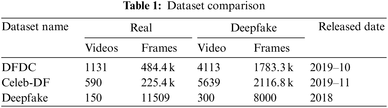
We used three different datasets by mixing them first and created a new dataset to train our ensemble model. The first one in the new mixed dataset contains an updated DFDC dataset, one of the largest datasets introduced in October 2019 and can be downloaded from the Kaggle repository1. It comprises approximately more than 5000 videos (real and manipulated). This dataset contains short video clips of actors and stars. In this dataset, manipulated videos are created using different face-swapping techniques. Dataset is enriched with various age groups of actors with different skin tones and gender. Gender distribution is 74% for females and 26% for males. Each video clip is approximately 15 s long and 4464 of the total videos are used as training sets and 780 of the total videos are used as a test set. We didn’t use the whole dataset because it is a huge dataset, which needs advanced resources and a large processing time. Currently, this is not possible for us due to limited resources. We selected 300 fake videos and 150 real videos from the whole dataset on a random basis to make it part of our new dataset.

The second dataset is another example of a large-scale dataset publicly available as Celeb-DF v2 (Celebrity DeepFake) released in November 2019 and can be downloaded from the GitHub repository2 by filling out a form to agree with copyright infringement rules. This dataset contains 6229 video clips with approximately 2342.2k frames of both manipulated and real videos. Each video in the dataset is approximately thirteen seconds long, containing 390 frames and 30 frames per second. Videos can be downloaded from YouTube containing 56.8% male subjects and 43.2% female subjects from different age groups. Swapping faces create fake videos; finally, the generated videos are stored in the MPEG 4.0 video file format.

The third dataset used to train our ensemble model is another publicly available dataset that can also be downloaded from the link given in a footnote3. Videos are manipulated using deep fake techniques. Following Table 1 shows the comparison of all three data sets used in our methodology:

Google Colab4 is one of the free machine learning tools provided by Google for educational and research purposes. It provides Tesla K80 GPU with approximately 12 GB of free RAM. A session of 12 h can be run in Colab interactive notebook after that the session expires automatically. This can be used in collaboration with Google drive in such a way that the Colab can be opened, and the drive can be mounted with it. In our working setup, the Colab notebook is set on Python and runtime is selected as GPU. The preprocessed dataset that we placed on Google drive is then mounted with Colab to import the data. With the installation of different software & libraries like Python 3, Tensorflow, Keras, OpenCV, Numpy, MatplotLib, Imutils, and OS we completed the working setup of our model.

From its development, CNN has gained huge popularity due to its flexibility and great performance in image preprocessing. CNN eliminates the need for manually extraction and one doesn’t need to select features required to classify the images because the CNN system can learn features. This feature extraction makes CNN’s well suited and accurate for most computer vision tasks. ConvNet (Convolutional Neural Network) are tremendously effective in image classification, speech recognition, and natural language processing.

CNN/ConvNet uses special convolution and pooling operations and performs parameter sharing. This enables ConvNets to run on any device, which makes them more attractive. We selected this CNN/ConvNet model for deep fake detection in our work. So, our next task was to determine which CNN-based model should be ensembled for our purpose. We found out that the network for deep fakes presented by [17] should be ensembled to fulfil our purpose, as we want to enhance the generalization ability in deep fake detection. It is a dense and lightweight network for face forensics. Our developed model of CNN is shown in Fig. 6 but to understand this model, first, we present Fig. 5 for the inception architecture used in our overall model in Fig. 6.

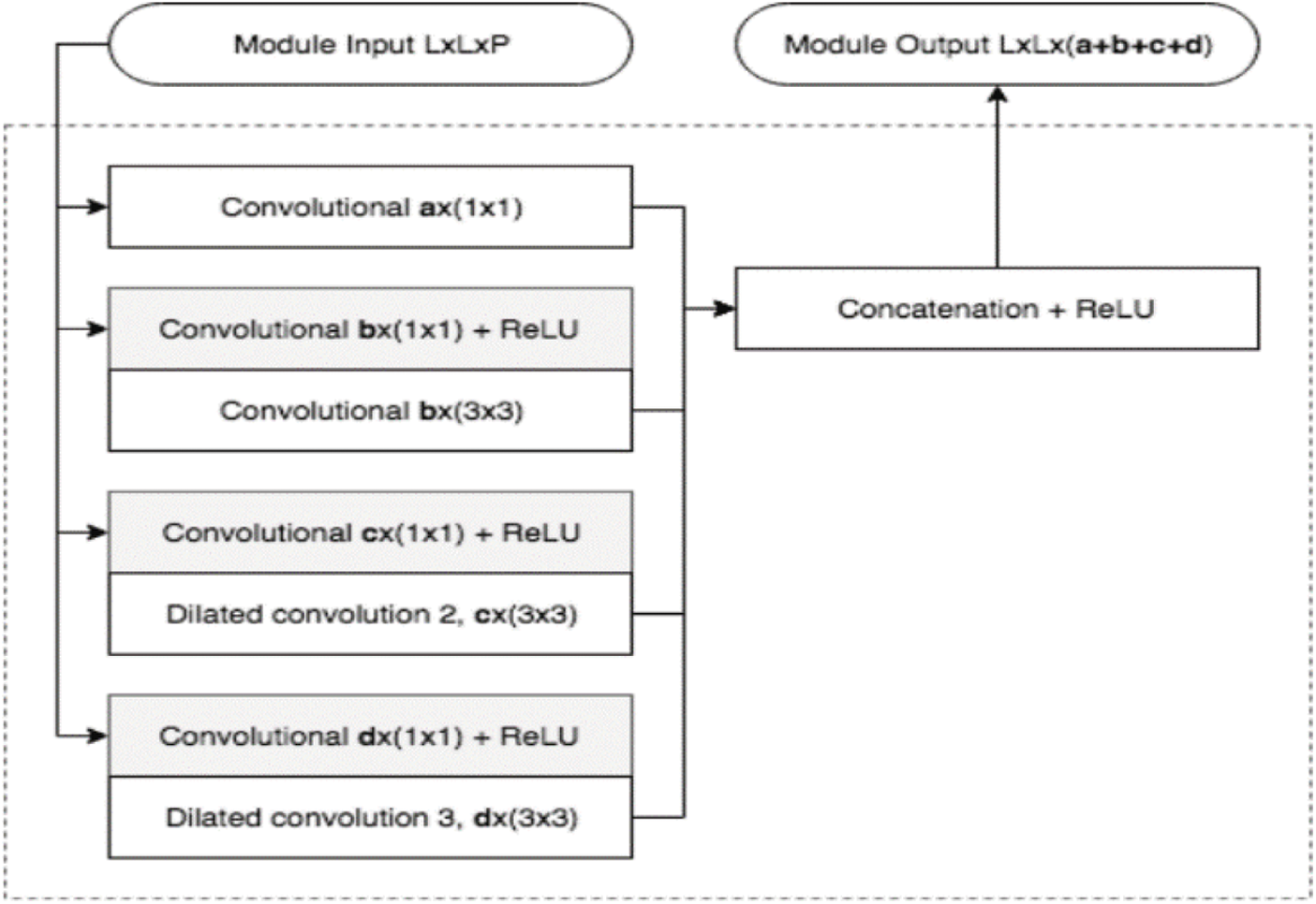
Figure 5: Inception architecture

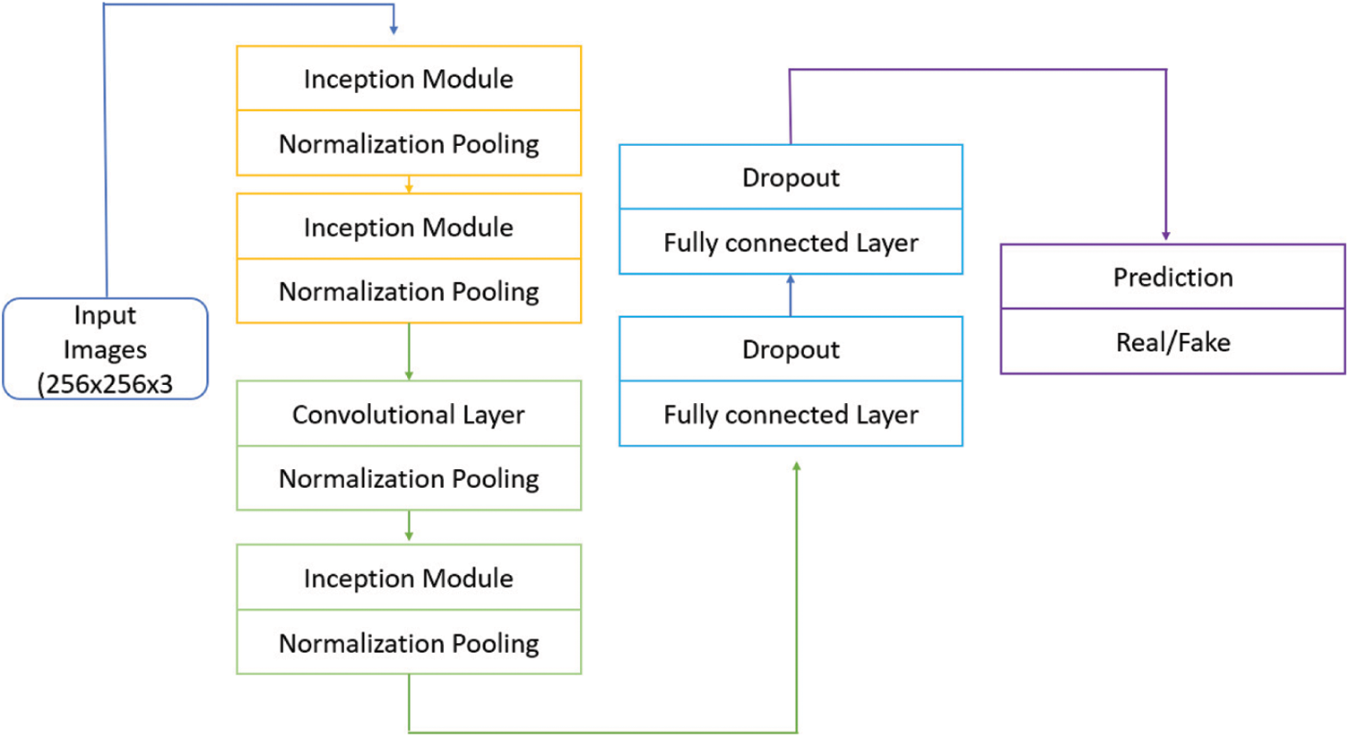
Figure 6: CNN model with inception module

The ensemble learning method is a way of improving the accuracy and performance of the model using a group of classifiers to solve the same problem and then combining their output using one of the combining methods available to generate ensemble output. we ensembled three CNN-based classifiers in our work discussed next, hence calling it ECNN. Literature shows that ensemble always helps in most cases and can produce good results compared to a single classifier. There are different ensemble methods available. This is where we have put our effort into finalizing those optimal methods. We are utilizing the power of the ensemble bagging method, which is described with its basic algorithm next in Fig. 7.

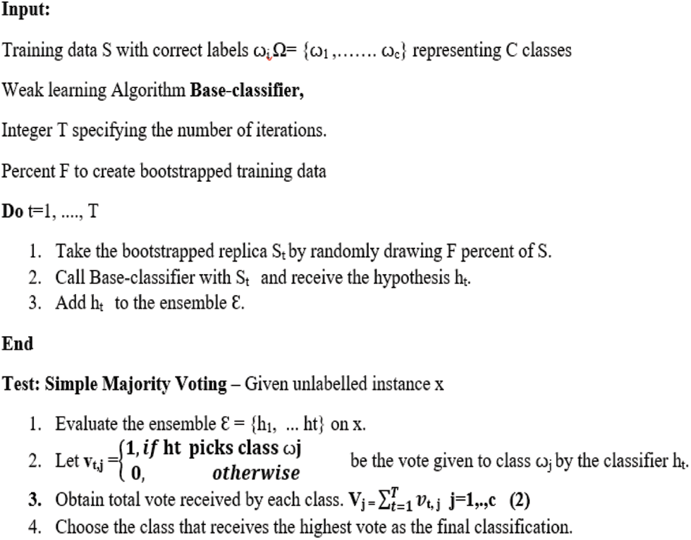
Figure 7: Bagging algorithm elaborate ensemble model

Bootstrap aggregation or bagging is one of the simplest ensemble-based methods with good performance. The classifier diversity is obtained in bootstrap aggregation by randomly drawing the training dataset from the whole dataset. A different subset of data is drawn randomly from the whole set of data in a way that no, or few data samples, or repeated in each subset, are used to train different classifiers of the same kind. Then finally, the output from each classifier is combined using the max voting method in which ensemble output is the decision of majority classifiers, as displayed in Fig. 6. Further, the basic algorithm for bootstrap aggregation is shown in Fig. 7.

In the figure mentioned above, we can see that we need a training dataset with its correct labels and base classifiers to train T a number of times. Percent F is the fraction of the dataset for each classifier drawn randomly from the whole dataset. Then each classifier is trained, and its results are stored as discussed next.

While testing, unlabeled instances are given to the ensemble hypothesis, and each base-classifier present in this ensemble will generate a result for this instance after receiving the total votes from each base classifier. Max voting or majority voting assigns the class to this unlabeled instance.

On testing an image, two classifiers classify it into fake class, and one classifies it as real, then ensemble output by majority vote from all classifiers is fake in this example, which means ensemble output is the class assigned by the most classifiers. The basic workflow of the ensemble convolutional neural network (ECNN) model can be viewed in Fig. 8, and each step in the workflow is detailed as follows.

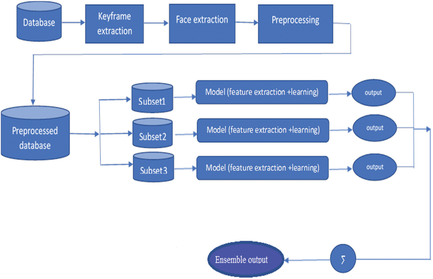
Figure 8: Workflow of the ECNN ensemble model

In Fig. 8, the dataset consists of videos of celebrities with their correct labels and is passed through a process of conversion into suitable input according to the model requirement presented as follows. The first three steps in the figure are performed offline. Our ECNN model works with images, so we need to convert the incoming videos into frames/images. Each video in our dataset consists of approximately 300 frames; we extracted these with a speed of 30 frames per second from each video. These frames are then stored in jpeg format in two different folders. The first folder is named as ‘fake’ and contains frames from fake videos; the other folder is named’ real’, which contains frames from the real videos. These frames then become the input of the next step as follows.

As deep fakes are most used to change the identity or expression of the person, and work is performed mostly on the facial region, which also leaves inconsistencies in facial structures, compression rate and other dissimilarities in the manipulated region. Our proposed ECNN model can detect these inconsistencies, which is then used to differentiate between fake and real videos. In this phase, only the manipulated region extracted from the image is the face in our case. We used Voila John’s facial extraction model5, one of the best models among the others available for face detection. The output of this step becomes the input of the step discussed next. Extracted faces from the previous step are then passed to preprocessing phase, which is done offline on the system. Each image is rescaled to 128 × 128 pixels. Other operations like brightness, zooming, etc., are done and generated data is stored in a preprocessed directory. Once the mentioned steps are over for each subset of the dataset, the preprocessed dataset is then uploaded on Google drive, which is then mounted with Colab to import the data into the active notebook environment.

After the preprocessing, subject datasets are passed to each classifier of the same architecture discussed in Fig. 6. The first two layers receive output from inception modules and the other two are simple convolutional layers with 16 filters with filter size 5 × 5 and Relu activation function is applied. Then batch normalization and the max-pooling layer are added with pool size 2 × 2 to reduce the dimensions. After that flattening layer is used to obtain a linear vector with full connections. Then two dense layers are applied: the first uses Relu activation function and the second uses the sigmoid activation function. The image is passed through all ECNN layers and here, the classification is done, and the model finally predicts the class of test images. The output of each classifier in Fig. 8 is a video on which a bounding box appeared on a person’s face with its label as fake or real. Ensemble output is the output picked up by the Bagging algorithm Fig. 7 in the ensemble model. As we have three classifiers/models, the output selected by at least two models would be declared as ensemble output. We have two different settings for our ensemble approach.

Three classifiers of the model presented are created as shown in Fig. 8 and each classifier is trained on a dataset which is a combination of all these databases including DFCD, Celeb DF v2, and deep fake. We drew 300 fake and 150 real videos from each dataset respectively and combined them to create the training dataset for our ensemble model. Then three subsets of data are randomly drawn from the newly made training dataset to train each classifier in the ensemble model. It is pertinent to note that we have used the same workflow depicted in Fig. 8.

Evaluation is a method of measuring the performance of a model. It aims to measure the accuracy of a model on previously unseen data. There are two different ways to evaluate a model performance: holdout and cross-validation. Both methods used a set of unseen data to evaluate model performance. The use of unseen data to evaluate the model is a way to avoid overfitting. We used the holdout method to evaluate the model in which the dataset is divided into three sets of training, validation, and testing.

Secondly, we used the evaluation metrics to measure the model’s performance. Different metrics can be used to evaluate the model, but we have used the confusion matrix to evaluate our model. The confusion matrix plots the detailed information about four outcomes i.e., true positive, false positive, true negative and false negative.

With the help of the confusion matrix, we can compute the following important information about the performance of our model.

True Positive Rate (TPR)= TP /(TP+FN)(1)

False Positive Rate (FPR)=1−Specificity=1−(TN /(TN+FP))(2)

The accuracy of a model is way of expressing how frequently a classifier classifies an object correctly it can be calculated using the following equation

Accuracy =(TP+TN)/(TP+TN+FP+FN)(3)

Error Rate can be defined as the inaccurate prediction of a classifier among all data is termed an error rate or EER and can be computed using the following equation.

Error Rate =1− accuracy=(FP+FN)/(TP+TN+FP+FN)(4)

Precision is defined as the portion of related instances among all repossessed instances. Mathematically it can be computed as below.

Precision =TP/(TP+FP)(5)

F-measure is a commonly used method to evaluate binary classifiers. It is a way of determining the test accuracy of a model and can be calculated using the following equation.

F−measure:2/((1/Precision)+(1/Recall))(6)

On our dataset discussed earlier in Table 1, the model is evaluated using Eqs. (1) to (6) and the results are detailed in the results section.

4  Results & Discussion

Different parameter values are used in our ECNN model to get better results. Using these parameters, we observed that the ECNN model achieved good accuracy on the provided dataset as compared to existing methods. The soft Max layer in ECNN is used as an optimizer with a learning rate of 0.001. The batch size is set to 16, which is limited due to GPU memory. The total number of epochs used is 20, with sample per epoch is 1000. The results and performance of the model are discussed as follows.

After selecting the dataset, the training dataset is divided into three subsets, which are used to train each base classifier in the ensemble model. A separate holdout dataset is kept from deep fake detection database, which is checked on the model during the development. Training and testing accuracy and model loss can be seen in Figs. 9 and 10, respectively. This shows that the accuracy only approaches 100% at epochs 5 and 17. At epoch 13 and afterwards, the training and testing accuracy remain the same but a little below to 100%.

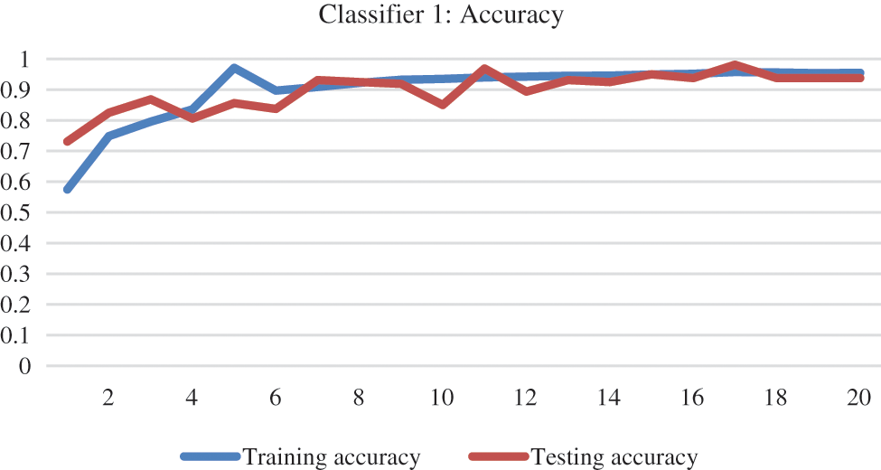
Figure 9: Training and testing accuracy base classifier 1

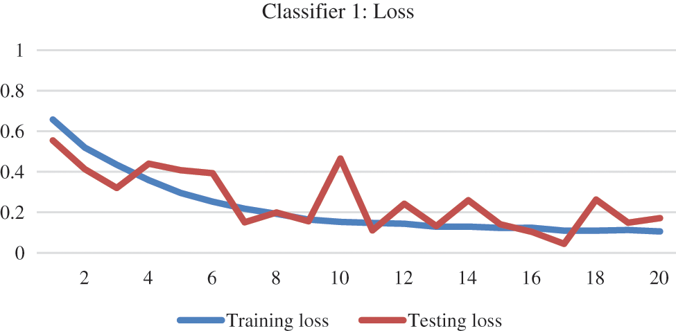
Figure 10: Training and testing loss base classifier 1

The loss of classifier 1 was higher initially, which was more than 50% and then gradually decreased to almost 20% at the end, as can be seen in Fig. 10. Trends in training and testing accuracy along with the model loss for base classifier 2 can be viewed in Figs. 11 and 12.

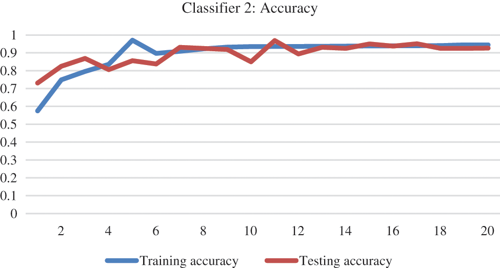
Figure 11: Accuracy of base classifier 2

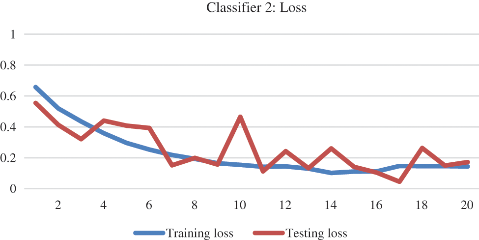
Figure 12: Training and testing loss for base classifier 2

Base classifier 3 of the ECNN model is trained and tested on its respective dataset. The results are depicted in the graphical representation of accuracy and loss function in Figs. 13 and 14.

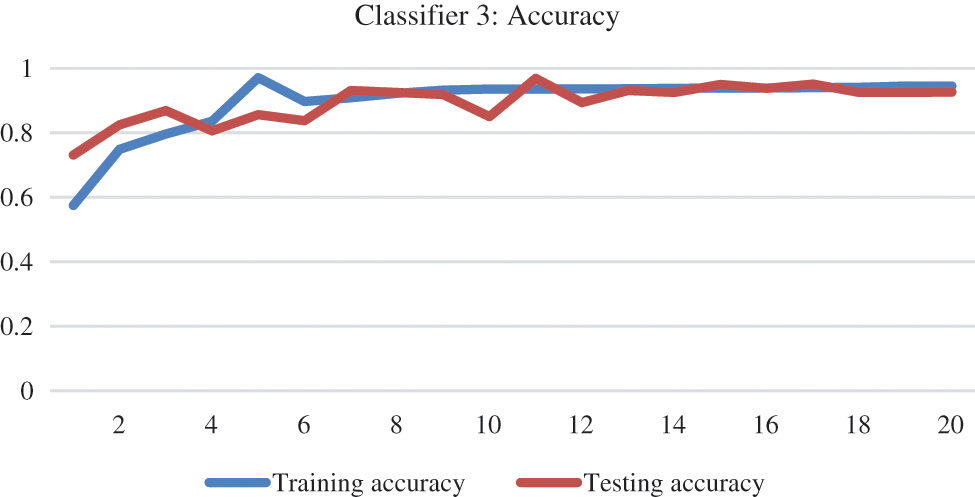
Figure 13: Accuracy of base classifier 3

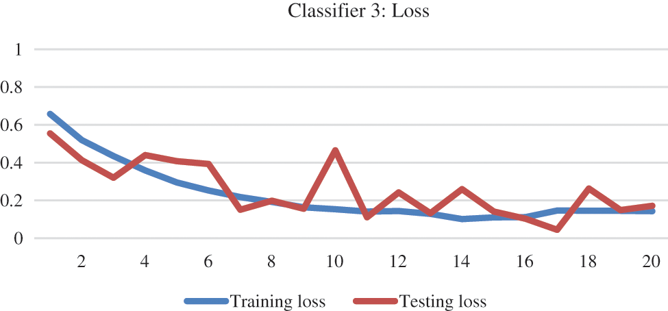
Figure 14: Training and testing loss of base classifier 3

Similarly, the confusion matrix drawn can be seen in Fig. 15. This shows the performance of the ensemble model using these values. With the help of this matrix, we calculated the following results of our ensemble model.

TPR=TP/(TP+FN)=80/(80+3)=0.9639FPR =1−(TN/(TN+FP))=1−(6/(6+97))=0.32Accuracy =(TP+TN)/(TP+TN+FP+FN)=(80+16)/(80+16+3+1)=0.96

EER=1-- accuracy =1−0.96=0.04Precision=TP/(TP+FP)=80/(80+1)=0.9876Recall =TP/(TP+FN)=80/(80+3)=0.9639F−measure =2/((1/Precision)+(1/Recall))=2/((1/0.9876)+(1/0.9639))=2/(1.0125+1.0374)=0.9697

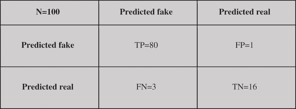
Figure 15: Confusion matrix for the CNN ensemble model

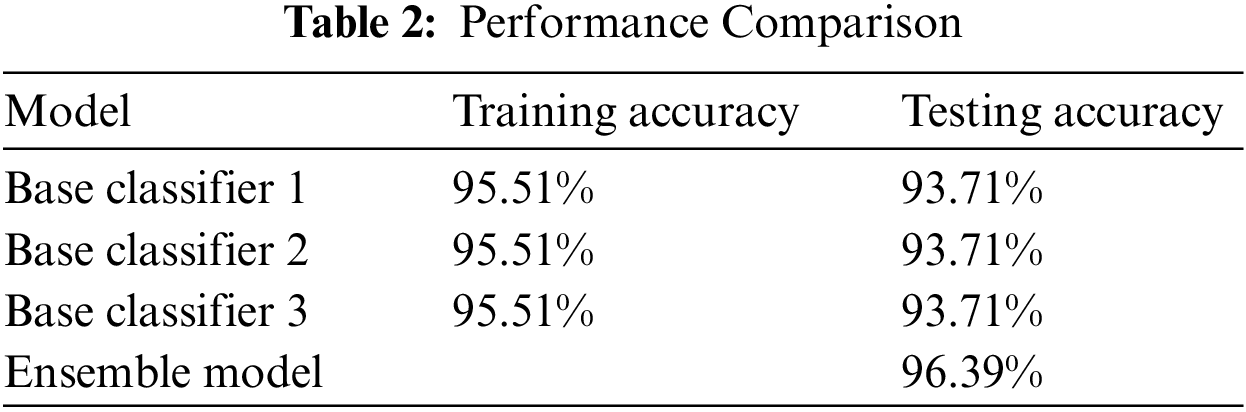
From Table 2, we can see that classifier 1 reaches 95.51% and 93.17% training and testing accuracy, respectively. Overall, the ensemble classifier performs 96% on the testing dataset, which is better than the single classifier. The detailed comparison of performances of all classifiers on deep fake detection datasets can be seen in Table 2.

A video is passed to the model as input. This video is converted into frames and the face extraction algorithm extracts the faces from these frames then, these faces are passed to all three base classifiers and each classifier predicts the face into one of the two classes and the final output is computed by taking the maximum output from the base classifiers. A video is classified as fake if at least 50 frames from that video are classified as fake. In Fig. 16, all three base classifiers classify the incoming frame as real thus the final output known as ensemble output is also real. A few examples are shown below to see how each video frame’s final prediction is computed.

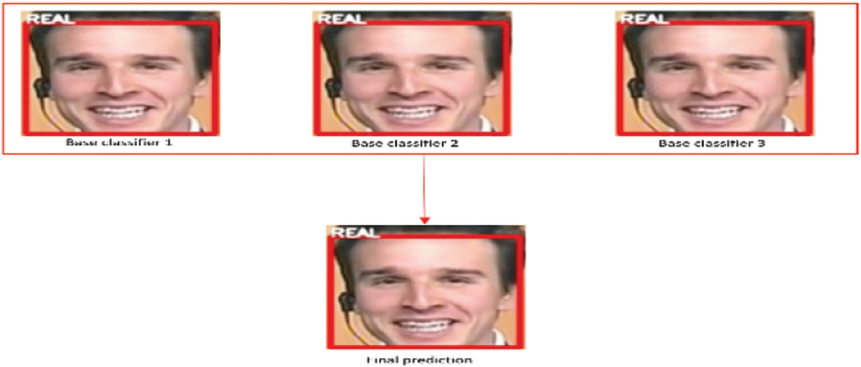
Figure 16: Ensemble output 1

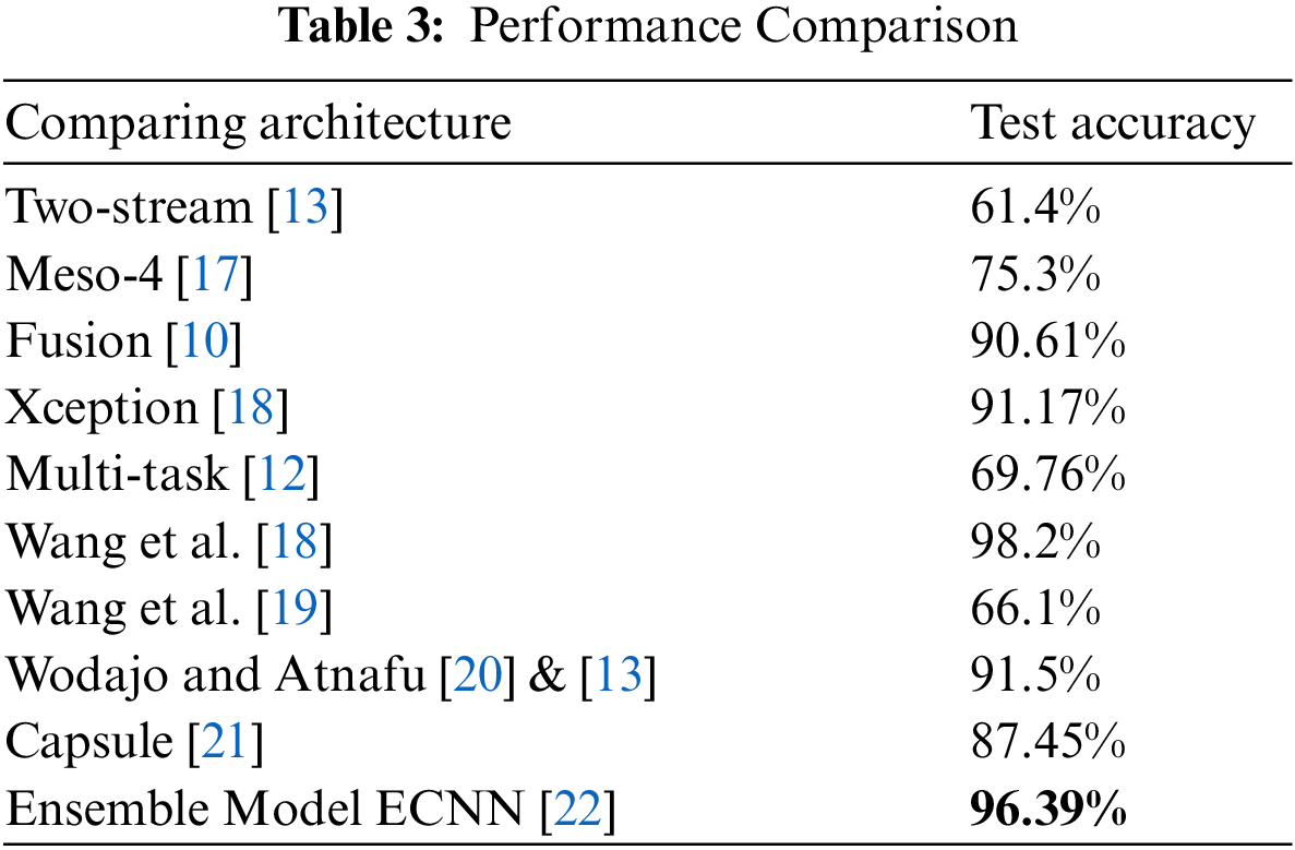
In Fig. 17, two base classifiers classify the image as real, whereas one classifies it as fake. Ensemble output is the maximum number of the same outputs from these base classifiers, so in this case ensemble model classifies the image into real. We compared the performance of our ensemble model with other state-of-the-art models on deep fake detection challenging dataset. This includes Two-stream, Meso-4, Fusion, etc. The comparison showed that the proposed method of ECNN has outperformed the other state-of-the-art methods except for the fusion-based technique (which contains features of eyes, nose, mouth, etc.) discussed by Wang et al. [18], which is also a CNN-based technique. Still, more focus is put on preparing datasets with special fusion-related features.

Figure 17: Ensemble output 2

Table 3 have shown that deep learning-based models can perform better than the other approaches. Besides our work in the table, the deep learning model with state-of-the-art results on the DFDC dataset is also available.

5  Conclusion

Deep learning helps people generate more realistic fake material which the naked eye cannot detect. To detect these forged media, we need some deep learning methods that might help us detect them and can be helpful for victims. Deepfake technology is potentially used in entertainment, education, e-commerce and in many other industries. It also helps in saving a lot of time, effort, and money, but this technology’s drawbacks cannot be avoided and require some serious attention. It can enhance performance and generalization. Our ensemble model ECNN attempts to make fake video detection much better. Ensemble methods are techniques that create multiple models and combine them to produce improved results. Ensemble methods usually produce more accurate solutions than a single model would. In several machine learning competitions, where the winning solutions used ensemble methods. There are different ensemble techniques, but we used the ensemble bagging method due its simplicity.

Acknowledgement: Thank you to our coworkers for their moral and technical assistance.

Funding Statement: This research is supported by the Deanship of Scientific Research, Islamic University of Madinah, KSA.

Conflicts of Interest: The authors declare that they have no conflicts of interest to report regarding the present study.

1https://www.kaggle.com/c/deepfake-detection-challenge/data.

2https://github.com/yuezunli/celeb-deepfakeforensics.

3https://my.pcloud.com/publink/show?code=XZLGvd7ZI9LjgIy7iOLzXBG5RNJzGFQzhTRy.

4https://colab.research.google.com/notebooks/intro.ipynb.

5https://www.mygreatlearning.com/blog/viola-jones-algorithm/.

References

1. L. Xie, W. Zhong, W. Shi and S. Sun, “Spectrum of fungal keratitis in North China,” Ophthalmology, vol. 113, pp. 1943–1948, 2006. [Google Scholar]
2. M. Li and L. Zhang, “Research advance of fungal keratitis,” International Journal of Ophthalmology and Clinical Research, vol. 8, no. 2, pp. 384–387, 2008. [Google Scholar]
3. S. Belliappa, J. Hade, S. Kim, B. D. Ayres and D. S. Chu, “Surgical outcomes in cases of contact lens-related fusarium keratitis,” Eye Contact Lens, vol. 36, pp. 190–194, 2010. [Google Scholar]
4. L. Xie, H. Zhai, J. Zhao, S. Sun and X. Dong, “Antifungal susceptibility for common pathogens of fungal keratitis in shandong province, China,” American Journal of Ophthalmology, vol. 146, no. 2, pp. 260–265, 2008. [Google Scholar]
5. M. A. Dahlgren, A. Lingappan and K. R. Wilhelmus, “The clinical diagnosis of microbial keratitis,” American Journal of Ophthalmology, vol. 143, no. 6, pp. 940–944, 2007. [Google Scholar]
6. P. Kryszkiewicz, A. Kliks and H. Bogucka, “Small-scale spectrum aggregation and sharing,” IEEE Journal Selected Areas Communication, vol. 34, no. 10, pp. 2630–2641, 2016. [Google Scholar]
7. Q. Qiu, Z. Liu, Y. Zhao, D. Wei and X. Wu, “Automatic detecting cornea fungi based on texture analysis,” in IEEE Int. Conf. on Smart Cloud, China, no. 5, 2016. [Google Scholar]
8. F. Riaz, A. Hassan, S. Rehman and U. Qamar, “Texture classication using rotation and scale invariant gabor texture features,” IEEE Signal Process Letter, vol. 20, no. 6, pp. 607–610, 2013. [Google Scholar]
9. L. S. Davis, S. A. Johns and J. K. Aggarwal, “Texture analysis using generalized co-occurrence matrices,” IEEE Transactions on Pattern Analysis and Machine Intelligence, vol. 1, no. 3, pp. 251–259, 1979. [Google Scholar]
10. D. A. Clausi and H. Deng, “Design-based texture feature fusion using gaborlters and co-occurrence probabilities,” IEEE Transactions on Image Processing, vol. 14, no. 7, pp. 925–936, 2005. [Google Scholar]
11. T. Ojala, K. Valkealahti, E. Oja and M. Pietikäinen, “Texture discrimination with multidimensional distributions of signed gray-level differences,” Pattern Recognition, vol. 34, no. 3, pp. 727–739, 2001. [Google Scholar]
12. Z. Li, S. Guo, L. Yu and V. Chang, “Evidence-efficient affinity propagation scheme for virtual machine placement in data center,” IEEE Access, vol. 8, pp. 158356–158368, 2020. [Google Scholar]
13. N. Naz, S. Abbas, M. Adnan and M. Farrukh, “Efficient load balancing in cloud computing using multi-layered mamdani fuzzy inference expert system,” International Journal of Advanced Computer Science and Applications (IJACSA), vol. 10, no. 3, pp. 569–577, 2019. [Google Scholar]
14. R. Rahim, “Comparative analysis of membership function on Mamdani fuzzy inference system for decision making,” Journal of Physics, vol. 930, no. 1, pp. 012029, 2017. [Google Scholar]
15. N. Iqbal, S. Abbas, M. A. Khan, T. Alyas, A. Fatima et al., “An RGB image cipher using chaotic systems, 15-puzzle problem and DNA computing,” IEEE Access, vol. 7, pp. 174051–174071, 2019. [Google Scholar]
16. T. Alyas, I. Javed, A. Namoun, A. Tufail, S. Alshmrany et al., “Live migration of virtual machines using a mamdani fuzzy inference system,” Computers, Materials & Continua, vol. 71, no. 2, pp. 3019–3033, 2022. [Google Scholar]
17. D. Zhang, J. Hu, F. Li, X. Ding, A. K. Sangaiah et al., “Small object detection via precise region-based fully convolutional networks,” Computers, Materials and Continua, vol. 69, no. 2, pp. 1503–1517, 2021. [Google Scholar]
18. J. Wang, Y. Wu, S. He, P. K. Sharma, X. Yu et al., “Lightweight single image super-resolution convolution neural network in portable device,” KSII Transactions on Internet and Information Systems, vol. 15, no. 11, pp. 4065–4083, 2021. [Google Scholar]
19. J. Wang, Y. Zou, P. Lei, R. S. Sherratt and L. Wang, “Research on recurrent neural network based crack opening prediction of concrete dam,” Journal of Internet Technology, vol. 21, no. 4, pp. 1161–1169, 2020. [Google Scholar]
20. S. He, Z. Li, Y. Tang, Z. Liao, F. Li et al., “Parameters compressing in deep learning,” Computers Materials & Continua, vol. 62, no. 1, pp. 321–336, 2020. [Google Scholar]
21. A. Alzahrani, T. Alyas, K. Alissa, Q. Abbas, Y. Alsaawy et al., “Hybrid approach for improving the performance of data reliability,” Sensors, vol. 22, no. 16, pp. 1–19, 2022. [Google Scholar]
22. B. Zafar, S. A. Z. Naqvi, M. Ahsan, A. Ditta, U. Baneen et al., “Enhancing collaborative and geometric multi-kernel learning using deep neural network,” Computers, Materials & Continua, vol. 72, no. 3, pp. 5099–5116, 2022. [Google Scholar]
Cite This Article
Copyright © 2023 The Author(s). Published by Tech Science Press.
This work is licensed under a Creative Commons Attribution 4.0 International License , which permits unrestricted use, distribution, and reproduction in any medium, provided the original work is properly cited.
Downloads
Citation Tools