Improved Symbiotic Organism Search with Deep Learning for Industrial Fault Diagnosis

1  Introduction

In industrial production, any faults of rotating machines might lead to massive economic losses. Hence, fault diagnosis (FD) and fault detection become vital to the operative safety of latest production system [1]. Owing to the lack of fault samples, complications of fault kinds, problems of FD, and higher cost of manual annotation samples, the under small samples are still a research domain which requires continuous update, continual progress, and optimization [2,3]. With the continual growth of modern manufacturing sector, rotating machinery plays a crucial role in complicated electromechanical equipment, can be advanced toward complexity, intelligence, and large scale [4,5]. Rotating machinery generally operates for longer duration under high speeds and heavy loads. Bearing, gearboxes, and other significant elements were probably to suffer from fracture, wear, deformation, and other faults at the time under time-varying operating conditions and inherent degradation process [6]. The failure of such elements would affect the normal function and equipment usage [7].

Serious cases could lead to damage or downtime and they might occur huge economic losses and casualties [8,9]. Thus, research relating to condition monitoring and FD of rotating machinery was one such key which assures the normal function of equipment, minimizes unplanned maintenance, ignored catastrophic failures, and assures the security of industrial production that was most important one [10]. Main tasks of FD research on rotating machinery involve determination of functioning state, determining the fault kind, and estimating the fault trend. Recently, authors have made many research studies in the domain of rotating machinery FD that reached productive research outcomes and were implied in actual working states [11,12]. With the speedy advancement of intellectual methods, the recent study on deep learning (DL) in the FD of rotating machinery was rising year by year, and it grabbed the interest of many authors. For the promotion of the research growth in this domain, the paper assesses the related research from the two prospects of DL concept and its applications in FD [13]. (Research could grant inspiration and convenience for related authors and offer references for promoting and understanding the advancement of FD research.

This article presents an improved symbiotic organism search with deep learning enabled fault diagnosis (ISOSDL-FD) model for gearbox fault detection in industrial systems. The proposed ISOSDL-FD technique applies a Fast kurtogram based time-frequency analysis for revealing the energy present in the machinery signals in the time and frequency representation. In addition, the deep bidirectional recurrent neural network (DBiRNN) is applied for fault detection and classification. At last, the ISOS method can be derived for optimal hyperparameter tuning of the DL approach. To illustrate the improvised performance of the ISOSDL-FD algorithm, a comprehensive experimental analysis was performed.

The rest of the paper is organized as follows. Section 2 offers the literature review, Section 3 elaborates the proposed ISOSDL-FD model, Section 4 provides performance validation, and Section 5 concludes the paper.

2  Literature Review

Wang et al. [14] suggest a novel fault prognosis technique has infrared thermal images and least-square-interactive-support-matrix-machine (LSISMM). In this technique, a new matrix-form classifier known as LSISMM can be created over the idea of non-parallel interactive hyperplane to completely use the structure data of infrared thermal imageries. To enhance the computational efficacy, innovative least square loss constraints were projected for LSISMM. Additionally, the researchers extract an effectual solution structure on the basis of the alternative direction technique of the multiplier (ADMM) structure. In [15], an adaptive convolutional neural network (CNN) was built on the basis of the ontology representation of pump. Firstly, time–frequency features of pressure signals were acquired through continual wavelet transformation. Secondly, establishment of a deep CNN by setting initial hyperparameter. Thirdly, Bayesian optimization can be leveraged for achieving automatic learning of main significant hyperparameters for constructing an adaptive CNN. In [16], a new FD technique for rotating machinery on the basis of deep residual neural network (DRNN) and data fusion was suggested. Initially, the frequency domain and time domain features of the original signal were derived via the Short-time Fourier transform (STFT) layer, after which the DRNN and the fusion embedding layers were utilized for fusing the frequency domain, spatial domain, and time domain features for obtaining high quality low-dimension fusion features.

An FD technique for rotating machinery in time varying circumstances on the basis of DL and tacholess order tracking (TOT) was suggested in [14]. At first, estimated speed information and frequency domain periodic signals were attained by tracking the order. Next, the frequency domain periodic signals refer to a speed which can be standardized with the help of estimated speed data. At last, standardized features were derived by DL method for making feature vectors. The feature vector can be fed to softmax layers to finish FD of the gearboxes. Li et al. [17] advance an FD technique with the help of CNN for InfRared Thermal (IRT) images. Firstly, IRT method can be used for capturing the IRT images of rotating machinery. Secondly, the CNN can be implied for extraction of fault features from the IRT images. Finally, the acquired features were fed to the Softmax Regression (SR) classification for fault pattern identification. In [18], a novel DL related FD technique, that derives features from frequency as well as time domains were suggested. A set of 2 deep features from several domain was merged into global principle component analysis and intrinsic low-dimensional features by local. And a novel ensemble kernel extreme learning machine was suggested for fault pattern classifier on the basis of the fused feature.

3  The Proposed Model

In this study, a new ISOSDL-FD technique was introduced for the recognition of faults in industrial systems. The proposed ISOSDL-FD technique accomplished proficient identification and classification of faults in the gearbox data. In addition, a Fast kurtogram based time-frequency analysis is used for revealing the energy present in the machinery signals in the time and frequency representation. Moreover, the ISOS-DBiRNN is applied for fault detection and classification. Fig. 1 depicts the overall process of ISOSDL-FD approach.

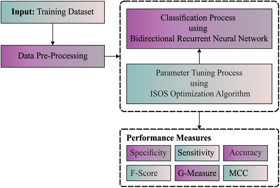
Figure 1: Overall process of ISOSDL-FD approach

3.1 Time Frequency Analysis

Time-frequency analysis was helpful for revealing the energy restricted from the machinery signal from the time and frequency representation [19]. Different kinds of time-frequency transformations like spectral kurtosis diagram (kurtogram), wavelet transform (WT), empirical mode decomposition (EMD), and STFT are utilized to machinery FD. But, every approach are flaws. It can be complex for selecting the mother wavelet function to WT, but EMD models offer in mode mixing problems. Besides, in STFT approaches, the time and frequency resolutions were connected together. The fast kurtogram system offers any benefits on other methodologies as the present generation of fast kurtogram doesn’t need some parameters that set, creating the model simple for utilizing. So, the fast kurtogram has been selected to the presented analysis model for reducing the amount of parameters which required that set. The kurtogram is 4th order of spectral diagnosis that is called spectral kurtosis. Antoni imposed 4 constraints on kurtogram diagnosis for increasing the versatility of procedure that creates the method further sensitive to non-stationary signals. The kurtogram is determined utilizing in Eq. (1):

kxf(x)=⟨H4(t,f)⟩⟨H2(t,f)⟩2−2,(1)

whereas ⟨.⟩ implies the operator of time averaging and H(t,f) denotes the enveloped procedure of signals x(t). H(t,f)has been evaluated utilizing in Eq. (2):

H(t,f)=Σn=tt+Nn−1w(n−t)x(n)e−j2πfn(2)

In which w(t) represents the length of windows.

3.2 Fault Detection and Classification Model

In this study, the DBiRNN is applied for fault detection and classification. The prediction network is carried out by means of a Recurrent Neural Network (RNN) [20]. The neural network takes the temporal series of observation Xt=(xt−T−1,xt−T−2,…,xt) as input, and generate a series of vectors (ht−T−1xt−T−2,…,ht) through a nonlinear activation. The output vector is hidden variable that describes the distribution of observation. Unlike the conventional feedforward neural network, an RNN considers previous data or named “memory”. The label is defined using a nonlinear mapping over this hidden variable and it is mathematically expressed in the subsequent formula.

ht=H(Wxhxt+Whhht−1+bh)(3)

Yt=F(Whyht+by)(4)

Now, H refers to a nonlinear function that is selected from sigmoid and tanh. Fis generally selected from softmax or sigmoid when the output label is independent or mutually exclusive correspondingly. Wand b are related weight (for example Wxh represent the input-hidden weight matrixes), and bias (for example, bh is hidden bias vector) matrix correspondingly. The parameter is learned from the trained dataset. In recent times, researcher demonstrates a problem using simple RNN structure where the gradient disappears. In order to resolve the issue, the most common replacement is Gated Recurrent Unit (GRU) cells and Long Short-Term Memory (LSTM) that maintains their state over time, which leads to captured long term dependency within time sequence data. In this study, the version of GRU cell and LSTM utilized are correspondingly.

h!=HLSTM(xtht−1,ct−1)(5)

ht=HGRU(xtht−1)(6)

The main distinction among GRU and LSTM is that the content of GRU cell memory is exposed continuously to output and it is easily implemented because it needs fewer parameters in the network. Briefly, the RNN cell HX(.) can be LSTM (Eq. (5)) or GRU cell (Eq. (6)) RNN. One drawback of RNN is that they can utilize preceding context. But with a windowed approach where entire temporal context is available, there is no reason not to utilize future context. The Bi-directional RNN (BiRNN) with elementary RNN unit achieves this aim by data processing in these two directions with two discrete hidden layers that are later fed to the output layer in similar fashion. A BiRNN calculates the output sequenceyt, h→t forward hidden sequence, and h←t the backward hidden sequence the by reiterating the forward layer from t to t−T+1, the backward layer from t−T+1 to t, and later update the output layer:

h→=H(Wxh→xt+Wh→h→h→t−1+bh→)(7)

h←t=H(Wxh→xt+Wh←h←h←t−1+bh←)(8)

yt=F(Wh→yh→+Wh←yh←t+by)(9)

Assisting LSTM with this bi-directional learning ability allows the system to access long-range context in input direction and enrich sequence data understanding. With the potential to disentangle complicated temporal dependency, deep RNN is constructed by stacking various RNN hidden layers, with the output series of one layer form the input series for the following. Assume the same hidden layer as for each N layer in the stack, the hidden vector sequence hn is computed iteratively from n=1 to N and t−T+1 to t:

h!=H(Whn−1hnh+n−1+Whnhnht−1n+bhn)(10)

yt=F(WhNyhtN+by)(11)

where h0=x.

DBiRNN is implemented by replacing every hm hidden sequence with hm→ and hm← the backward and forward sequences, and ensures that each hidden layer receives input from the backward and forward layers. Deep architecture is attained by replacing every RNN unit in the DBiRNN by a deep uni-directional RNN. Fig. 2 showcases the infrastructure of Bi-directional RNN. Therefore, for M stacked BiRNN and every backward and forward cell have N stacked RNN structure, we attain a 2×M×N RNN unit system. But we found that deep configuration doesn’t produce improved performance on limited data as they overfit the training dataset. Hence, we use single Bi-LSTM stacked with single uni-directional GRU cell yields a three RNN unit system, as

(h→t1,c→t1)=HLSTM(xt,h→t−11,c→t−11)(12)

(h←t1,c←t1)=HLSTM(xt,h←t−11,c←t−11)(13)

ht2=HGRU([h→t1:h←t1],ht−12)(14)

Yt=F(Wh2yht2+by)(15)

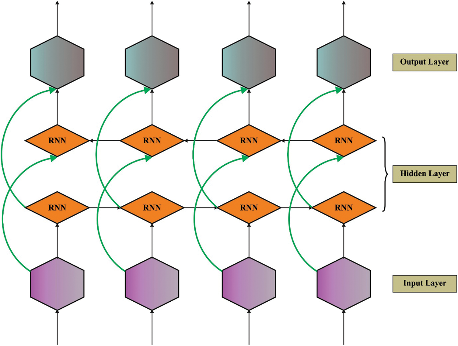
Figure 2: Structure of Bi-directional RNN

3.3 Hyperparameter Tuning Model

At the final stage, the ISOS algorithm is derived for optimal hyperparameter tuning of the DL model in such a way that the classification performance gets improved. The SOS algorithm was first introduced by Cheng et al. [21]. The SOS technique is the new methodology to solve optimization problems depends on organism interaction in nature. Organism rarely lives in isolation because of the dependence on other species for survival and nutrition. This relation depends on trust that is called a symbiotic relationship. The process initiates by a population initialization named the ecosystem. During the primary ecosystem, a group of organisms is randomly generated. Every organism represents a proposed solution for the problem. The time complexity in the SOS is characterized as n2. The SOS renders a new solution according to the biological relations among the two living organisms. It consists of Mutualism, Commensalism, and Parasitism of biological relationships.

3.3.1 Mutualism

Currently, both organism benefits from the relationships they have with one another. Assume honeybee relationships with flowers, for instance, the bees fly over the flower for collecting the nectar needed to produce honey. Also, it is useful to the flower since bees, scattering the pollen, facilitate their pollination. In this study, Xi refers to an organism equivalent to i−th individuals in nature. Then, Xj is selected at a random fashion and related to the Xi in nature. At last, Xi and Xj upgraded based on the following equation:

Xinew=Xi+rand(0,1)×(Xbest−Mutua1−Vector×BF1)(16)

Xjnew=Xj+rand(0,1)×(Xbest−Mutua1−Vector×BF2)(17)

MutualVector=Xi+Xj2(18)

Now, rand (0,1) signifies a randomly generated number. BF1 and BF2 denote the profit factors of Xi and Xj that showing every organism profit. In Eq. (16), Mutual_Vector signifies the relationships among the Xi and Xj. The Mutual_Vector∗BF2 in Eqs. (16) and (17) attempts to rise the survival of living organisms. Assumed the Darwinian Concept, that is survival of fittest, each organism has to improve the compatibility level with the surrounding. Now, the Xbest indicates the maximum level of compatibility [18].

3.3.2 Commensalism

Here, the organism benefit, and the other gains nothing from the relationships. For instance, assume the relationships among sharks and sticky fish. The shark gets little or no benefit and the sticky fish stick to the shark and feed on the residual food. As in the Mutualism stage, the organism Xj can be selected in a random fashion and is related to Xi. In such cases, Xi strives to gain profit, however, Xj get loss or no benefit.

Xinew=Xi+rand(−1,1)×(Xbest−Xj)(19)

In Eq. (19), Xbest−Xj refers to the benefit given by Xj for increasing the survival of Xi.

3.3.3 Parasitism

In this phase, one organism gets benefits from the relationships, and others endure a loss. Once the parasite proliferates in human body causes that individual to die. In this study, the Xi, that is, malaria mosquito, creating an artificial parasite named “Parasite-Vector.” The Parasite-Vector is generated in the searching space by imitating Xi. Xj is chosen at a random fashion by the ecosystem and serves the parasite as host. The Parasite-Vector attempts in taking Xj position in nature. The Xi and Xj are estimated for measuring competency. Once the Parasite-Vector destroyed Xj and take their position, it obtains its maximum competency. The maximum competency for Xj is accomplished once they resist the parasite, then the parasite no longer lives in the ecosystem.

During iterative optimization of complex problems, the SOS algorithm falls into local optima. In such cases, the solution value remains the same in the iteration. To address the shortcoming and increased the probability of algorithm jump out of the local optima location, the ISOS algorithm has been derived by adding a Gaussian mutation or a random perturbation (the function ran two hundred times and the outcome remains unchanged), and continue to run the process as follows:

xi,iter+1={xi,iter+randifr≥0.2xi,iter×Gaussian(μ,σ)otherwise(20)

In Eq. (20), rand refers to a random integer within [0, 1], rj is the choosing probability of to implement random perturbation or Gaussian mutation. The Gaussian variation distribution function is given by:

Gaussian(μ,σ)=(1/2πσ)exp(−(x−(μ)22σ2)(21)

In Eq. (21), μ refers to the mean value, σ2 denotes the variance

The ISOS approach extracts a fitness function for attaining enhanced classifier outcomes. It fixes a positive numeral for indicating superior outcome of the candidate solutions. In this paper, the reduction of a classifier error rate was regarded as a fitness function, as presented in Eq. (22).

fitness(xi)=ClassifierErrorRate(xi)=numberofmisclassifiedsamplesTotalnumberofsamples∗100(22)

4  Results and Discussion

The experimental data employed in this paper is accumulated on a planetary gearbox. The planetary gearbox data samples were categorized into five health states: normal state (Normal), K1 planetary gear failure (fault 1), K1 planetary gear failure (fault 2), K2 planetary gear failure (fault 3), and K3 planetary sun gear failure (fault 4). A set of 3000 samples were utilized in this study as represented in Tab. 1.

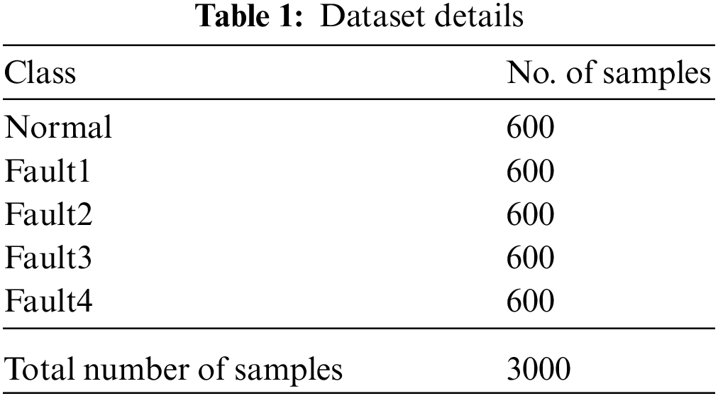
Fig. 3 highlights the confusion matrices produced by the ISOSDL-FD model on 70% of training (TR) data and 30% of testing (TS) data. With 70% of TR data, the ISOSDL-FD model has recognized 394 samples into normal, 393 samples into fault 1, 406 samples into fault 2, 400 samples into fault 3, and 405 samples into fault 4. Also, with 30% of TS data, the ISOSDL-FD method has identified 172 samples into normal, 177 samples into fault 1, 163 samples into fault 2, 171 samples into fault 3, and 172 samples into fault 4.

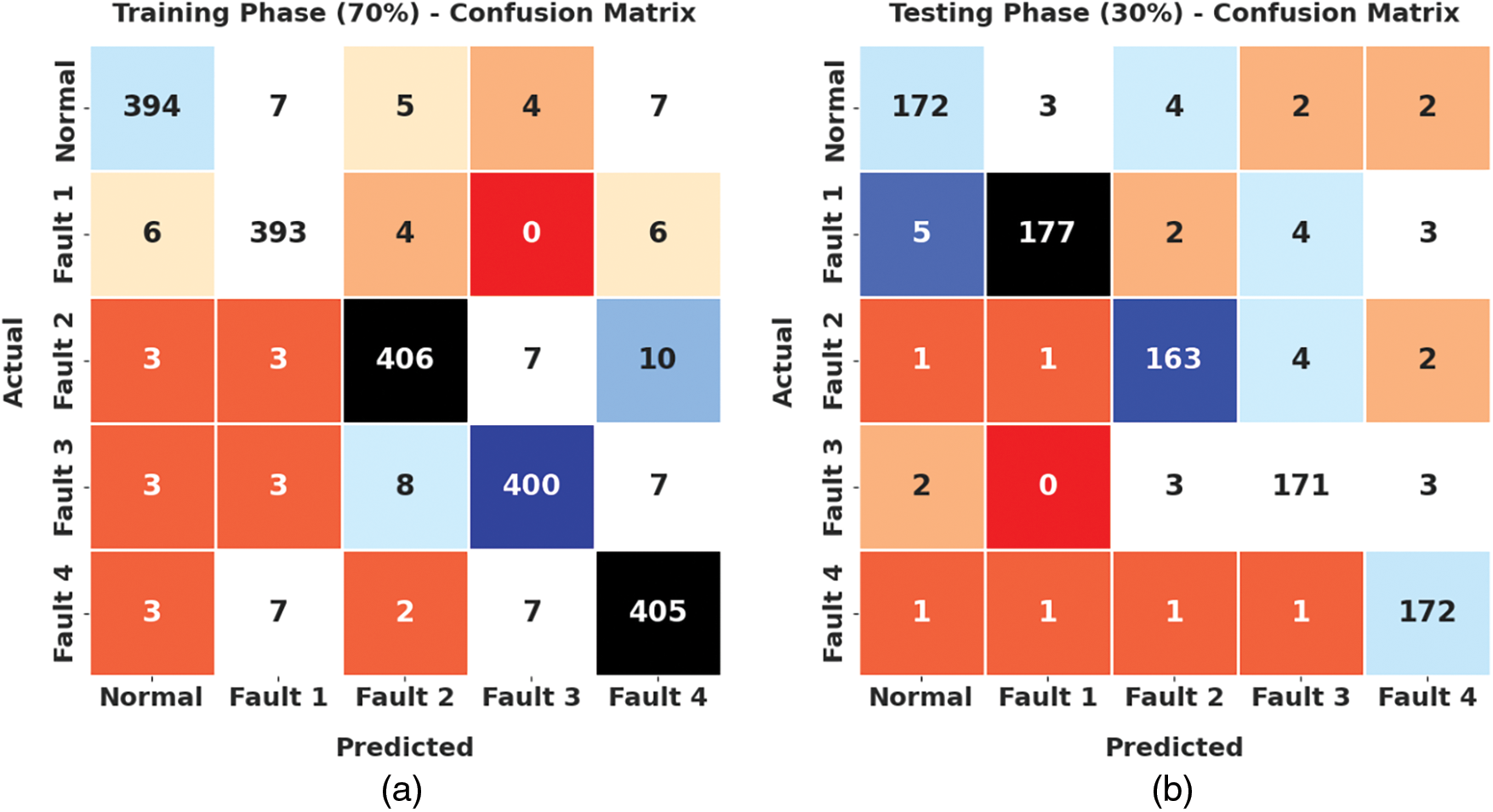
Figure 3: Confusion matrices of ISOSDL-FD approach (a) 70% of TR data and (b) 30% of TS data

Tab. 2 illustrates a detailed classification result of the ISOSDL-FD model under 70% of TR and 30% of TS data. Fig. 4 shows the result analysis of ISOSDL-FD approach under 70% of TR data. The ISOSDL-FD model has recognized normal class with accuy of 98.19%, sensy of 94.48%, specy of 99.11%, Fscore of 95.40%, MCC of 94.28%, and Gmeasure of 95.40%. Moreover, the ISOSDL-FD technique has detected Fault-1 class with accuy of 98.29%, sensy of 96.09%, specy of 98.82%, Fscore of 95.62%, MCC of 94.56%, and Gmeasure of 95.62%. Furthermore, the ISOSDL-FD technique has recognized Fault-4 class with accuy of 97.67%, sensy of 95.52%, specy of 98.21%, Fscore of 94.30%, MCC of 92.84%, and Gmeasure of 94.30%.

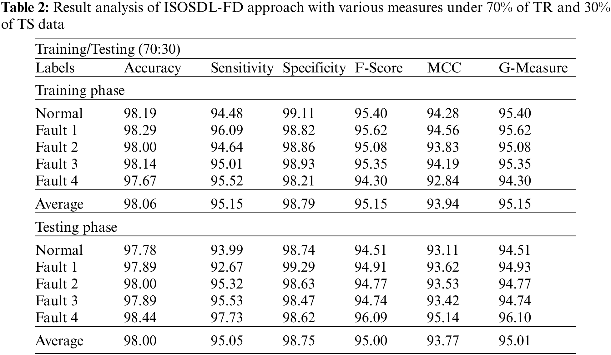
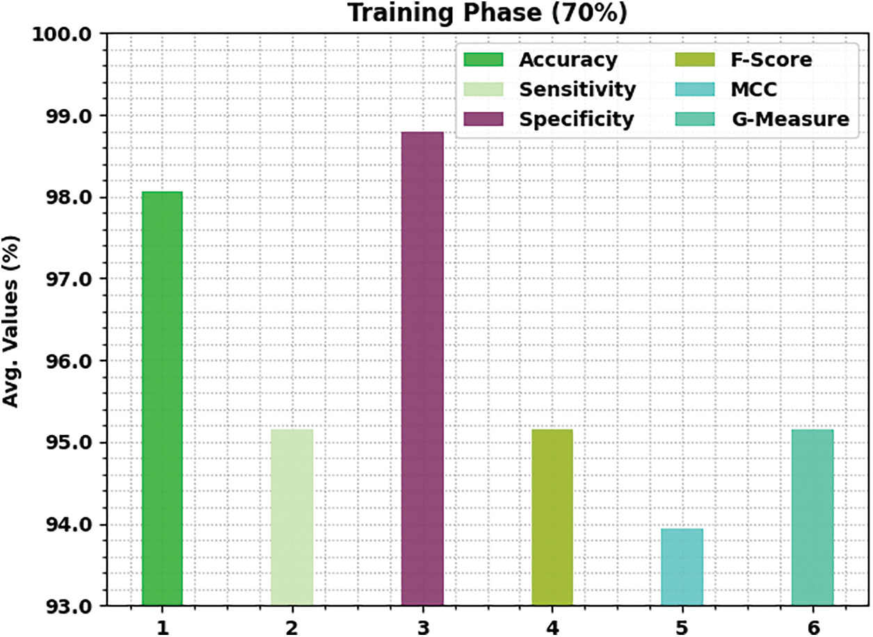
Figure 4: Average analysis of ISOSDL-FD algorithm under 70% of TR data

Fig. 5 displays the result analysis of ISOSDL-FD method under 30% of TS data. The ISOSDL-FD approach has identified normal class with accuy of 97.78%, sensy of 93.99%, specy of 98.74%, Fscore of 94.51%, MCC of 93.11%, and Gmeasure of 94.51%. in addition to that, the ISOSDL-FD methodology has recognized Fault-1 class with accuy of 97.89%, sensy of 92.67%, specy of 99.29%, Fscore of 94.91%, MCC of 93.62%, and Gmeasure of 94.93%. Also, the ISOSDL-FD technique has recognized Fault-4 class with accuy of 98.44%, sensy of 97.73%, specy of 98.62%, Fscore of 96.09%, MCC of 95.14%, and Gmeasure of 96.10%.

Figure 5: Average analysis of ISOSDL-FD algorithm under 30% of TS data

Fig. 6 exhibits the confusion matrices generated by the ISOSDL-FD approach on 80% of TR data and 20% of TS data. With 80% of TR data, the ISOSDL-FD approach has recognized 469 samples into normal, 463 samples into fault 1, 468 samples into fault 2, 470 samples into fault 3, and 466 samples into fault 4. Moreover, with 30% of TS data, the ISOSDL-FD algorithm has identified 115 samples into normal, 118 samples into fault 1, 110 samples into fault 2, 119 samples into fault 3, and 123 samples into fault 4.

Figure 6: Confusion matrices of ISOSDL-FD approach (a) 80% of TR data and (b) 20% of TS data

Tab. 3 demonstrates a brief classification result of the ISOSDL-FD method under 80% of TR and 20% of TS data. Fig. 7 displays the result analysis of ISOSDL-FD methodology under 80% of TR data. The ISOSDL-FD algorithm has recognized normal class with accuy of 99.04%, sensy of 96.90%, specy of 99.58%, Fscore of 97.61%, MCC of 97.01%, and Gmeasure of 97.61%. Furthermore, the ISOSDL-FD approach has recognized Fault-1 class with accuy of 99%, sensy of 97.27%, specy of 99.43%, Fscore of 97.47%, MCC of 96.85%, and Gmeasure of 97.47%. Also, the ISOSDL-FD method has identified Fault-4 class with accuy of 99.04%, sensy of 98.31%, specy of 99.22%, Fscore of 97.59%, MCC of 97%, and Gmeasure of 97.59%.

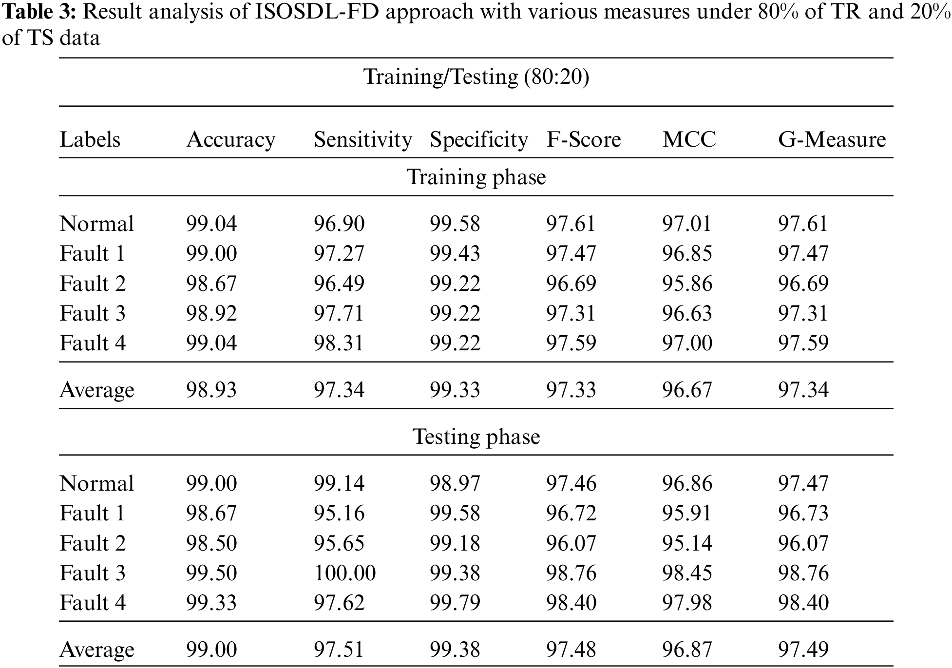
Figure 7: Average analysis of ISOSDL-FD algorithm under 80% of TR data

Fig. 8 illustrates the result analysis of ISOSDL-FD method under 20% of TS data. The ISOSDL-FD algorithm has recognized normal class with accuy of 99%, sensy of 99.14%, specy of 98.97%, Fscore of 97.46%, MCC of 96.86%, and Gmeasure of 97.47%. Additionally, the ISOSDL-FD methodology has recognized Fault-1 class with accuy of 98.67%, sensy of 95.16%, specy of 99.58%, Fscore of 96.72%, MCC of 95.91%, and Gmeasure of 96.73%. Along with that, the ISOSDL-FD technique has recognized Fault-4 class with accuy of 99.33%, sensy of 97.62%, specy of 99.79%, Fscore of 98.40%, MCC of 97.98%, and Gmeasure of 98.40%.

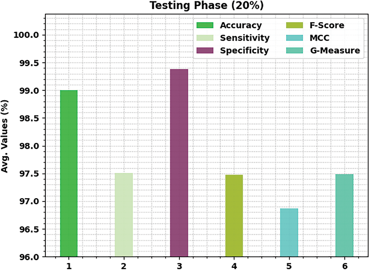
Figure 8: Average analysis of ISOSDL-FD algorithm under 20% of TS data

The training accuracy (TA) and validation accuracy (VA) acquired by the ISOSDL-FD technique on test dataset is demonstrated in Fig. 9. The experimental outcome represents the ISOSDL-FD methodology has reached higher values of TA and VA. To be specific, the VA is higher than TA.

Figure 9: TA and VA analysis of ISOSDL-FD algorithm

The training loss (TL) and validation loss (VL) gained by the ISOSDL-FD method on test dataset are established in Fig. 10. The experimental outcome indicated the ISOSDL-FD technique has accomplished minimal values of TL and VL. Particularly, the VL is lower than TL.

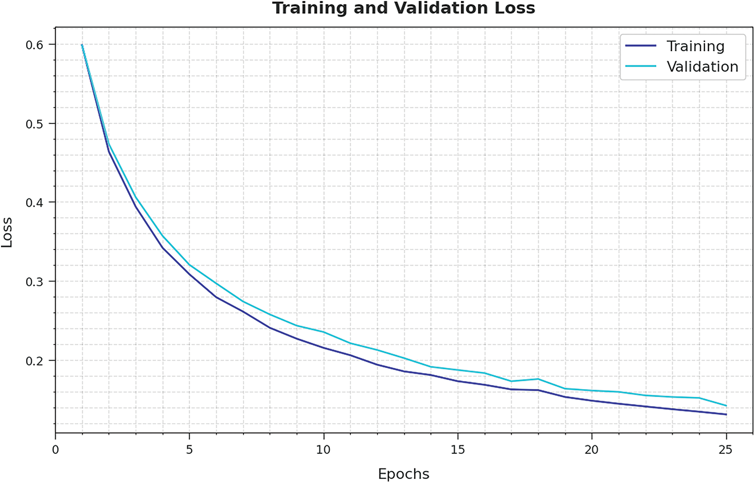
Figure 10: TL and VL analysis of ISOSDL-FD algorithm

At last, a comparative study of the ISOSDL-FD model with recent models interms of different measures is shown in Tab. 4 [22,23].

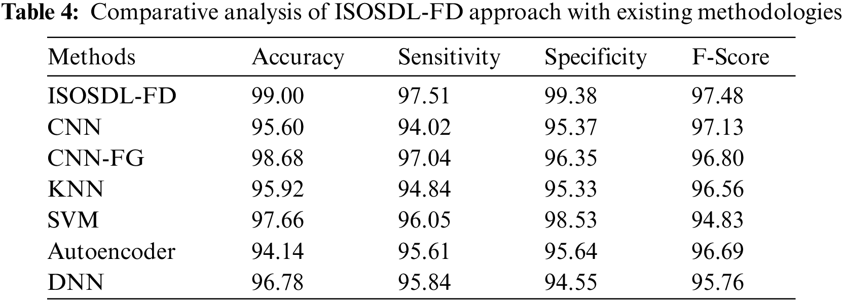
Fig. 11 inspects a detailed result analysis of the ISOSDL-FD model with existing models interms of sensy and specy. The figure implied that the ISOSDL-FD model has gained enhanced results with maximum values of sensy and specy. For instance, with respect to sensy, the ISOSDL-FD model has provided improved sensy of 97.51% whereas the CNN, CNN-FG, KNN, SVM, AE, and DNN models have resulted to reduced sensy of 94.02%, 97.04%, 94.84%, 96.05%, 95.61%, and 95.84% respectively. In addition, in connection to specy, the ISOSDL-FD method has rendered improvised specy of 99.38% whereas the CNN, CNN-FG, KNN, SVM, AE, and DNN techniques have resulted to minimal specy of 95.37%, 96.35%, 95.33%, 98.53%, 95.64%, and 94.55% correspondingly.

Figure 11: Sensyand Specy analysis of ISOSDL-FD approach with existing methodologies

Fig. 12 reviews a comparative result analysis of the ISOSDL-FD methodology with existing models interms of accuy and Fscore. The figure inferred the ISOSDL-FD technique has obtained improved results with higher values of accuy and Fscore. For example, in relation with accuy, the ISOSDL-FD approach has rendered enhanced accuy of 99% whereas the CNN, CNN-FG, KNN, SVM, AE, and DNN methods have resulted in reduced accuy of 95.60%, 98.68%, 95.92%, 97.66%, 94.14%, and 96.78% respectively. Along with that with connection with Fscore, the ISOSDL-FD model has offered improvised Fscore of 97.48% whereas the CNN, CNN-FG, KNN, SVM, AE, and DNN approaches have resulted to minimal Fscore of 97.13%, 96.80%, 96.56%, 94.83%, 96.69%, and 95.76% correspondingly.

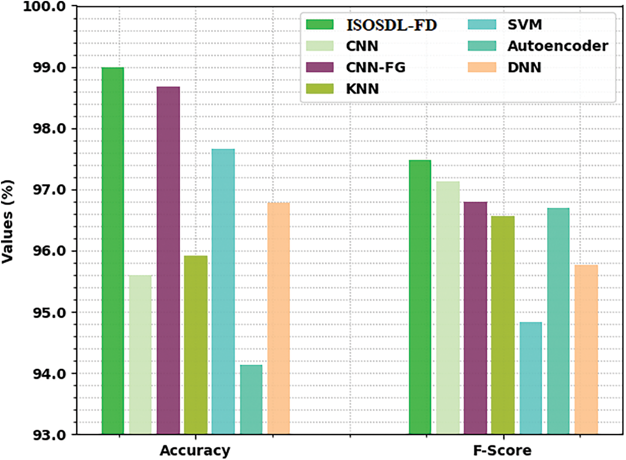
Figure 12: Accuyand Fscore analysis of ISOSDL-FD approach with existing methodologies

From the detailed results and discussion, it is apparent that the ISOSDL-FD model has shown enhanced classification performance over other models.

5  Conclusion

In this study, a new ISOSDL-FD technique was introduced for the recognition of faults in industrial systems. The proposed ISOSDL-FD technique accomplished proficient identification and classification of faults in the gearbox data. In addition, a Fast kurtogram based time-frequency analysis can be used for revealing the energy present in the machinery signals in the time and frequency representation. Moreover, the DBiRNN is applied for fault detection and classification. At last, the ISOS approach was derived for optimal hyperparameter tuning of the DL approach so that the classification performance will be improvised. To exhibit the enhanced performance of the ISOSDL-FD method, a comprehensive experimental analysis was performed. The experimental results stated the betterment of the ISOSDL-FD methodology over recent techniques with maximum accuracy of 99%. In future, the performance of the proposed model can be enhanced by the use of hybrid DL models.

Funding Statement: The author received no specific funding for this study.

Conflicts of Interest: The author declare that they have no conflicts of interest to report regarding the present study.

References

 1.  R. Liu, B. Yang, E. Zio and X. Chen, “Artificial intelligence for fault diagnosis of rotating machinery: A review,” Mechanical Systems and Signal Processing, vol. 108, pp. 33–47, 2018. [Google Scholar]

 2.  T. Zhou, T. Han and E. L. Droguett, “Towards trustworthy machine fault diagnosis: A probabilistic Bayesian deep learning framework,” Reliability Engineering & System Safety, vol. 224, pp. 108525, 2022. [Google Scholar]

 3.  Y. Qi, C. Shen, D. Wang, J. Shi, X. Jiang et al., “Stacked sparse autoencoder-based deep network for fault diagnosis of rotating machinery,” IEEE Access, vol. 5, pp. 15066–15079, 2017. [Google Scholar]

 4.  A. M. Hilal, J. S. Alzahrani, I. Abunadi, N. Nemri, F. N. Al-Wesabi et al., “Intelligent deep learning model for privacy preserving IIoT on 6G environment,” Computers, Materials & Continua, vol. 72, no. 1, pp. 333–348, 2022. [Google Scholar]

 5.  M. Kim, J. U. Ko, J. Lee, B. D. Youn, J. H. Jung et al., “A domain adaptation with semantic clustering (DASC) method for fault diagnosis of rotating machinery,” ISA Transactions, vol. 120, pp. 372–382, 2022. [Google Scholar]

 6.  M. A. Alohali, F. N. Al-Wesabi, A. M. Hilal, S. Goel, D. Gupta et al., “Artificial intelligence enabled intrusion detection systems for cognitive cyber-physical systems in industry 4.0 environment,” Cognitive Neurodynamics, 2022. https://doi.org/10.1007/s11571-022-09780-8. [Google Scholar]

 7.  Y. Ding, L. Ma, J. Ma, M. Suo, L. Tao et al., “Intelligent fault diagnosis for rotating machinery using deep Q-network based health state classification: A deep reinforcement learning approach,” Advanced Engineering Informatics, vol. 42, pp. 100977, 2019. [Google Scholar]

 8.  I. Abunadi, M. M. Althobaiti, F. N. Al-Wesabi, A. M. Hilal, M. Medani et al., “Federated learning with blockchain assisted image classification for clustered UAV networks,” Computers, Materials & Continua, vol. 72, no. 1, pp. 1195–1212, 2022. [Google Scholar]

 9.  Y. Zhang, T. Zhou, X. Huang, L. Cao and Q. Zhou, “Fault diagnosis of rotating machinery based on recurrent neural networks,” Measurement, vol. 171, pp. 108774, 2021. [Google Scholar]

10. T. Jin, C. Yan, C. Chen, Z. Yang, H. Tian et al., “Light neural network with fewer parameters based on CNN for fault diagnosis of rotating machinery,” Measurement, vol. 181, pp. 109639, 2021. [Google Scholar]

11. W. Zhang, X. Li and Q. Ding, “Deep residual learning-based fault diagnosis method for rotating machinery,” ISA Transactions, vol. 95, pp. 295–305, 2019. [Google Scholar]

12. L. C. Brito, G. A. Susto, J. N. Brito and M. A. V. Duarte, “An explainable artificial intelligence approach for unsupervised fault detection and diagnosis in rotating machinery,” Mechanical Systems and Signal Processing, vol. 163, pp. 108105, 2022. [Google Scholar]

13. W. Jiang, C. Wang, J. Zou and S. Zhang, “Application of deep learning in fault diagnosis of rotating machinery,” Processes, vol. 9, no. 6, pp. 919, 2021. [Google Scholar]

14. T. Wang, L. Zhang, H. Qiao and P. Wang, “Fault diagnosis of rotating machinery under time-varying speed based on order tracking and deep learning,” Journal of Vibroengineering, vol. 22, no. 2, pp. 366–382, 2020. [Google Scholar]

15. S. Tang, Y. Zhu and S. Yuan, “An adaptive deep learning model towards fault diagnosis of hydraulic piston pump using pressure signal,” Engineering Failure Analysis, vol. 138, pp. 106300, 2022. [Google Scholar]

16. B. Peng, H. Xia, X. Lv, M. A. Nyarko, S. Zhu et al., “An intelligent fault diagnosis method for rotating machinery based on data fusion and deep residual neural network,” Applied Intelligence, vol. 52, no. 3, pp. 3051–3065, 2022. [Google Scholar]

17. Y. Li, X. Du, F. Wan, X. Wang and H. Yu, “Rotating machinery fault diagnosis based on convolutional neural network and infrared thermal imaging,” Chinese Journal of Aeronautics, vol. 33, no. 2, pp. 427–438, 2020. [Google Scholar]

18. S. Pang, X. Yang, X. Zhang and X. Lin, “Fault diagnosis of rotating machinery with ensemble kernel extreme learning machine based on fused multi-domain features,” ISA Transactions, vol. 98, pp. 320–337, 2020. [Google Scholar]

19. S. R. Saufi, Z. A. B. Ahmad, M. S. Leong and M. H. Lim, “Gearbox fault diagnosis using a deep learning model with limited data sample,” IEEE Transactions on Industrial Informatics, vol. 16, no. 10, pp. 6263–6271, 2020. [Google Scholar]

20. O. Olabiyi, E. Martinson, V. Chintalapudi and R. Guo, “Driver action prediction using deep (bidirectional) recurrent neural network,” arXiv:1706.02257, pp. 1–7, 2017. [Google Scholar]

21. M. Y. Cheng and D. Prayogo, “Symbiotic organisms search: A new metaheuristic optimization algorithm,” Computers & Structures, vol. 139, pp. 98–112, 2014. [Google Scholar]

22. O. Essid, H. Laga and C. Samir, “Automatic detection and classification of manufacturing defects in metal boxes using deep neural networks,” PLoS One, vol. 13, no. 11, pp. e0203192, 2018. [Google Scholar]

23. P. Jiang, H. Cong, J. Wang and D. Zhang, “Fault diagnosis of gearbox in multiple conditions based on fine-grained classification cnn algorithm,” Shock and Vibration, vol. 2020, pp. 1–15, 2020. [Google Scholar]