Automated Deep Learning Driven Crop Classification on Hyperspectral Remote Sensing Images

1  Introduction

With the technological advancement in remote sensing image (RSI) acquisition mechanism and the greater accessibility of rich spatial and spectral datasets through a collection of sensors, hyperspectral imaging technique has become increasingly important. Particularly, Hyperspectral Image (HSI) classification has become a great source for real-time application in fields such as forestry, environment, mineral mapping, agriculture, and so on [1]. HSI classification (assigning all the pixels to one specific class depending upon their spectral features) was a most active research topic in the HSI and attracted considerable attention in the remote sensing fields [2]. In HSI classification task, there are 2 major challenges one is the limited available training samples against the high dimensionalities of hyperspectral data and another one is the large spatial variability of spectral signs. Initially, it is often brought by several components including variations in environmental, illumination, temporal, and atmospheric conditions [3]. Next, it results in ill posed problems for certain techniques and minimizes the generalizing capability of classification.

Conventional technique obtains crop classification outcomes by using field investigation, statistics, and measurement, which are money-consuming, time-taking, and labor-consuming [4]. Remote sensing technique advanced by bounds and leaps, timeliness and resolution of RSI has been developed, and hyperspectral remote sensing information is extensively applied [5,6]. In particular, hyperspectral information plays a significant role in agricultural surveys and is utilized for agricultural yield estimation, pest monitoring, crop condition monitoring, etc. In agriculture surveys, the fine classifying of HIS provide the data on crop distribution [7]. Fine classifying of crop needs image with higher spectral and spatial resolution. In recent times, as a significant part of machine learning, deep learning (DL) has gained considerable attention as a result of its stronger abilities in feature extraction and analysis [8]. By extracting features of the input dataset from the bottom to the top of the networks, DL model forms the higher-level abstract feature appropriate for pattern categorization [9].

Out of several DL methods, a convolutional neural network (CNN) contains a comparatively smaller amount of weights due to sharing weights and local connections [10]. A quantity of DL structures was suggested and admired by neuro-science researchers. The CNN is regarded as an unusual case of deep neural networks (DNN) which are advanced for processing images but also utilized for other kinds of data such as audio [11]. It could scan multi-dimensional input piece-by-piece with a convolutional window that means a neuron set having typical weights. The output respective to single convolutional window was known as a feature map and was taken as a map of activities of a provided feature over entire inputs [12]. The CNN serves as one such most famous architectures for DLNN categorization in recent times.

This article presents a novel Hurricane Optimization Algorithm with Deep Transfer Learning Driven Crop Classification (HOADTL-CC) model on Hyperspectral RSIs. The presented HOADTL-CC model uses HOA with capsule network (CapsNet) model for generating useful feature vectors set. Moreover, Elman neural network (ENN) model is applied to allot proper class labels into the input HSI. Lastly, glowworm swarm optimization (GSO) algorithm is exploited to fine tune the ENN parameters involved in this paper. The experimental result examination of the HOADTL-CC approach can be tested with the use of a benchmark dataset.

2  Literature Review

Bhosle et al. [13] examine an estimation of CNN for crop classifier utilizing the Indian Pines standard dataset attained in the AVIRIS sensor and the research region dataset reached in the EO-1hyperion sensor. An optimization CNN was adapted by training the method on distinct parameters. It is related to 2 classifier techniques such as DNN and Convolutional Auto-encoder (AE). The author [14] utilizes a new 3D deep CNN (DCNN) technique which directly integrates the hyperspectral information. Besides, the authors examine the learned method for producing physiologically meaningful clarifications. The authors concentrate on an economically vital disease, charcoal rot that is a soil borne fungal disease which affected the yield of soybean crops worldwide. In [15], the morphological profiles, GLCM texture, and endmember abundance features were leveraged for exploiting the spatial data of HSI. Afterward, several spatial data were fused with original spectral data for generating classifier outcomes by utilizing the DNN with conditional random field (DNN+CRF) approach. Especially, the DNN is a deep detection method that is extracting depth features and mine the potential data. As a discriminant method, the CRF assumes both spatial as well as contextual data for reducing the misclassified noises while holding the object boundary.

In [16], the authors provide a distinct viewpoint on solving the hyperspectral pixel-level classifier tasks. The recent approaches employ difficult methods for this task, however, the efficacy of these approaches is frequently ignored. According to this observation, the authors present an effectual small method for spectral-spatial classifier on HSIs dependent upon a single gated recurrent unit (GRU). During this method, an essential GRU is learned spectral correlation in an entire spectrum input, and spatial data are fused as the primary hidden state of GRU. Han et al. [17] present minimum redundancy and maximum relevance (mRMR) FS approach for directly choosing important raw bands in HSIs. Besides, a DNN was offered for classifying the hyperspectral information with decreased dimensional that contains CNN than a fully connected network (FCN). In [18], a quick and non-destructive approach utilizing HSI coupled with DL classifier has been executed to the quality estimate of unblanched kernel from Canarium indicum classified by peroxide value (PV). The group of 2300 sub-images of 289 C. indicum instances was utilized for training a CNN for estimating quality level.

3  The Proposed Model

In this study, a new HOADTL-CC approach was advanced for the identification and categorization of crops on the hyperspectral RSIs. The proposed HOADTL-CC model incorporates a series of processes namely CapsNet feature extractor, HOA based hyperparameter optimizer, ENN classification, and GSO based parameter optimization. Here, the GSO algorithm is exploited to fine tune the ENN parameters involved in this study. Fig. 1 depicts the block diagram of HOADTL-CC approach.

Figure 1: Block diagram of HOADTL-CC approach

3.1 Feature Extraction

In this study, the CapsNet model is used to generate a set of useful feature vectors. A CapsNet is a new form of CNN which aims at providing data regarding the presence or spatial relationships of features (scales, locations, orientations, brightness, and so on.) in an image [19]. The basis of network depends on the addition of concept named “capsules”. A capsule is a set of neurons that include probability of certain object presence and useful value related to instantiation parameters including pose, rotation, slope, posture, direction, position, scale, and thickness. Different from CNN modules such as convolution and pooling that cause data loss, capsules can able to hold further details.

Fig. 2 depicts the structure of CapsNet method. The novelty in CapsNets is the “routing by agreement” concept that can be replaced by pooling. Based on these concepts, output is transferred to each parent capsule in the next layer, but the coupling coefficient is not the same. All the capsules try to evaluate the output of parental capsule, and if this estimate matches the original output of parental capsule, the coupling coefficients among the two capsules rise. Consider ui as the output of ithcapsules, their prediction for jth parental capsules are evaluated by

u^j|i=Wijui(1)

Figure 2: Structure of CapsNet

In Eq. (1), u^j|i refers to the predictive vector of the output of j-th capsules at a high level calculated using i-th capsules, and Wij denotes the weighting matrix that should be learned in the backward pass. According to the degree of confirmation among the capsules and the parental capsules, cij coupling coefficient is evaluated by the subsequent softmax function

cij=exp⁡(bij)Σkexp⁡(bij)(2)

In Eq. (2), bij represents the log likelihood that capsule i needs to be combined with jth capsules and set to zero. Therefore, the input vector to parental capsule j is calculated by using the Eq. (3)

sj=∑iaj⋅u^j|i(3)

At last, the no-linear squashing function is utilized for preventing the output vector of capsule from above one and form the last output of every capsule as follows

θj=‖sj||21+‖sj‖2sj‖sj‖(4)

The new framework accomplishes considerably better, current performance accuracy with MNIST dataset.

To summarize the capsule network process, the capsule determines the feature parameter in certain objects. In the object identification process, capsule determines the absence or presence of an object and considers the corresponding parameter, where the object feature is organized. This implies the method identifies the object once the feature identified by capsule is existing in the correct sequence. The working process of the capsule is given below:

•   Initially, capsule proceeds with the matrix multiplication of input vector with weight matrix that characterize the spatial relationship of lower-level feature with higher-level feature;

•   Capsule decides the parental capsules. This can be accomplished by the dynamic routing algorithm. For instance, the system tries to identify an image of a house from diverse perspectives. Capsule extracts the data regarding the walls and roof, but this doesn’t mean any roof can be a house. As a result, the capsule analyzes the reliable part in the image. To decide whether the object is a house (or else), prediction is made by using roofs and walls. Such predictions are later transferred to the high-level capsules. Once the prediction is right, the object is allocated as a house;

•   Afterward the parent capsule decision, the process proceeds by summing each vector eventually squashed to 0 and 1 while preserving the direction. Squashing can be done by norm calculation as the probability of presence and cosine distance as a degree of agreement.

3.2 HOA Based Parameter Tuning

To adjust the hyperparameters [20–22] indulged in the CapsNet model, the HOA was utilized. The HOA follows the communication of the natural forces of hurricanes and wind parcels initiate there, making them for moving nearby the distinct regions of hurricane [23]. The HOA work with primary population collected by wind parcels arbitrarily distributed from the hurricane, this permits the technique for starting with their exploration as well as exploitation procedures from the solution spaces. A primary population of wind parcels gets the infrastructure demonstrated in Eq. (5):

Pt=[p11tp12t⋯p1Nvtp21tp22t⋯p2Nvt⋮⋮⋱⋮pNi1tpNi2t⋯pNi,Nvt](5)

whereas Pt refers the wind parcels population from the iteration t, if t=0 the primary population of individuals is attained. Ni signifies the amount of wind parcels (individuals) and Nv denotes the amount of variables or the dimensional of solution spaces, conversely, the amount of parameters of a single phase transformer.

For creating the primary population of individuals it can be utilized in Eq. (6) that creates a matrix of arbitrary numbers in the upper as well as lower limits which comprises feasible solution to problem in this case.

P0=yminones(Ni,Nv)+(ymax−ymin)rand(Ni,Nv)(6)

whereas ones (Ni,Nv)∈RNi×Nv implies the all-ones matrix. rand(Ni,Nv)∈RNi×Nv indicates the all-random numbers matrix in [0, 1] created in a normal distribution. At last, ymin∈Rdim×1yymax∈RNv×1 were vectors which signify the upper as well as lower limits of solution spaces. Because of the communication of wind parcels with natural force of hurricanes, it can be displaced from its primary point to distinct point of solution spaces. This movement is demonstrated mathematically in 2 distinct approaches because of rotation offered by hurricane winds as demonstrated in Eqs. (7) and (8).

Pit+1={ritsin(ϕi0+ϕit)+PHEtr1<0.5ritcos(ϕi0+ϕit)+PHEtr1≥0.5(7)

rit=R0exp(r2ϕit)(8)

In which Pit+1 signifies the novel place of wind parcels i if the evolution condition of the technique was executed, being i=1,2,…,Ni.

The parameter r1 are an arbitrary variable amongst zero and one that ensures the equity of commuting among the sine and cosine trigonometric functions referred to in Eq. (7). ϕi0 implies the primary angular co-ordinate of wind parcels i that gets arbitrary values amongst [0, 2π]. PHEt denotes the hurricane eye from the iteration t. rit and ϕit signifies the radial and angular coordinates from polar representation correspondingly. In Eq. (8) if t=0,ϕit is an all-zeros vector, where rit is obtain the value of R0. Being R0 the radius of hurricane eye that gets the value of 1×10−5. Eventually, r2 demonstrates the arbitrary number amongst zero and one. While the wind parcel Pit+1 requires the velocity for starting move and keep in the movement, it can be assumed that change rate from the angular displacement (angular velocity) summed to their angular co-ordinate ϕit, as depicted in Eq. (9).

ϕit+1={ϕit+writ≤Rmaxϕit+w(Rmaxrit)r3rit>Rmax(9)

whereas, w represents the angular velocity that is considered constant with value of π10 and Rmax is the radius whereas the maximal wind velocity was established that is obtained as 0.2. Lastly, r3 signifies the arbitrary value amongst zero and one. For making the solutions possible, novel places of wind parcels produced by communication of hurricane forces, take that in the limit of solution spaces.

In this sense, the upper as well as lower limits were confirmed for all the individuals restricted from the group of novel places Pt+1, as displayed in Eq. (10).

Pit+1={Pit+1ymin≤Pit+1≤ymaxymin+rand(ymax−ymin)otherwise(10)

whereas rand offers arbitrary numbers with normal distribution amongst zero and one. Some individuals in the group of candidate solutions Pt+1 is chosen as the novel hurricane eye if, and only if, the value of their objective function was superior to the present hurricane eye PHEt. This upgrade was determined in Eq. (11).

PHEt+1={Pit+1IfF(Pit+1)<F(PHEt)PHEtotherwise(11)

whereas F(⋅) implies the objective function.

3.3 Optimal ENN Based Classification

Once the feature vectors are derived, the next stage is the classification process using the ENN model. Elman proposed an ENN was the standard local recursion delay FFNN [24]. The ENN adds a context layer as internal feedback according to BPNN and also it could store state data. Especially, ENN stores the output values of hidden state at t time in the context layers, the input of hidden state at T+1 time includes the input of the hidden state at T+1 time, and the output of hidden layer at t time. Consequently, ENN is very suitable for determining time series predictive method. The mathematical expression of ENN is given below:

{x(k)=f(w3xc(k)+w1u(k−1))xc(k)=αxc(k−1)+x(k−1)y(k)=g(w2x(k))(12)

In Eq. (12), u refers to the input value, the k represents at k-th iteration steps. w1, w2 and w3 denotes the connection weight of input to the hidden layers, the hidden to output layers, and context to hidden layers, correspondingly. b1, b2 and b3 indicates the threshold of the hidden, output, and context layers, correspondingly. α refers to self-connected feedback gain factor. The activation function of hidden state utilized the sigmoid function and the linear function was utilized as activation function for the output layer. y(k) indicates the target output.

For effectual adjustment of the ENN parameters, the GSO algorithm has been exploited. Here, a set of glowworms is distributed and initialized in a random manner from the solution space [25]. The intensity of emitted light was associated with the luciferin count, i.e., strongly associated with it, while the glowworm was situated from the movement and had a dynamic decision range rdi(t) constraint using a spherical sensor range rs(0<rdi<=rsi). At first, the glowworm encompasses an equal number of luciferins, l0. According to the similarity of luciferin value, the i glowworm chooses their neighboring one j with pij possibility and shift from the direction of decision range rs(0<rdi<=rsi), while the location of the glowworm i is characterized as xi(xi∈Rm,i=1,2,…,n).

A luciferin update phase is impacted using the function value in the glowworm position:

li(t+1)=(1−ρ)li(t)+γJ(xi(x+1))(13)

In Eq. (13), li(t) indicates the luciferin level interconnected with a glowworm i at time t, ρ denotes the luciferin decay constant 0<ρ<1, γ indicates the luciferin constant, and J(xi(t)) indicates the value of major function at agent i-th location at time t.

Also, in the process included in the GSO approach, glowworm is fascinated using the neighbor that glows brightly. Therefore, the results during the movement stage, the glowworms use the probabilistic method for moving toward the neighbor that has a maximal luciferin intensity. Especially for every i glowworms, the moving possibility over a neighborhod glowworm is denoted by:

pij(t)=lj(t)−lj(t)Σk∈Ni(t)lk(t)−li(t)(14)

In Eq. (14), j∈Ni(t), Ni(t)={j:dij(t)<rdi(t),li(t),li(t)<lj(t)} embodies the set of neighboring glowworms i at time t, dij(t) refers to the Euclidean distance among the i and j glowworms at time t, rdi(t) indicates the parameter neighboring range associated with i glowworm at t time. The parameter controlled by a radial sensor ranges from (0<rdi<rs).

xi(t+1)=xi(t)+s[xj(t)−xi(t)||xj(t)−xi(t)||](15)

In Eq. (15), s(>0) indicates the step size, and |||| denotes the Euclidean norm operator. Furthermore, xi(t)∈Rm denotes the position of i glowworm at t time from m dimension real space Rm. Then, consider r0 represent the initialized neighborhood range of each glowworm (i.e., rdi(0)=r0, ∀i):

rdi(t+1)=min{rs,max{0,rdi(t)+β(nr−|Ni(t)|)}}(16)

In Eq. (16) β refers to a constant, and nt determines a variable employed for controlling the degree.

The GSO system develops a fitness function (FF) for achieving superior classifier efficiency. It defines a positive integer for representing the best efficiency of candidate solutions. During this case, the minimized classifier error rate was supposed that FF is providing in Eq. (17).

fitness(xi)=ClassifierErrorRate(xi)=numberofmisclassifiedsamplesTotalnumberofsamples∗100(17)

4  Result and Discussion

In this section, the experimental validation of the suggested method was carried out against dataset-1 [26] (WHU-Hi-LongKou). It comprised total of 9,000 samples with 9 class labels, holding 1000 samples under every class as shown in Tab. 1. Fig. 3 depict the sample HSIs from various classes involved in dataset 1.

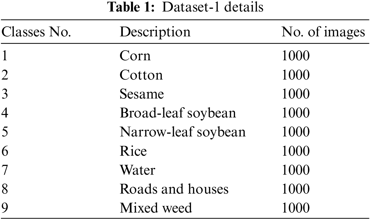
Figure 3: Sample images on dataset-1

Fig. 4 showcases the confusion matrix offered by the HOADTL-CC model on dataset-1. The figure implied that the HOADTL-CC model has proficiently recognized 985 samples into class 1, 983 samples into class 2, 963 samples into class 3, 990 samples into class 4, 991 samples into class 5, 979 samples into class 6, 979 samples into class 7, 946 samples into class 8, and 986 samples into class 9.

Figure 4: Confusion matrices of HOADTL-CC approach on dataset-1

A brief crop classifier outcome of the presented HOADTL-CC model on dataset-1 is demonstrated in Tab. 2 and Fig. 5. The results indicated that the presented HOADTL-CC model has shown effectual results under every class label. For instance, the HOADTL-CC model has recognized images under corn class with accuy of 99.50%, recal of 98.50%, specy of 99.62%, and Fscore of 97.77%. Meanwhile, the HOADTL-CC technique has recognized images under rice class with accuy of 99.69%, recal of 97.90%, specy of 99.91%, and Fscore of 98.59%. Eventually, the HOADTL-CC approach has recognized images under mixed weed class with accuy of 99.76%, recal of 98.60%, specy of 99.90%, and Fscore of 98.90%.

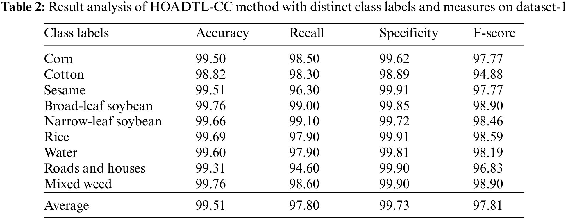
Figure 5: Average analysis of HOADTL-CC method with distinct class labels on dataset-1

The training accuracy (TA) and validation accuracy (VA) gained by the HOADTL-CC method on dataset-1 is established in Fig. 6. The experimental outcome revealed that the HOADTL-CC approach has acquired maximum values of TA and VA. In specific, the VA is performed that higher than TA.

Figure 6: TA and VA analysis of HOADTL-CC algorithm on dataset-1

The training loss (TL) and validation loss (VL) obtained by the HOADTL-CC system on dataset-1 are recognized in Fig. 7. The experimental outcome represented that the HOADTL-CC methodology has accomplished least values of TL and VL. In specific, the VL appeared to be lower than TL.

Figure 7: TL and VL analysis of HOADTL-CC algorithm on dataset-1

A brief precision-recall examination of the HOADTL-CC model under dataset-1 is portrayed in Fig. 8. By observing the figure, it is noticed that the HOADTL-CC model has accomplished maximum precision-recall performance under all classes.

Figure 8: Precision-recall curve analysis of HOADTL-CC algorithm on dataset-1

To ensure the enhanced performance of the HOADTL-CC model, a comparative analysis with existing methods [27] on dataset-1 is made in Tab. 3 and Fig. 9. The figure demonstrated that the SVM, FNEA-OO, and SVRFMC models have obtained lower accuy of 96.18%, 97.57%, and 97.99% respectively. Besides, the CNN and CNN-CRF models have attained closer accuy values of 98.38% and 98.94% respectively. However, the HOADTL-CC model has shown effectual performance over other models with maximum accuy of 99.51%.

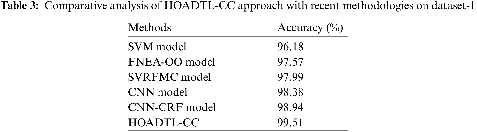
Figure 9: Comparative analysis of HOADTL-CC approach on dataset-1

5  Conclusion

In this study, a new HOADTL-CC model was advanced for the identification and categorization of crops on the hyperspectral RSIs. The proposed HOADTL-CC model includes a series of processes namely CapsNet feature extractor, HOA based hyperparameter optimizer, ENN classification, and GSO based parameter optimization. Here, the GSO algorithm is exploited to fine tune the ENN parameters involved in this study. The experimental result scrutiny of the HOADTL-CC method was tested with the help of a benchmark dataset and the results are assessed under distinct aspects. The extensive comparative studies stated the enhanced performance of the HOADTL-CC model over recent approaches. Thus, the presented HOADTL-CC model can be exploited as an effectual tool to classify crops. In future, ensemble of DL based fusion methods can be applied to boost the classification results.

Funding Statement: The authors extend their appreciation to the Deanship of Scientific Research at King Khalid University for funding this work through Large Groups Project under Grant Number (25/43). Princess Nourah bint Abdulrahman University Researchers Supporting Project Number (PNURSP2022R303), Princess Nourah bint Abdulrahman University, Riyadh, Saudi Arabia. The authors would like to thank the Deanship of Scientific Research at Umm Al-Qura University for supporting this work by Grant Code: 22UQU4340237DSR28.

Conflicts of Interest: The authors declare that they have no conflicts of interest to report regarding the present study.

References

1. N. Audebert, B. L. Saux and S. Lefèvre, “Deep learning for classification of hyperspectral data: A comparative review,” IEEE Geoscience and Remote Sensing Magazine, vol. 7, no. 2, pp. 159–173, 2019. [Google Scholar]
2. X. Ma, H. Wang and J. Wang, “Semisupervised classification for hyperspectral image based on multi-decision labeling and deep feature learning,” ISPRS Journal of Photogrammetry and Remote Sensing, vol. 120, pp. 99–107, 2016. [Google Scholar]
3. K. Nagasubramanian, S. Jones, A. K. Singh, S. Sarkar, A. Singh et al., “Plant disease identification using explainable 3D deep learning on hyperspectral images,” Plant Methods, vol. 15, no. 1, pp. 1–10, 2019. [Google Scholar]
4. G. Polder, P. M. Blok, H. A. D. Villiers, J. M. V. D. Wolf and J. Kamp, “Potato virus Y detection in seed potatoes using deep learning on hyperspectral images,” Frontiers in Plant Science, vol. 10, pp. 209, 2019. [Google Scholar]
5. I. Abunadi, M. M. Althobaiti, F. N. Al-Wesabi, A. M. Hilal, M. Medani et al., “Federated learning with blockchain assisted image classification for clustered UAV networks,” Computers, Materials & Continua, vol. 72, no. 1, pp. 1195–1212, 2022. [Google Scholar]
6. M. K. Shahvandi, “Accuracy assessment of crop classification in hyperspectral imagery using very deep convolutional neural networks,” in Second Int. Congress on Science and Engineering, Paris, France, pp. 1–10, 2020. [Google Scholar]
7. A. M. Hilal, H. Alsolai, F. N. A. Wesabi, M. K. Nour, A. Motwakel et al., “Fuzzy cognitive maps with bird swarm intelligence optimization-based remote sensing image classification,” Computational Intelligence and Neuroscience, vol. 2022, pp. 1–12, 2022. [Google Scholar]
8. C. Nguyen, V. Sagan, M. Maimaitiyiming, M. Maimaitijiang, S. Bhadra et al., “Early detection of plant viral disease using hyperspectral imaging and deep learning,” Sensors, vol. 21, no. 3, pp. 742, 2021. [Google Scholar]
9. V. I. Kozik and E. S. Nezhevenko, “Classification of hyperspectral images using conventional neural networks,” Optoelectronics, Instrumentation and Data Processing, vol. 57, no. 2, pp. 123–131, 2021. [Google Scholar]
10. A. Khan, A. D. Vibhute, S. Mali and C. H. Patil, “A systematic review on hyperspectral imaging technology with a machine and deep learning methodology for agricultural applications,” Ecological Informatics, vol. 69, pp. 101678, 2022. [Google Scholar]
11. P. D. Dao, Y. He and C. Proctor, “Plant drought impact detection using ultra-high spatial resolution hyperspectral images and machine learning,” International Journal of Applied Earth Observation and Geoinformation, vol. 102, pp. 102364, 2021. [Google Scholar]
12. B. Scherrer, J. Sheppard, P. Jha and J. A. Shaw, “Hyperspectral imaging and neural networks to classify herbicide-resistant weeds,” Journal of Applied Remote Sensing, vol. 13, no. 4, pp. 1, 2019. [Google Scholar]
13. K. Bhosle and V. Musande, “Evaluation of CNN model by comparing with convolutional autoencoder and deep neural network for crop classification on hyperspectral imagery,” Geocarto International, vol. 37, no. 3, pp. 813–827, 2022. [Google Scholar]
14. L. Wei, K. Wang, Q. Lu, Y. Liang, H. Li et al., “Crops fine classification in airborne hyperspectral imagery based on multi-feature fusion and deep learning,” Remote Sensing, vol. 13, no. 15, pp. 2917, 2021. [Google Scholar]
15. E. Pan, X. Mei, Q. Wang, Y. Ma and J. Ma, “Spectral-spatial classification for hyperspectral image based on a single GRU,” Neurocomputing, vol. 387, pp. 150–160, 2020. [Google Scholar]
16. K. Park, Y. K. Hong, G. H. Kim and J. Lee, “Classification of apple leaf conditions in hyper-spectral images for diagnosis of Marssonina blotch using mRMR and deep neural network,” Computers and Electronics in Agriculture, vol. 148, pp. 179–187, 2018. [Google Scholar]
17. Y. Han, Z. Liu, K. Khoshelham and S. H. Bai, “Quality estimation of nuts using deep learning classification of hyperspectral imagery,” Computers and Electronics in Agriculture, vol. 180, pp. 105868, 2021. [Google Scholar]
18. A. Shahroudnejad, P. Afshar, K. N. Plataniotis and A. Mohammadi, “Improved explainability of capsule networks: Relevance path by agreement,” in 2018 IEEE Global Conf. on Signal and Information Processing (GlobalSIP), Anaheim, CA, USA, pp. 549–553, 2018. [Google Scholar]
19. B. C. Caicedo, O. D. Montoya and A. A. Londoño, “Application of the hurricane optimization algorithm to estimate parameters in single-phase transformers considering voltage and current measures,” Computers, vol. 11, no. 4, pp. 55, 2022. [Google Scholar]
20. K. Shankar, E. Perumal, M. Elhoseny and P. T. Nguyen, “An IoT-cloud based intelligent computer-aided diagnosis of diabetic retinopathy stage classification using deep learning approach,” Computers, Materials & Continua, vol. 66, no. 2, pp. 1665–1680, 2021. [Google Scholar]
21. A. F. S. Devaraj, G. Murugaboopathi, M. Elhoseny, K. Shankar, K. Min et al., “An efficient framework for secure image archival and retrieval system using multiple secret share creation scheme,” IEEE Access, vol. 8, pp. 144310–144320, 2020. [Google Scholar]
22. M. Elhoseny, M. M. Selim and K. Shankar, “Optimal deep learning based convolution neural network for digital forensics face sketch synthesis in internet of things (IoT),” International Journal of Machine Learning and Cybernetics, vol. 12, no. 11, pp. 3249–3260, 2021. [Google Scholar]
23. Y. Zhang, J. Zhao, L. Wang, H. Wu, R. Zhou et al., “An improved OIF elman neural network based on CSO algorithm and its applications,” Computer Communications, vol. 171, pp. 148–156, 2021. [Google Scholar]
24. Y. Xiuwu, L. Qin, L. Yong, H. Mufang, Z. Ke et al., “Uneven clustering routing algorithm based on glowworm swarm optimization,” Ad Hoc Networks, vol. 93, pp. 101923, 2019. [Google Scholar]
25. Y. Zhong, X. Hu, C. Luo, X. Wang, J. Zhao et al., “WHU-Hi: UAV-borne hyperspectral with high spatial resolution (H2) benchmark datasets and classifier for precise crop identification based on deep convolutional neural network with CRF,” Remote Sensing of Environment, vol. 250, pp. 112012, 2020. [Google Scholar]
26. M. Jain, V. Singh and A. Rani, “A novel nature-inspired algorithm for optimization: Squirrel search algorithm,” Swarm and Evolutionary Computation, vol. 44, pp. 148–175, 2019. [Google Scholar]
27. Y. Zhong, X. Wang, Y. Xu, S. Wang, T. Jia et al., “Mini-UAV-borne hyperspectral remote sensing: From observation and processing to applications,” IEEE Geoscience and Remote Sensing Magazine, vol. 6, no. 4, pp. 46–62, 2018. [Google Scholar]
Cite This Article
Copyright © 2023 The Author(s). Published by Tech Science Press.
This work is licensed under a Creative Commons Attribution 4.0 International License , which permits unrestricted use, distribution, and reproduction in any medium, provided the original work is properly cited.
Downloads
Citation Tools