Hybrid Models for Breast Cancer Detection via Transfer Learning Technique

1  Introduction

Breast cancer has plays a vital role in touching the female mortality today and is one of the most often diagnosed malignancies which has the highest prevalence among women in the globe according to cancer data [1]. So, the early breast detection is still the foundation of breast cancer control, according to WHO research [2], which can enhance the prognosis and survival rate of breast cancer patients. This disease starts its activity in the breast cells of both men and women. In addition to this, Cancer begins in cells and spreads to other parts of the human being and the additional cell growth develops a bulk of tissue named as a lump. For example, it is the second most frequent type of cancer in the world, after lung cancer, and the fifth most common cause of cancer-related death.

Researchers from all over the world are actively collaborating and attempting to create early detection methods for breast cancer, and to solve this issue, various cutting-edge technologies have contributed in this arena, reducing the mortality rate due to breast cancer [3]. Because of their structure, size, and location, automatically locating and identifying cancer cells is a difficult challenge today. Therefore, contribution of developing a robust method for early detection of cancer will be highly appreciated. Moreover the Mammography is a preclusive screening test for breast cancer detection. The cause of Breast cancer is still an open area of research. Its treatment is very expensive and patients go through several levels of pain.

Regular check-ups for the early detection are the only cure of this disease and in advanced stages it becomes very challenging for the doctors to save the patents. At the early stage, two strategies for cancer detection are: The first is Early Diagnosis, which aims to raise the proportion of breast cancers detected at an early stage, allowing for treatment that is more effective and lowering the risk of mortality from breast cancer. The second is screening, which is a method of evaluating women even before cancer symptoms appear. This method does the rectification of cancer using various tools such as: Breast self-exam (BSE), Clinical breast exam (CBE) and the Mammography [4].

For many years, neural networks [5–8] have been investigated, and they have recently made significant advances in the field of computer vision [9]. Deep neural network (DNN) models outperform standard machine learning models, especially when it comes to analyzing big annotated datasets [10–15]. DNNs, in contrast to typical machine learning models, can extract deep features from the original input images, which are hidden and yet contain a lot of information. However, the system’s efficiency and accuracy decrease as a result of the complexity of typical machine learning procedures such as pre-processing, segmentation, feature extraction, and others. The system’s efficiency and accuracy suffer. The Deep Learning (DL) approach can be used to overcome traditional machine learning (ML) problems which has just appeared recently.

Recently it is observed that Convolution Neural Network (CNNs) are the most prevalent DL algorithms which are proposed in the literature. Image classification using convolution neural networks (CNNs) has made significant progress recently. The advent of CNN challenged the field of medical image processing, and research in this area used deep models to push the system’s performance to never-before-seen levels. The 2D input-image structure is used to modify the CNN architecture [16], A CNN-training assignment necessitates a huge amount of data, which is in short supply in the medical field, particularly in breast cancer (BC). There have been a number of reported cases when CNNs have produced good outcomes [17–19]. They do, however, have some limits. CNNs require a huge number of labelled images which is particularly troublesome given the time it takes to train a big CNN.

The rationale here is supported by past literature, such as [20,21] where many writers have suggested that fine-tuning, as well as employing a pre-trained model, could increase the system’s overall performance. So, solution is to use the Transfer Learning (TL) approach using a natural-images dataset, such as ImageNet, then apply a fine-tuning technique to solve this problem. By merging the information of individual CNN designs, the TL concept can be used to improve their performance [22]. The main benefit of TL is that it improves classification accuracy and speeds up the training process. A model transfer is a good TL strategy since the network parameters are first pre-trained using the source data, then applied in the target domain, and finally adjusted for better performance.

Transfer learning is a framework that train the architecture in one area called as (source) and then applies what it has learnt in the other domain called as (target). This, of course, offers a number of advantages: 1) training time is lowered greatly; 2) the problem of imbalanced class classification is largely resolved. The learnt parameters are then transferred to the BC-classification task using a pre-trained CNN such as the inception V3, VGG19, VGG16, ResNet50, and InceptionV2 ResNet [23–25]. The main goals of this work is to use segmentation to automatically remove the damaged patch, reduce training time, and enhance classification performance.

Motivation

Today one of the most commonly diagnosed solid malignancies is the breast cancer and the prevalent screening method for identifying the breast cancer is the mammography. The traditional approaches of machine learning for classification using the mammographic were labeled manually which was expensive, time-consuming, and has greatly increased the cost of system construction. Moreover to reduce the cost and the stress of the radiologists the Deep neural network (DNN) methods have delivered the remarkable performance for detecting malignant tumors in histopathological images of breast tissues today.

To address the above said issues with the existing work on breast cancer classification, this paper brings the study of unbalanced class classifications in the field of histopathology. We have proposed various hybrid models like DenseNet + Logistic Regression, VGG + Logistic Regression, VGG + Random Forest, DenseNet + Random Forest and VGG + Densenet + Logistic Regression model [26,27] based on transfer learning in this paper to study the images, which may then eventually help in detection and rectification of the cancerous disease accurately and efficiently at a low cost. The proposed models were validated with the various baseline models. In addition, the experimental results suggest that the proposed models have outperformed against the baseline models.

Rest of the paper is organized as follows: In Section 2, we have briefly introduced the preliminaries. In Section 3, related works are presented. In Section 4, the methodology of proposed method is described in detail. In Section 5, experiments on the dataset images for Breast cancer was done and experimental results were compared with the base-line models to validate the robustness of our approach. In Section 6, conclusions is presented.

2  Related Work

Breast cancer classification using machine learning isn’t a new problem in the medical field, and therefore various researches are afoot and thus, it helps us to gain information from previous related works in this domain. Various researchers have applied different algorithms for the breast cancer classification and have obtained good results.

There is already a substantial work done in the literature that attempts to solve this problem; for example, the work proposed in used semi-supervised learning for sentiment classification, to deal with imbalanced classes, the authors of [28] employed an ensemble of classifiers. Support vector machine (SVM) variants have also been used to attempt data classification [29]. The work in [30,31] used an ensemble of cost-insensitive trees (decision trees). Pre-processing is a crucial step in machine learning that is dependent on the data type. Because several research employed mammography pictures, cropping and scaling was a typical pre-processing step.

Adaptive histogram equalization, segmentation, image masking, thresholding, feature extraction, and normalization before training the classifier, morphological operations for image pre-processing followed by an SVM classifier, and high pass filtering followed by a clustering algorithm were all used in different studies. The concepts mentioned in [32] went even farther, transforming an unbalanced classification problem into a symmetrical two-class problem. The work in [33] carried the concept a step further by discussing how receiver operating characteristics (ROC) can be used to choose the best classifiers. In a similar vein, the authors of [34] provided a comprehensive methodology for evaluating highly skewed datasets that uses threshold and rank criteria. They recommended skew-normalized scores based on their findings.

Despite the continual advancement of machine learning techniques, the performance of these applications has not improved significantly. Meanwhile, deep learning has proved successful in visual object recognition and classification in a variety of domains, as it learns representations from data and supports the learning of successive layers of increasingly relevant representations [35–39].

There is a rising interest in using deep learning algorithms for breast cancer detection applications in the future. Recent research on the use of deep learning in the treatment of breast cancer has yielded promising early results and revealed areas for additional investigation. Our work is similar in that it attempts to address the problem of imbalanced classes. However, we employ the transfer learning paradigm and apply the model to histopathology pictures. DL has been widely used in image classification during the last few years.

On the single frame detection approach, several methods have been presented in the past. Background perception-based methods, object saliency recognition-based methods, pattern classification-based methods, and patch-image-based methods are the four most commonly used approaches. Detailed summary of these key methods are presented in Tab. 1 with their advantages and disadvantages.

3  Material and Methodology

In this section, some of the important preliminaries of Machine Learning (ML), deep neural network (DNN) and transfer learning (TL) which are used in the paper are presented.

The advancements DL and availability of high computational graphic processing unit (GPU) lead to multiple studies in this sub-domain of ML. DNNs do not require any feature selection or extensive image preprocessing techniques. Deep neural networks don’t necessitate feature selection or substantial image preparation. These networks are modeled after human brain neurons and perform feature selections automatically. The application of neural network topologies to breast cancer categorization yields cutting-edge findings. When it comes to working with photos and videos, convolution neural networks have shown to be one of the most efficient models. Because CNN preserves the data’s structural design while learning, it achieves more accuracy than traditional machine learning methods.

3.1 Transfer Learning

The study of transfer learning is driven by the idea that humans can intelligently apply previously acquired knowledge to solve new issues faster or more effectively. A NIPS-95 symposium on “Learning to Learn,” which focused on the need for lifetime machine learning algorithms that retain and reuse previously learned knowledge, explored the underlying reason for Transfer learning in the field of machine learning.

Traditional and transfer learning strategies have different learning processes. As can be seen, classical machine learning techniques attempt to learn each task from the ground up, whereas transfer learning techniques attempt to transfer information from prior tasks to a new work with fewer high-quality training data.

Transfer learning is defined as the process of training a model in the source domain (Ds) and then applying that information in the target domain (Dt) [40]. To illustrate further if D = {X,P(X)} is a domain with pair of components X the feature space and the marginal probability distribution P(X). Task consist of pair of components label space Y and an objective predictive function f(.) presented by T = {Y, f(.) }. Also {x1,y1} are the training pairs and X = {x1,x2,…,xn,}∈X where X and Y are the feature and label space and xi∈X and yi∈Y.

The source domain data is denoted by Ds={(xS1,yS1),…,(xSnS,ySnS)} where xSi∈XS is the data instance and ySi∈YS is the class label. The labelled data can be found in both the source and destination domains. It’s worth noting that this study tackles a binary class classification problem where the goal is to provide an automatic learning system using transfer learning approach.

Definition (Transfer Learning). Transfer learning seeks to increase the learning of the target predictive function fT(.) in DT using knowledge from the source domain DS and learning task TS, as well as the target domain DT and learning task TT.

3.2 Decision Tree

This tree-based algorithm is used for its powerful visual and explicit representation of decisions and decision making for both classification and regressions thus, being a popular algorithm with the methodology of learning from data. It works with choosing the features and deciding conditions for splitting and stopping [41,42]. In the case of Recursive Binary Splitting, using the cost function different split points of features are attempted. Lower the cost, higher the information gain or lower the entropy, better are the features this is known as a Greedy algorithm.

And as the Decision Tree is a tree-based structure, determining for the verge or curtail of the tree by tweaking two hyper-parameters, one for specifying the maximum depth of the tree and the other one for have minimum number of training input at each leaf node. Being the popular and powerful classification and regression algorithm, decision tree does not always yield the expected result due to small size of data [43]. Thus, results in a reduction of performance, increase in complexity, decrease the accurate prediction and overfitting.

The Decision Tree can be effectively optimized at each stage for any scenario with the PRUNING technique. Pruning in Decision Tree is done at the root node and leaves, without compromising with the accuracy. Pruning optimizes the model by removing the branch with lesser information gain and higher entropy i.e., contributing to a lesser knowledge, reducing the number of leaf nodes, restricting the size of sample leaf being grouped, minimizing or fixing the sample size of terminal nodes and to generalizing the tree by reducing the maximum depth of the tree.

a. Reduce Error Pruning and

b. Cost complex (or Weak link) Pruning: tuning the size of the tree using the learning parameter, which determines the weight of the nodes [44].

3.3 Random Forest

This algorithm is an extension of Decision Tree, as being the building block. The name “Random Forest”, is self- explanatory where “Forest” signifies averaging the prediction of the tree and “Random” explains two concepts:

a. For tree building: random sampling of training data points for building the tree.

b. For splitting nodes: after sample data is fetched, a random subset of features is chosen for analysis to split the nodes, as the tree learns from the random sample and their features.

For building a tree, multiple samples are used multiple times which is known as Bootstrapping. It can also be defined as a random sampling of observational data with replacement. While training each tree, different samples used for building trees might have a higher variance but the cumulative variance of the forest must be low and not at the cost of an increase in bias.

The prediction is made by averaging the prediction of each Decision Tree and is termed as Bootstrap Aggregating or Bagging It can also be said as a different randomized (bootstrapped) subset of data for making up the individual trees that are trained and then averaged for prediction. The contrast between Decision Tree and Random Forest is that, instead of shortlisting the result from a single tree, multiple trees are taken into consideration and evaluated for prediction. As in epitome, predicting a product in the market by the cumulative reviews for E-commerce websites, Google and YouTube.

3.4 Support Vector Machine

It is called a discriminative classifier and learns about classification from given statistics depending on the observed data. It can be called as a discriminative model or a conditional model for statistical classification in (Supervised) ML defined by separating hyperplanes. In a multi-dimensional space for separating classes, labeled training data are used to form optimal hyperplanes (2D) while 3D hyperplanes are used for kernel transformations with three tuning parameters:

i.   Regularization parameter (‘C’ Parameter): used to avoid misclassification. Gamma signifies the influence of the training data determining the closeness.

ii.   Kernel, which involves linear algebra for the learning of hyperplane.

3.5 Visual Geometry Group (VGG) Neural Network

The VGG neural network is a network which focuses on an important aspect of CNN, i.e., depth. It takes 224 × 224 RGB images as input. The CNN layers in VGG have a very small receptive field of 3 × 3 which efficiently captures all sections of the image. For linear transformation of the input, 1 × 1 convolutional filters are used which then pass through the ReLu unit and to preserve the spatial resolution after convolution, the convolution stride is set to 1 pixel Fig. 1 shows the architecture of VGG-16 neural network:

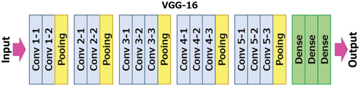
Figure 1: VGG-16 architecture [25]

3.6 DenseNet

DenseNet is a densely related CNN that is built of dense blocks wherein every layer is directly related to each different layer in a feed-ahead way. In this, for every layer the function maps of all preceding layers are dealt with as separate inputs whilst its own feature maps are surpassed on as inputs to all next layers. This creates a deep supervision as each layer receives more supervision. The Fig. 2 represents the architecture of densely connected CNN.

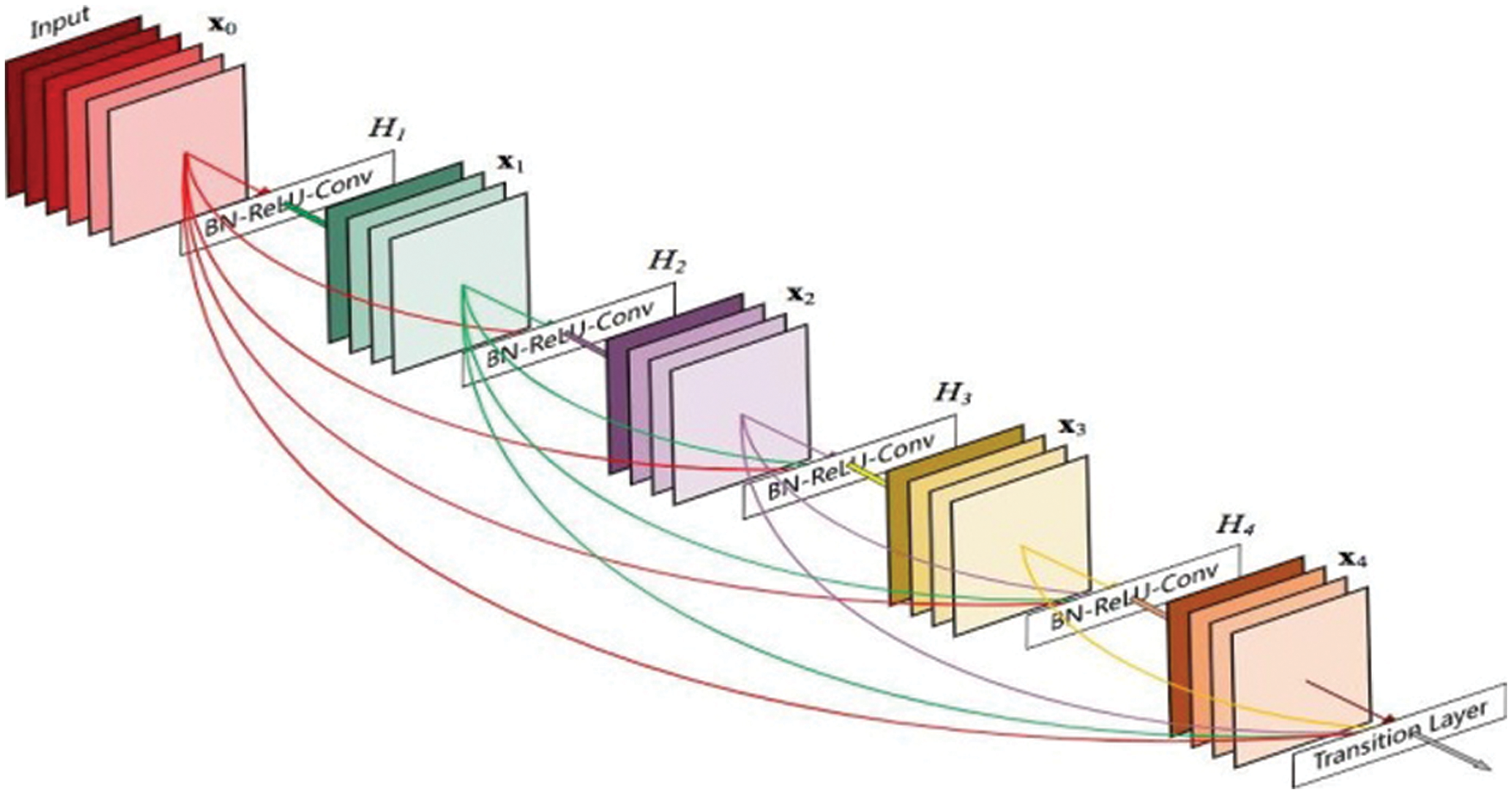
Figure 2: DenseNet architecture [25]

4  Proposed Method

The proposed approach was build and compares various Hybrid models using Transfer Learning with traditional machine learning algorithms. In this work we have used various transfer learning CNN models from the imagenet dataset for feature extraction as given in the Fig. 3. The final extracted data was then trained on fully connected neural networks with a SoftMax classifier. For transfer learning, we’ve used a variety of deep learning architectures (VGG16, VGG19, ResNet50, DenseNet 169, DenseNet201, MobilNet and the EfficientNet). All of these deep learning models were trained on the ImageNet dataset and have attained great accuracy over time. Furthermore, we used the CNN architectures of these models in this work, and then delivered layers based on the dataset’s complexity requirements. The initial set of studies had been completed, and this data augmentation was used to see what changes had occurred.

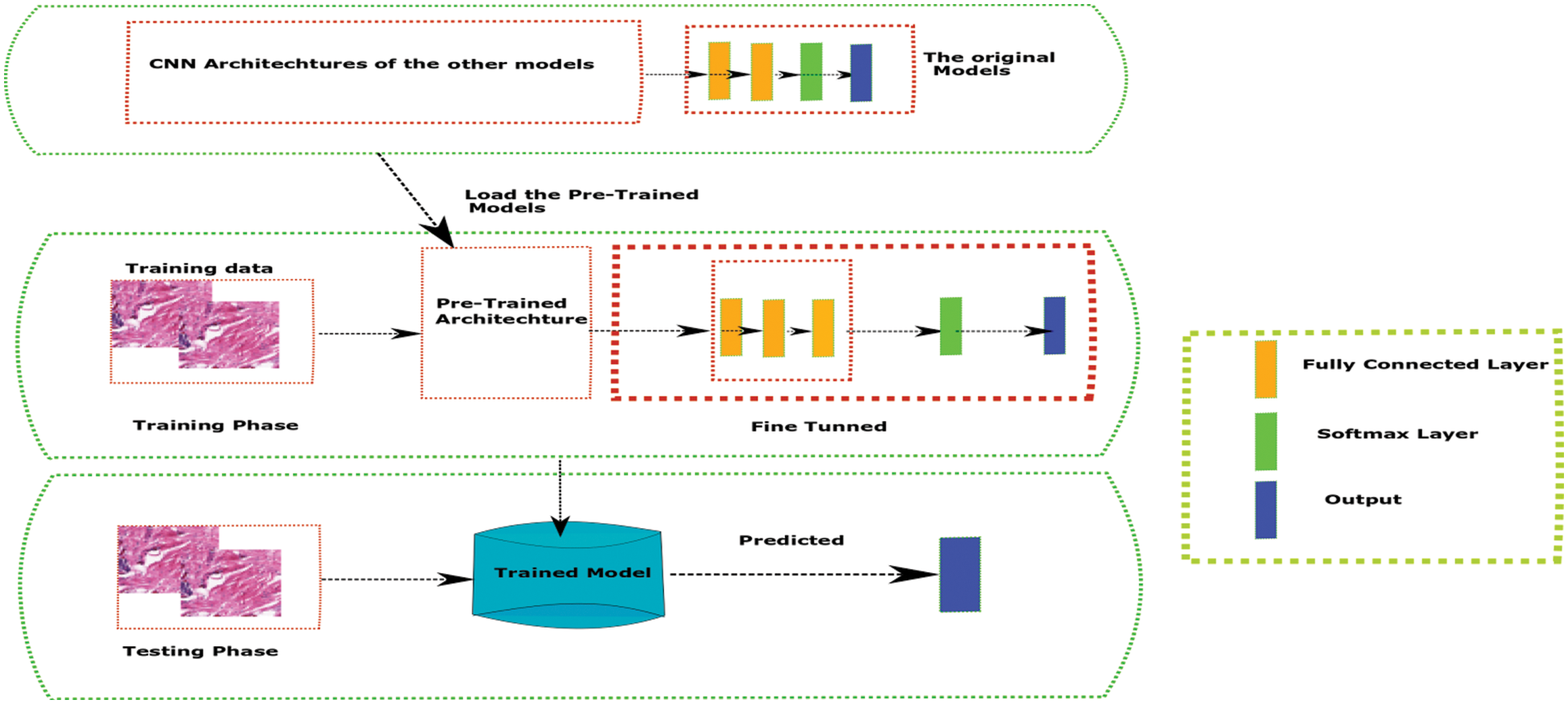
Figure 3: Transfer learning approach with neural networks architecture

4.1 VGG and Logistic Regression

We constructed a hybrid model using VGG and a logistic regression model as shown in Fig. 4. We used the CNN architecture of a pre-trained network VGG with ImageNet weights and passed our whole dataset through it. This step helps in the feature extraction step for our ML algorithms. This acts as our new input for the logistic regression model.

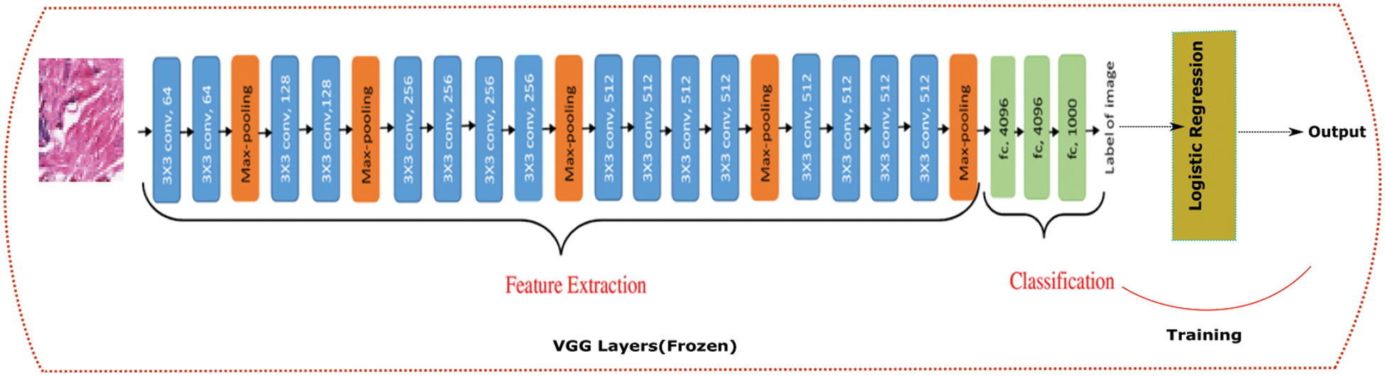
Figure 4: VGG19 + Logistic regression architecture

4.2 VGG and Random Forest

Simonyan and Zisserman introduced the VGG network design in their 2014 research. The simplicity of this network is highlighted by the use of only 33 convolutional layers stacked on top of each other in increasing depth. Max pooling is used to reduce the size of a volume. The Soft-Max classifier is then followed by two fully connected layers, each with 4,096 nodes. The previous architecture was changed a bit and logistic regression was replaced with random forest as shown in Fig. 5.

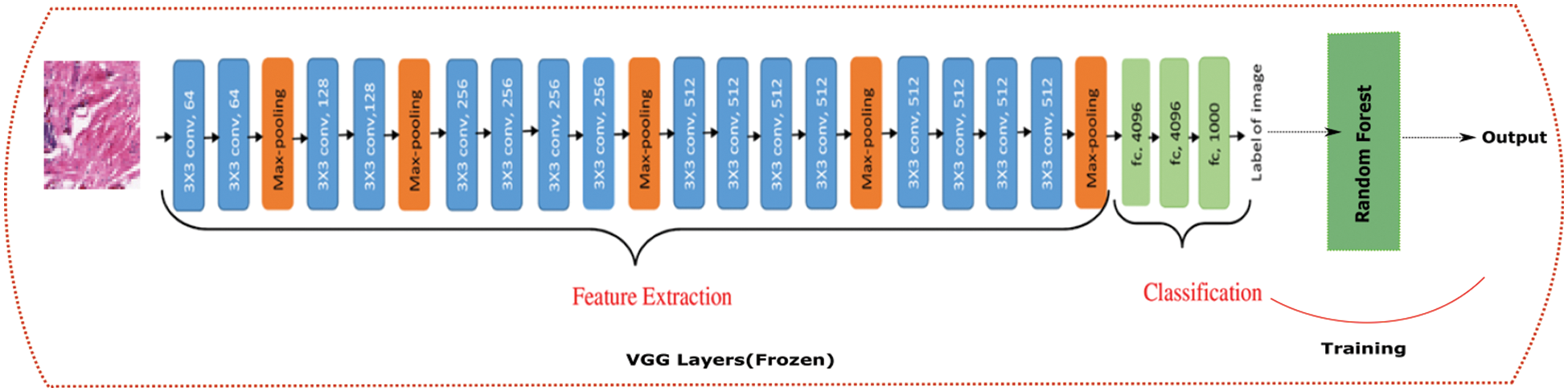
Figure 5: VGG19 + Random forest architecture

4.3 DenseNet with Random Forest

Further, we constructed a different model where we used DenseNet [45] and a random forest model as shown in Fig. 6. We used the CNN architecture of a pre-trained network. DenseNet with ImageNet weights and passed our whole dataset through it. This step helps in the feature extraction step for our ML algorithms. This acts as our new input for the random forest model.

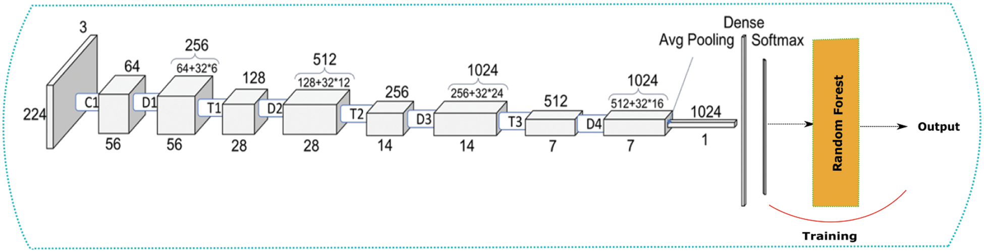
Figure 6: DenseNet + Random forest architecture

4.4 DenseNet with Logistic Regression

The previous architecture was changed a bit and Random Forest was replaced with Logistic Regression as shown in the Fig. 7.

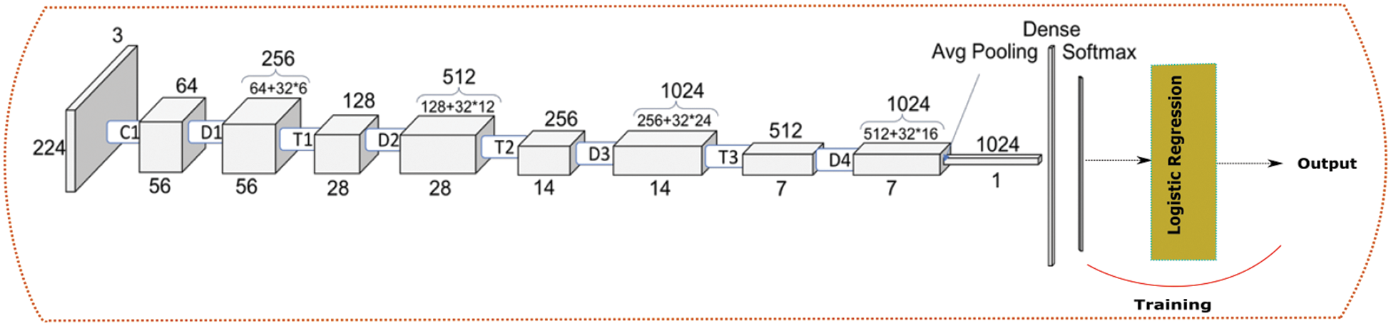
Figure 7: DenseNet + Logistic regression architecture

4.5 Combination of VGG, DenseNet with Logistic Regression

In this model, we combined two ImageNet models. We took VGG and DenseNet CNN layers and passed our data to each of them separately. They both completed their feature extraction step and the output generated were concatenated together before passing it through the ML algorithms. The model we constructed in this step was presented in the Fig. 8.

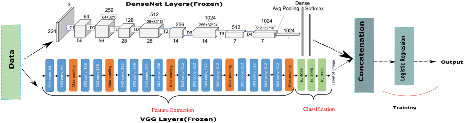
Figure 8: VGG + DenseNet hybrid architecture

5  Experimental Results and Discussion

Several tests examining the performance of the proposed model on the Kaggle dataset are described in this section. The accuracy, precision, sensitivity, septicity, and area under curve (AUC) of various DL models (Inception V3, Inception-V2 ResNet, VGG16, VGG19, and ResNet50) are compared using TL.

5.1 Dataset

The dataset contained 25633 Invasive ductal carcinoma (IDC) positive images and 64634 IDC negative images. Each image was of size 50 × 50 were extracted from the original dataset. Some of the example images can be seen in Fig. 9.

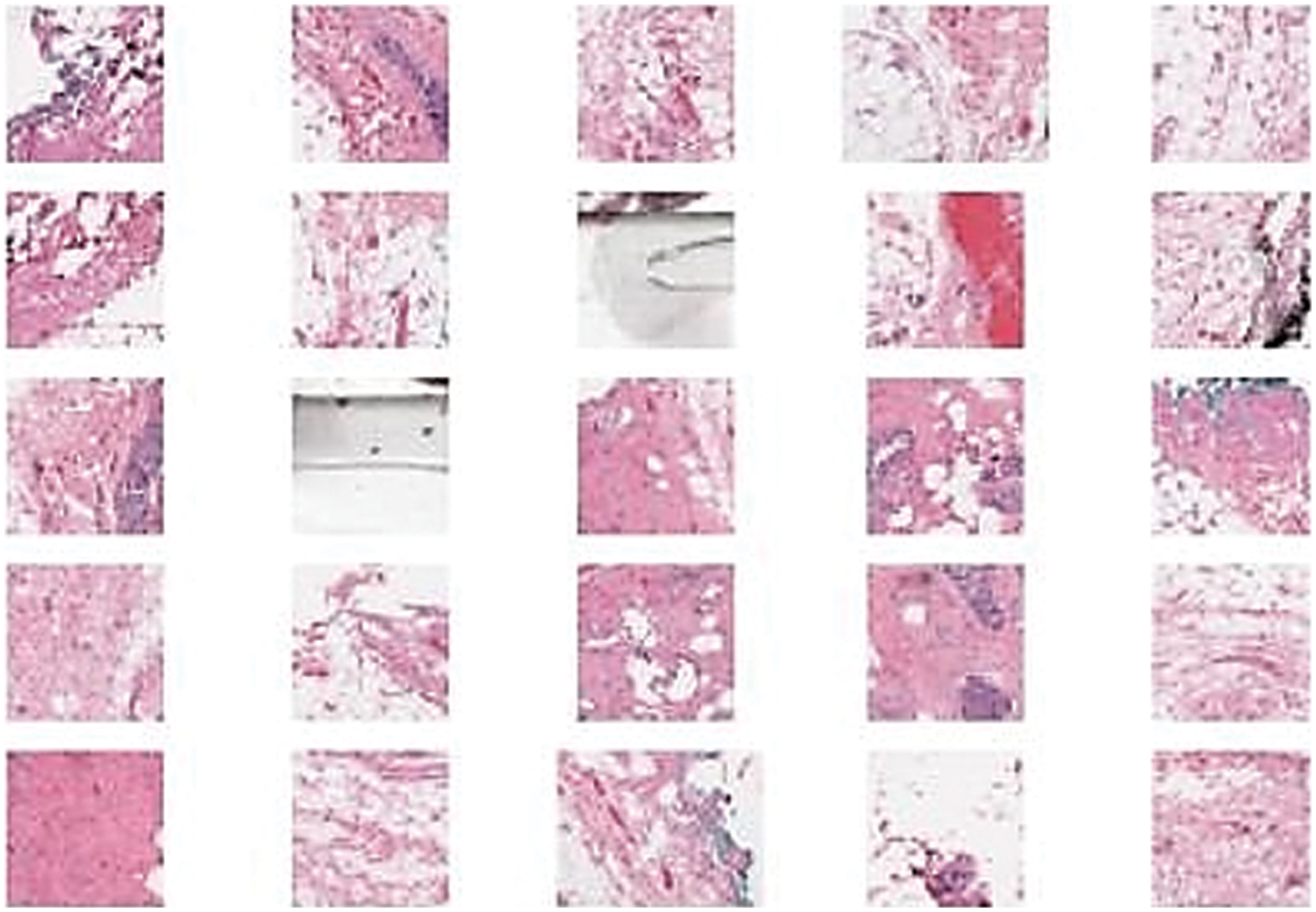
Figure 9: Sample images of breast cancer tissues

5.2 Data Pre-Processing

The dataset was highly imbalanced and thus we performed under-sampling technique to balance the dataset. The under-sampling was done at random to create a target test set. The data contains certain drawbacks which need to be addressed along with it. Therefore, we need to apply some traditional preprocessing techniques and thus we could make our model robust and increase its efficiency.

a:   Normalization: Image Normalization is a typical image processing task that changes the range of pixel intensity values. Range of pixel values goes from 0–255 and in our dataset, the pixel intensity variation is as shown in Fig. 10.

b:    Data Resampling: The dataset we are dealing with is highly imbalanced which is evident in most of the medical domain problems, a negative result is dominant over positive results as shown in the Fig. 11. Therefore, we applied data under sampling techniques to balance both the classes and thus our model does not get biased over any one class. Fig. 12 shows the final class distribution after down and up sampling.

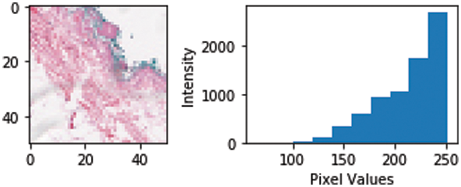
Figure 10: Pixel intensity histogram plot

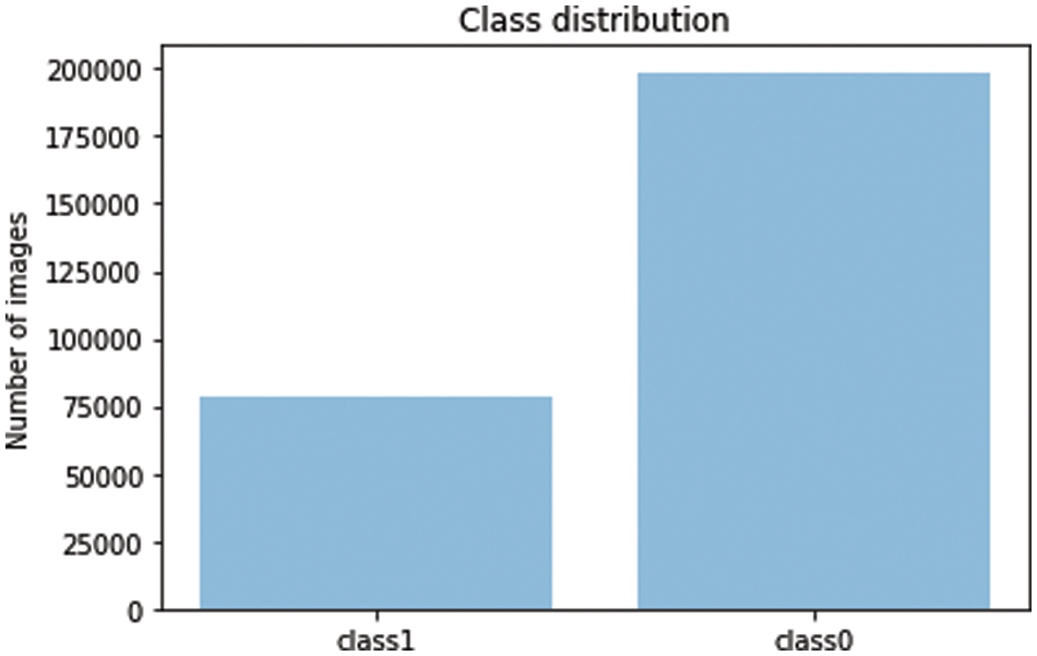
Figure 11: Imbalanced dataset

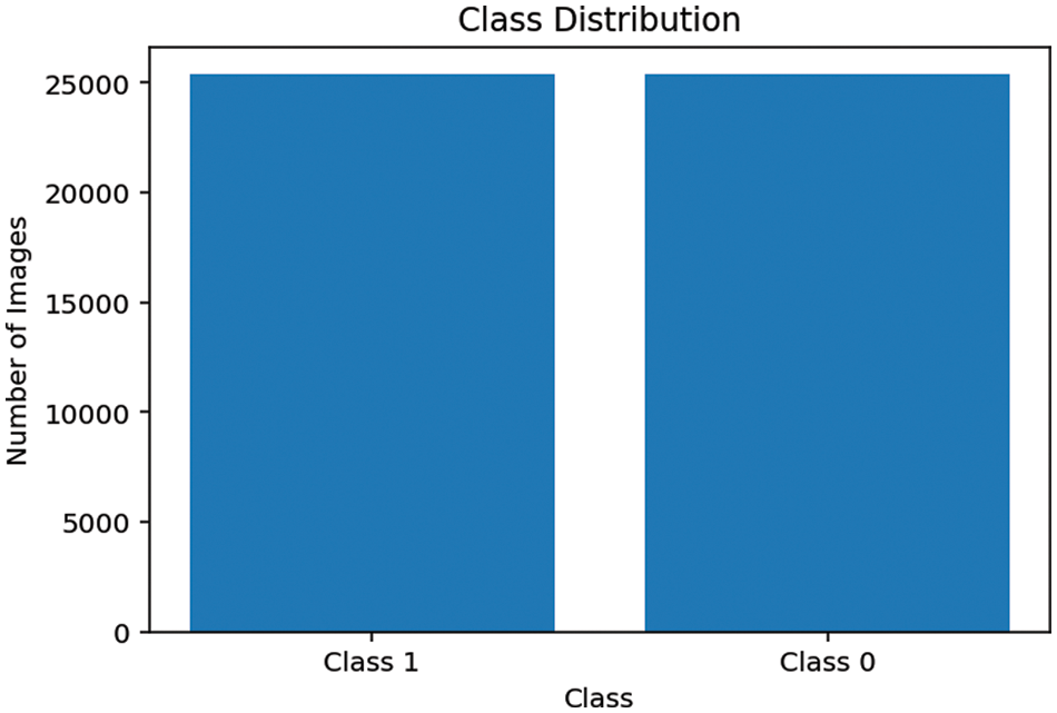
Figure 12: Final class distribution of training set

The final distribution contains 25367 positive samples and 25366 negative samples of training and validation data. Final data split into the train, test and valid sets containing 31393, 7849, 11490 files respectively. The class names were extracted from the names of the files and were one-hot encoded. For example, binary class was represented by two features instead of one, for example, class0 was represented by an array of {1, 0} and class1 was represented by {0, 1} and thus for deep learning model will give probabilities for the two indexes of the array and whichever is maximum that index will be the class of our array.

5.3 Evaluation Indicators

To compare the performance of various DL architectures, most common evaluation indicators are classification accuracy, sensitivity, specificity, Area under Curve (AUC) and confusion matrix. Tab. 1 shows comparison between predicted and actual labels. From this table, we can evaluate other evaluation indicators.

Classification Accuracy: This indicator tells us about correct predictions made by our trained model on unseen new images from the test set. The mathematical formula of classification accuracy is as given in Eq. (1)

Classification Accuracy=No.of correct prediction on test set size of test set=(TP+TN)(TP+TN)+FP+FN(1)

True Positive (TP): Sample that is correctly classified as positive same as ground truth.

False Positive (FP): Samples that is wrongly classified as positive as opposed to ground truth.

True negative (TN): Sample that is correctly classified as negative same as ground truth.

False negative (FN): Samples that is wrongly classified as negative as opposed to ground truth.

Sensitivity: It is the proportion of positive samples that were classified as positive. Higher sensitivity indicates that the system can accurately predict the presence of disease and false negative cases will be very less. It is mathematically defined as in Eq. (2).

sensitivity=TPTP+FN (2)

Specificity: It shows the proportion of negative samples that were classified as negative. Higher specificity means that the system is making correct predictions about healthy people. It is defined as in Eq. (3).

specificity=TNTN+FP(3)

Precision and Recall are defined as in Eq. (4).

Precsion=TPTP+FP,Recall=TPTP+FN(4)

F-Score is harmonic mean Precision (P) and Recall (R). It is defined as in Eq. (5).

F−score=2 ∗ P ∗ R(P+R)(5)

The Receiver Operator Characteristic (ROC) curve is graph between sensitivity and (1-specificity). It is used to analyses the trade-off between sensitivity and specificity.

Area under Curve (AUC): Higher AUC means that the model can better distinguish between positive and negative classes.

Confusion Matrix: It is a table that shows predictions made by the model in terms of TP, TN, FP and FN as shown in the Tab. 1

Performance Evaluation: Finally the trained model from the proposed architecture is tested against test-set and various performance metrics like accuracy, sensitivity, specificity, F-score, AUC are computed. The confusion matrix was also evaluated for the model [46–50].

We experimented with our proposed hybrid models on Kaggle dataset for three split ratios, 20%, 30% and 40%. Although this dataset was imbalanced, we overcame this problem by under sampling [51–53].

5.4 Experimental Results

Our approach in this work includes, implementing various hybrid models and comparing and evaluating them. The experiment was conducted by applying transfer learning with traditional ML algorithms. Therefore, we implemented five models namely VGG + (Logistic Regression/Random Forest), DenseNet + (Random Forest/Logistic Regression) and a super hybrid model which was implemented by concatenating the results of VGG and DenseNet and applying Logistic Regression in final layers.

5.5 Transfer Learning with Traditional Machine Learning Algorithm

Various architectures were used as transfer learning models. Their weights were trained on an ImageNet dataset and input shape was changed to (50, 50, 3) (the size of the image of our dataset). We imported only the CNN architectures of the models and excluded the fully connected layers. The output of imported CNN layers was converted into 1D vector and then used as a training input for our traditional ML algorithms. The data supplied to CNN were augmented with the following specification as shown in Tab. 2.

Moreover, we have performed the various hyper parameter tuning to get the best result. The performance of hybrid models is represented through F-score shown in Tab. 3. Traditional ML algorithms used with transfer learning models (best ones) with their F-Score and AUC value is shown in Tab. 4.

Another experiment was done using a hybrid of VGG and DenseNet. The image augmented data was passed through VGG and through DenseNet. The output of both the architectures were concatenated and then passed as training input for the logistic regression model and the result for the AUC and the F-Score is shown in the Tab. 5.

5.6 Transfer Learning Model with Custom Made Fully Connected Layers

The experiments were performed on Kaggle Notebook with its GPU with Keras API of TensorFlow. NVidia K80 GPU was used to perform experiments on the dataset. We used various famous DL architectures for transfer learning (VGG16, VGG19, ResNet50, DenseNet169, DenseNet121, DenseNet201, MobileNet and EfficientNet). All these models were trained on the ImageNet dataset and over the years they have achieved high accuracy of the dataset. We have used only CNN architectures of these models and then added layers according to the requirement of the complexity of the dataset. The first sets of experiments were conducted. Without any data augmentation and then data argumentation was added to see the change. The evaluation metrics used to compare results were f1-score, recall, precision, accuracy, specificity and sensitivity. They are used to evaluate our model using true positives, true negatives, false positives and false negatives.

DenseNet169 was trained for 60 epochs with a global pooling layer and two dense layers each followed by a dropout layer of 0.15 and 0.25 respectively with ReLU activation added after the frozen CNN layers. The last layer was a dense layer with two classes and a SoftMax function. DenseNet 121, ResNet50, VGG19 and VGG16 were trained for 60, 60, 100, 100 epochs respectively. The architecture of the last layers was made different from DenseNet169. We added batch normalization having 1e-05 epsilon value and 0.1momentum followed by a dense layer with 512 nodes and a dropout of 0.45. After that, a dense layer with 2 nodes representing each class was added with SoftMax activation. The experiment results without data augmentation and with data augmentation can be seen in Tabs. 6 and 7 respectably and the highest value in each column is highlighted. Also the Confusion matrix of DenseNet 169 with data augmentation is presented in the Fig. 13.

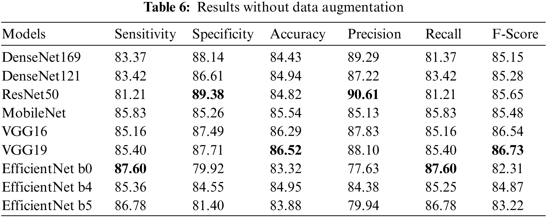
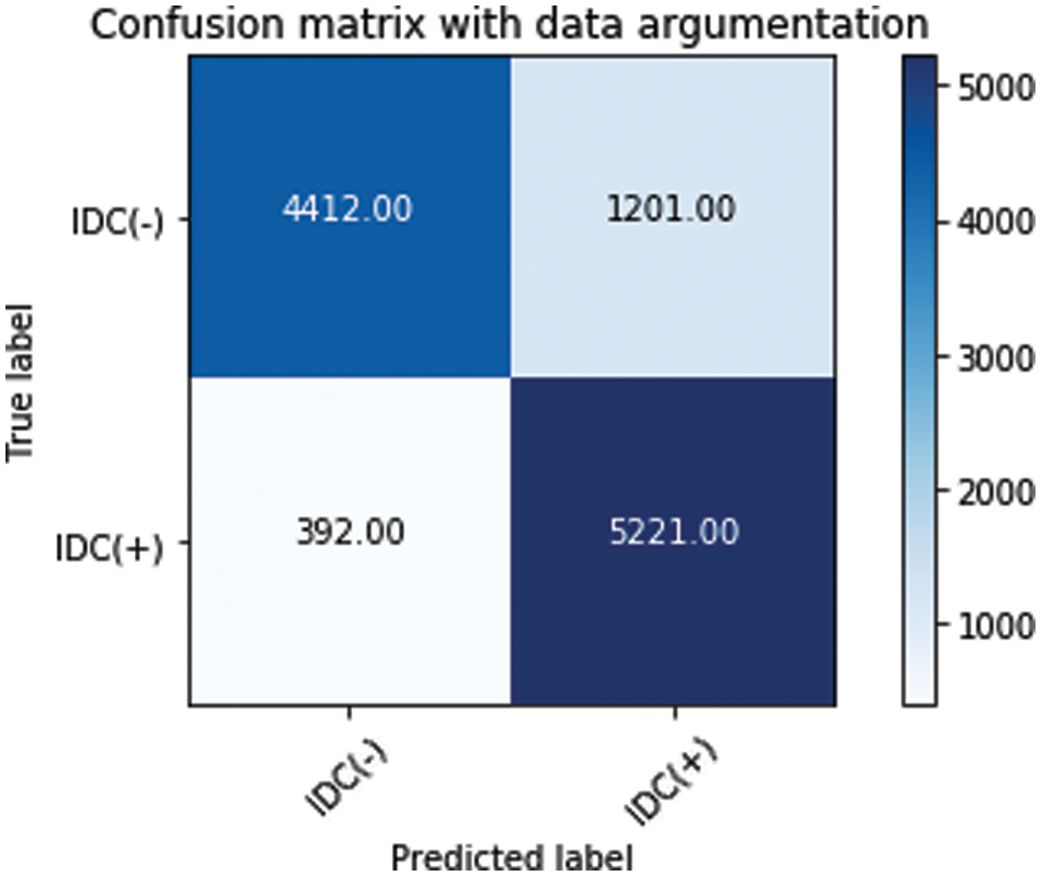
Figure 13: Confusion matrix of DenseNet 169 with data augmentation

Tab. 8 compares our best model’s efficiency with respect to the efficiency claimed by previous works. For more clarity of the work. Figs. 14a–14d depicts the area under the curve (AUC) of the various models and Figs. 15a–15e presents the confusion matrix. Fig. 16 presents the comparison of transfer learning and traditional ML algorithms of different approaches as well as the hybrid model.

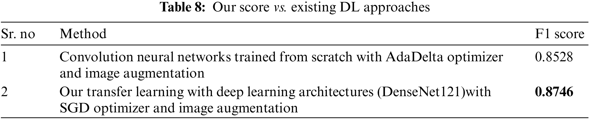
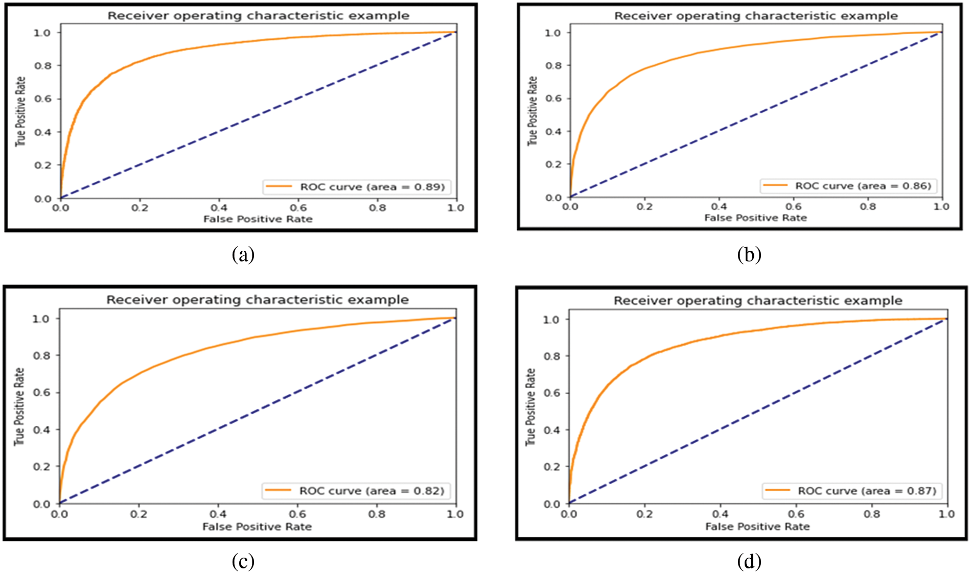
Figure 14: (a) AUC curve of VGG + Logistic regression model, (b) AUC curve of DenseNet + Random forest model, (c) AUC curve of DenseNet with logistic regression model, (d) AUC curve of VGG + Random forest model

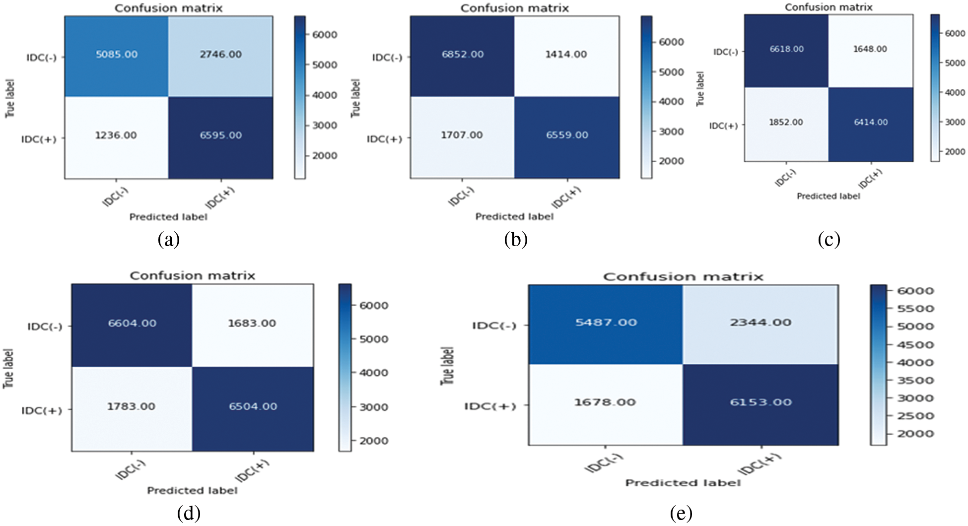
Figure 15: (a) Confusion matrix of VGG and logistic regression, (b) Confusion matrix of DenseNet and logistic, (c) Confusion matrix of DenseNet and random forest, (d) Confusion matrix of VGG and random forest, (e) Confusion matrix of VGG + Dense and logistic regression

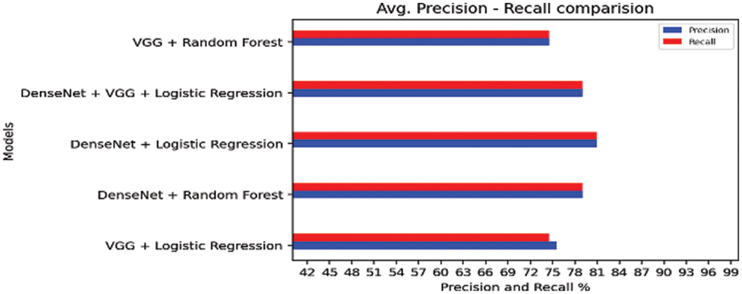
Figure 16: Comparison of transfer learning and traditional machine learning algorithms

The receiver operating characteristic curve (ROC curve) is a performance metric for classifying problems at various threshold settings. The area under the curve (AUC) represents the degree or measure of sap arability. It indicates the degree to which the model is capable of discriminating between classes.

The larger the AUC, the more accurately the model predicts 0 class as 0 and 1 class as 1.When VGG model is coupled with logistic regression, the combined architecture delivered AUC of 0.89 which is highest of other three combinations coupling of DenseNet with Random Forest Model, DenseNet with Logistic Regression Model, VGG combined with Random Forest Model. That indicate that the hybrid of VGG and logistic regression can better distinguish better malignant class and benign class than the other hybrid combinations. The AUC value for all hybrid models are comparable and all of the hyrid models can well distinguish between the two classes.

From the Tab. 9 below, we find that average false rate of hybrid models VGG with Logistic. DenseNet with Random forest, DenseNet with Logistic regression, VGG with Random forest, and VGG, DenseNet and logistic are 0.25, 0.18, 0.21, 0.20 and 0.26 respectively. Out of these hybrid models we find that misclassification rate is minimum when DenseNet is coupled with logistic regression.

6  Conclusion

Breast cancer classification using multiple methods such as cross-validation, pipelining, model selection and the different ML hybrid classification models have played a great role We took advantage of various pre-trained models and used their knowledge and added some fine-tuning to get an efficient model. We first tried under sampling techniques to balance classes then image argumentation followed by transfer learning. We were able to get a high precision and moderate recall model with VGG19 with image argumentation. We have obtained that maximum result is shown by DenseNet + logistic regression showing the F-score of 0.81 for both classes. Furthermore, using different classification we have obtained VGG + logistic regression (F-score: 0.73), VGG + random forest (F-score: 0.74), DenseNet + random forest (F- score: 0.79) and hybrid of VGG + Densenet + logistic regression (F-score: 0.79). Moreover, the results and classification can be optimized with the help of GAN’.As the used dataset contained more negative samples than the positive samples, GAN’s would help to create more samples and thus more training data set to be trained and learned from. However, using GANs in medical images cannot assure true labelled data. This indeed is a limitation for medical image data. Hence we can conclude that transfer learning which the simplest technique available in DL frameworks can be used to detect dangerous diseases such as cancer. Thus, in the future, we are planning to work on the full dataset with full-size slide images and will work with more advanced techniques such as GAN networks to obtain better results.

Acknowledgement: This research work was partially supported by JSS Academy of Technical Education, Prince Sattam Bin Abdulaziz University and Chiang Mai University.

Funding Statement: The authors received no specific funding for this study.

Conflicts of Interest: The authors declare that they have no conflicts of interest to report regarding the present study.

References

1. E. Myers, “Benefits and harms of breast cancer screening,” JAMA, vol. 314, no. 15, pp. 1615–1632, 2015. [Google Scholar]
2. L. Havrilesky, J. Gierisch, P. Moorman, D. McCrory, S. Ghateet et al., “Systematic review of cancer screening literature for updating American cancer society breast cancer screening guidelines,” Duke Evidence Synthesis Group for American Cancer Society, vol. 179, no. 1, pp. 220–245, 2014. [Google Scholar]
3. S. Singh and B. K. Tripathi, “Pneumonia classification using quaternion deep learning,” Multimedia Tools and Application, vol. 81, no. 2, pp. 1743–1764, 2022. [Google Scholar]
4. M. H. Motlagh, M. Jannesari, H. Aboulkheyr, P. Khosravi, O. Elemento et al., “Breast cancer histopathological image classification: A deep learning approach,” in 2018 IEEE Int. Conf. on Bioinformatics and Biomedicine (BIBM), Madrid, Spain, pp. 242881–242899, 2018. [Google Scholar]
5. B. Bejnordi, G. Zuidhof, M. Balkenhol, P. Bult, B. Vanginneken et al., “Context-aware stacked convolutional neural networks for classification of breast carcinomas in whole-slide histopathology images,” Journal of Medical Imaging, vol. 4, no. 4, pp. 1–28, 2017. [Google Scholar]
6. A. Rakhlin, A. Shvets, V. Iglovikov and A. Kalinin, “Deep convolutional neural networks for breast cancer histology image analysis,” in Int. Conf. on Image Analysis and Recognition, Póvoa de Varzim, Portugal, pp. 737–744, 2018. [Google Scholar]
7. K. Nisar, Z. Sabir, M. A. Z. Raja, A. A. A. Ibrahim, J. J. Rodrigues et al., “Artificial neural networks to solve the singular model with neumann–robin, dirichlet and neumann boundary conditions,” Sensors, vol. 21, no. 19, pp. 6498–6520, 2021. [Google Scholar]
8. S. Rawat, S. Alghamdi, G. Kumar, Y. Alotaibi, O. Khalaf et al., “Infrared small target detection based on partial Sum minimization and total variation,” Mathematics, vol. 10, no. 4, pp. 671–680, 2022. [Google Scholar]
9. L. Wang, L. Zhang and Z. Yi, “Trajectory predictor by using recurrent neural networks in visual tracking,” IEEE Transactions on Cybernetics, vol. 47, no. 10, pp. 3172–3183, 2017. [Google Scholar]
10. Y. Wang, L. Zhang, L. Wang and Z. Wang, “Multi-task learning for object localization with deep reinforcement learning,” IEEE Transactions on Cognitive and Developmental Systems, vol. 11, no. 4, pp. 573–580, 2019. [Google Scholar]
11. J. Hu, Y. Chen, J. Zhong, R. Ju and Z. Yi, “Automated analysis for retinopathy of prematurity by deep neural networks,” IEEE Transactions on Medical Imaging, vol. 38, no. 1, pp. 269–279, 2019. [Google Scholar]
12. J. Mo, L. Zhang and Y. Feng, “Exudate-based diabetic macular edema recognition in retinal images using cascaded deep residual networks,” Neurocomputing, vol. 290, no. 3, pp. 161–171, 2018. [Google Scholar]
13. X. Qi, L. Zhang, Y. Chen, Y. Pi, Y. Chen et al., “Automated diagnosis of breast ultrasonography images using deep neural networks,” Medical Image Analysis, vol. 52, no. 2, pp. 185–198, 2019. [Google Scholar]
14. Q. Zhang, L. T. Yang, Z. Chen and P. Li, “A survey on deep learning for big data,” Information Fusion, vol. 42, no. 1, pp. 146–157, 2018. [Google Scholar]
15. Z. Cai, J. Gu, J. Luo, Q. Zhang, H. Chen et al., “Evolving an optimal kernel extreme learning machine by using an enhanced grey wolf optimization strategy,” Expert System with Applications, vol. 138, no. 3, pp. 3412–3429, 2019. [Google Scholar]
16. C. Yan, X. Chang, M. Luo, Q. Zheng, X. Zhang et al., “Self-weighted robust LDA for multiclass classification with edge classes,” ACM Transaction on Intelligent System Technology, vol. 12, no. 1, pp. 1–19, 2020. [Google Scholar]
17. X. Zhang, M. Fan, D. Wang, P. Zhou and D. Tao, “Top-k feature selection framework using robust 0–1 integer programming,” IEEE Transaction on Neural Network Learning System, vol. 32, no. 7, pp. 3005–3018, 2021. [Google Scholar]
18. X. Zhang, T. Wang, J. Wang, G. Tang and L. Zhao, “Pyramid channel based feature attention network for image dehazing,” Computer Vision and Image Understanding, vol. 198, no. 2, pp. 3657–3673, 2020. [Google Scholar]
19. X. Zhang, R. Jiang, T. Wang, P. Huang and L. Zhao, “Attention-based interpolation network for video deblurring,” Neurocomputing, vol. 453, no. 2, pp. 865–875, 2020. [Google Scholar]
20. W. Liu, X. Chang, L. Chen, D. Phung, X. Zhang et al., “Pair-based uncertainty and diversity promoting earlyactive learning for person reidentication,” ACM Transaction on Intelligent System Technology, vol. 11, no. 2, pp. 1–15, 2020. [Google Scholar]
21. X. Zhang, T. Wang, W. Luo and P. Huang, “Multi-level fusion and attention-guided CNN for image dehazing,” IEEE Transaction on Circuits System and Video Technology, vol. 57, no. 2, pp. 5673–5691, 2020. [Google Scholar]
22. K. Weiss, “Survey of transfer learning,” Journal of Big Data, vol. 3, no. 1, pp. 1–40, 2016. [Google Scholar]
23. X. Y. Mingyuan and Y. Wang, “Research on image classification model based on deep convolution neural network,” EURASIP J Image & VideoProcess, vol. 1, no. 2, pp. 1–11, 2019. [Google Scholar]
24. A. Krizhevsky, I. Sutskever and G. Hinton, “ImageNet classification with deep convolutional neural networks,” ACM Communication, vol. 60, no. 6, pp. 84–90, 2017. [Google Scholar]
25. W. Sun, G. C. Zhang, X. R. Zhang, X. Zhang and N. N. Ge, “Fine-grained vehicle type classification using lightweight convolutional neural network with feature optimization and joint learning strategy,” Multimedia Tools and Applications, vol. 80, no. 20, pp. 30803–30816, 2021. [Google Scholar]
26. S. Rawat, S. K. Verma and Y. Kumar, “Reweighted infrared patch image model for small target detection based on non-convex
27. M. Lazaro, F. Herrera and A. R. F. Vidal, “Ensembles of cost-diverse Bayesian neural learners for imbalanced binary classification,” Information Sciences, vol. 520, no. 3, pp. 31–45, 2020. [Google Scholar]
28. Y. Shao, W. Chen, J. Zhang, Z. Wang and N. Y. Deng, “An efficient weighted lagrangian twin support vector machine for imbalanced data classification,” Pattern Recognition, vol. 47, no. 9, pp. 3158–3167, 2014. [Google Scholar]
29. B. Krawczyk, M. Wozniak and G. Schaefer, “Cost-sensitive decision tree ensembles for effective imbalanced classification,” Applied Soft Computing, vol. 14, no. 1, pp. 554–562, 2014. [Google Scholar]
30. Z. Q. Zhao, “A novel modular neural network for imbalanced classification problems,” Pattern Recognition Letters, vol. 30, no. 9, pp. 783–788, 2009. [Google Scholar]
31. Q. Zou, S. Xie, Z. Lin, M. Wu and Y. Ju, “Finding the best classification threshold in imbalanced classification,” Big Data Research, vol. 5, no. 1, pp. 2–8, 2016. [Google Scholar]
32. Y. Li, J. Huang, N. Ahuja and M. Yang, “Joint image filtering with deep convolutional networks,” IEEE Transactions on Pattern Analysis and Machine Intelligence, vol. 41, no. 8, pp. 1909–1923, 2019. [Google Scholar]
33. N. Wahab and A. Khan, “Multifaceted fused-CNN based scoring of breast cancer whole-slide histopathology images,” Applied Soft Computing, vol. 97, no. 2, pp. 106808–106832, 2020. [Google Scholar]
34. G. Murtaza, L. Shuib and A. Abdul, “Deep learning-based breast cancer classification through medical imaging modalities: State of the art and research challenges,” Artificial Intelligence Review, vol. 53, no. 3, pp. 1655–1720, 2020. [Google Scholar]
35. S. Z. Ramadan, “Using convolutional neural network with cheat sheet and data augmentation to detect breast cancer in mammograms,” Computational and Mathematical Methods in Medicine, vol. 2020, Article ID 9523404, pp. 1–9, 2020. [Google Scholar]
36. M. Masud, A. E. Rashed and M. S. Hossain, “Convolutional neural network-based models for diagnosis of breast cancer,” Neural Computing and Applications, vol. 5, no. 2, pp. 345–358, 2020. [Google Scholar]
37. L. Tsochatzidis, P. Koutla, L. Costaridou and I. Pratikakis, “Integrating segmentation information into CNN for breast cancer diagnosis of mammographic masses,” Computer Methods and Programs in Biomedicine, vol. 200, no. 2, pp. 105913–105935, 2021. [Google Scholar]
38. F. Pérez, F. Signol, J. P. Cortes, A. Fuster, M. Pollan et al., “A deep learning system to obtain the optimal parameters for a threshold-based breast and dense tissue segmentation,” Computer Methods and Programs in Biomedicine, vol. 195, no. 2, pp. 105668–105682, 2020. [Google Scholar]
39. G. Murtaza, L. Shuib, A. Wahab, G. Mujtaba, H. Nwekeet et al., “Deep learningbased breast cancer classification through medical imaging modalities: State of the art and research challenges,” Artificial Intelligence Review, vol. 53, no. 3, pp. 1655–1720, 2020. [Google Scholar]
40. S. Pan and Q. Yang, “A survey on transfer learning,” IEEE Transactions on Knowledge and Data Engineering, vol. 22, no. 10, pp. 1345–1359, 2009. [Google Scholar]
41. X. R. Zhang, J. Zhou, W. Sun, S. K. Jha, “A lightweight CNN based on transfer learning for COVID-19 diagnosis,” Computers, Materials & Continua, vol. 72, no. 1, pp. 1123–1137, 2022. [Google Scholar]
42. S. Rawat, S. K. Verma and Y. Kumar, “Infrared small target detection based on non-convex triple tensor factorization,” IET Image Processing, vol. 15, no. 2, pp. 556–570, 2021. [Google Scholar]
43. B. Kamiński, M. Jakubczyk and P. Szufel, “A framework for sensitivity analysis of decision trees,” Central European Journal of Operations Research, vol. 26, no. 1, pp. 135–159, 2017. [Google Scholar]
44. K. Tin, “The random subspace method for constructing decision forests,” IEEE Transactions on Pattern Analysis and Machine Intelligence, vol. 20, no. 8, pp. 832–844, 1998. [Google Scholar]
45. G. Huang, Z. Liu, L. Van, D. Maatenand and K. Weinberger, “Densely connected convolutional networks,” in IEEE Conf. on Computer Vision and Pattern Recognition, Honolulu, USA, pp. 4700–4708, 2017. [Google Scholar]
46. C. Drummond and R. C. Holte, “C4.5, class imbalance, and cost sensitivity: Why under-sampling beats over-sampling,” Workshop on Work and Learn from Imbalanced Datasets II, ICML, Washington DC, pp. 345–358, 2003. [Google Scholar]
47. M. Umar, Z. Sabir, M. A. Z. Raja, M. Gupta, D. N. Le et al., “Computational intelligent paradigms to solve the nonlinear SIR system for spreading infection and treatment using Levenberg–Marquardt backpropagation,” Symmetry, vol. 13, no. 4, pp. 618–636, 2021. [Google Scholar]
48. M. Gupta, J. Lechner and B. Agarwal, “Performance analysis of Kalman filter in computed tomography thorax for image denoising,” Recent Advances in Computer Science and Communications, vol. 13, no. 6, pp. 1199–1212, 2020. [Google Scholar]
49. M. Gupta, H. Taneja, L. Chand and V. Goyal, “Enhancement and analysis in MRI image denoising for different filtering techniques,” Journal of Statistics and Management Systems, vol. 21, no. 4, pp. 561–568, 2018. [Google Scholar]
50. K. Nisar, Z. Sabir, M. A. Z. Raja, A. A. A. Ibrahim, J. J. Rodrigues et al., “Evolutionary integrated Heuristic with Gudermannian neural networks for second kind of Lane–Emden nonlinear singular models,” Applied Sciences, vol. 11, no. 11, pp. 4725–4740, 2021. [Google Scholar]
51. M. Gupta, H. Taneja and L. Chand, “Performance enhancement and analysis of filters in ultrasound image denoising,” Procedia Computer Science, vol. 132, no. 1, pp. 643–652, 2018. [Google Scholar]
52. A. Kumar, S. Chakravarty, M. Gupta, I. Baig and M. A. Albreem, “Implementation of mathematical morphology technique in binary and grayscale image,” in Advance Concepts of Image Processing and Pattern Recognition, 1st ed., USA: Springer, pp. 203–212, 2022. [Google Scholar]
53. S. Kumar, P. Kumar, M. Gupta and A. K. Nagawat, “Performance comparison of median and wiener filter in image de-noising,” International Journal of Computer Applications, vol. 12, no. 4, pp. 27–31, 2010. [Google Scholar]
Cite This Article
Copyright © 2023 The Author(s). Published by Tech Science Press.
This work is licensed under a Creative Commons Attribution 4.0 International License , which permits unrestricted use, distribution, and reproduction in any medium, provided the original work is properly cited.
Downloads
Citation Tools