Data Mining with Comprehensive Oppositional Based Learning for Rainfall Prediction

1  Introduction

Data mining (DM) is the process of examining massive dataset for the identification of patterns and relationships which helps to resolve business problem by data analysis [1]. DM tools and technologies can be used for predicting future trends and decision making [2]. It is commonly employed by business intelligence and data analytics teams, assisting them to extract knowledge for huge quantity of data. It aims to extract and discover patterns in large sized data with the inclusion of machine learning, statistics, and database systems [3]. It finds useful in several applications in different areas such as education, healthcare, environmental monitoring, finance, banking industry, etc [4,5]. On the other hand, rainfall prediction has existed for a long time with conventional models that utilize statistical approaches [6,7] for assessing the relationships among the rainfall, geographic coordinate includes latitude and longitude, and atmospheric factor includes temperature, pressure, humidity, and wind speed. But, the difficulty of rainfall namely non-linearity makes them hard to forecast.

Statistical and mathematical approaches could be time-consuming with minor consequences and employ complex computational power. Machine learning (ML) based approach employs self-learning capacity to attain hidden features of echo variations and displays association and good memory capability [8]. It is employed as numerical prediction and classification model in climate prediction shows the broad and potential predictions of employing neural network systems to radar echo extrapolation [9]. Especially, it has lately employed deep learning (DL) method for processing meteorological big data, shows stronger technical performance and advantages, that has gained considerable interest from the research [10].

This article develops a novel comprehensive oppositional moth flame optimization with deep learning enabled rainfall prediction (COMFO-DLRP) technique for environmental monitoring. The proposed CMFO-DLRP model undergoes data pre-processing and correlation matrix (CM) based feature selection processes. Besides, deep belief network (DBN) model is applied for the effective prediction of rainfall data. Furthermore, COMFO technique was derived by integrating the concepts of comprehensive oppositional based learning (COBL) with traditional MFO algorithm. At last, the COMFO algorithm is employed for the optimal hyperparameter selection of the DBN model. For inspecting the improved performance of the COMFO-DLRP approach, a comprehensive experimental analysis was performed and the outcomes are assessed under various measures.

The rest of the paper is organized as follows. Section 2 briefs the existing works, Section 3 discusses the proposed model, Section 4 offers experimental validation, and Section 5 draws conclusion.

2  Literature Review

Sun et al. [11] presented the convolution 3D-gated recurrent unit (GRU), named Conv3D-GRU technique for predicting the future rainfall intensities on a comparatively short interval of time in the ML viewpoint. Primarily, the spatial feature of radar echo map with distinct height was removed by 3D convolutional, next, the radar echo map on time series were coding and decoding with utilize GRU. At last, the training method was utilized for predicting the radar echo map from the next 1–2 h. In [12], different methods and techniques are executed for predicting the rainfall data. The comparison analysis is demonstrated concentrating on evolving and relating various ML techniques, estimating various conditions and time horizons, and predicting rainfall utilizing two kinds of techniques.

Endalie et al. [13] implemented a rainfall prediction method to Jimma, an area placed from south-western Oromia, Ethiopia. It has presented the long short term memory (LSTM) based forecast technique able of predicting Jimma’s daily rainfalls. An experiment is demonstrated for evaluating the presented technique utilizing different metrics. Venkatesh et al. [14] established a rainfall forecast method utilizing generative adversarial network (GAN) for analyzing rainfall data of India and forecasting the future rainfall. The presented technique utilized a GAN network in that LSTM network technique was utilized as generator and convolutional neural network (CNN) technique was utilized as discriminator. In [15], rainfall forecast was implemented for anticipating the damage to embankment. The rainfall forecast is executed utilizing LSTM dependent upon rainfall parameters: El-Nino and Indian Ocean Dipole (IOD). The experimentally are implemented with 2 methods: a primary technique utilized IOD and El-Nino parameters, but the secondary method utilized rainfall time series patterns.

Zhang et al. [16] presented the dual-input dual-encoder recurrent neural network (RNN) such as Rainfall Nowcasting Network (RN-Net), for solving this issue. It gets the past grid rainfall data included by automatic weather station and doppler radar mosaic data as input data after that predicts the grid rainfall data to the next 2h. It can be conducted experiments on the South-eastern China data set. Amine Ben Rhaiem et al. [17] utilized the everyday open rainfall data in the national observatory of Tunisian agriculture (ONAGRI) for developing an ETL (Extract, Transform, and Load) tools for automatically spatializing and loading the old information as to big data platforms with always increment a novel daily disseminated record. Besides, this work implements the Voronoi spatial analysis technique for estimating rainfall measures to the recently more spatial unit in OSM world mapping scheme. Next, according to these spatial estimations, the work studies the possibility of executing ARIMA to time series predicting.

3  The Proposed Model

In this study, a new COMFO-DLRP technique has been developed to predict rainfall and thereby determine the environmental changes. The presented COMFO-DLRP technique encompasses a series of processes namely data pre-processing, CM based feature selection, DBN based prediction, and COMFO based hyperparameter tuning. The COMFO algorithm is designed by incorporating the concepts of COBL with MFO algorithm. Fig. 1 illustrates the process flow of COMFO-DLRP technique.

Figure 1: Process flow of COMFO-DLRP technique

3.1 Data Pre-processing and Feature Selection

Data pre-processing is an essential step in the rainfall prediction model, which transforms the raw data into useful format. Generally, pre-processing involves removal of categorical values, missing values, and structuring one hour of data into a vector row [18]. Besides, the weather condition codes understand weather id, weather description, weather main, and weather icon sub features, which comprises distinct records based on the weather type acquired in one hour. Besides, important features representing the variability of the input data are chosen by the use of CM. It eradicates the existence of repetitive features with no use of target features. Here, Pearson correlation coefficient is utilized for determining CM.

3.2 Design of DBN Based Predictive Model

During prediction process, the DBN model receives the preprocessed data as input to forecast the rainfall precisely. DBN is a basic DNN technique that contains distinct layers such as restricted Boltzmann machine (RBM) and multilayer perceptron (MLP). The RBM has visible and hidden units that are connected on the fundamental of weighted connection [19]. MLP is altered as feed-forward network which comprises output, input, and hidden layers. Consider there exist 2 RBMs like RBM1 and RBM2, and input to RBM1 is the feature vector attained in the big data. Input as well as hidden neurons from the input layer of RBM1 are formulated as:

ε1={ε11,ε21,ε31,…,εi1,…,εm1};1≤i≤m(1)

β1={β11,β21,…,βc1,…,βf1};1≤c≤f(2)

where εi1 implies the ith input neuron which is existing from RBM1 and the amount of input neurons of RBMI was equivalent to dimensional of feature vectors. There is m neuron from the input layer of RBMI for performing classification. Assume that the entire amount of hidden neurons from the RBM1 be f and consider cth hidden neuron from RBM2 be βc1. The bias of visible as well as hidden neurons of RBMI was formulated as:

A1={A11,A21,A31,…,Ai1,…,Am1}(3)

O1={O11,O21,…,Oc1,…,Of1}(4)

The bias of hidden as well as input layers of RBM1 are equivalent to that of the entire neurons from both the layer and weight of RBMI are represented as:

a1={aic1};1≤i≤m;1≤c≤f(5)

where aic1 implies the weight of RBM1 and it can be weighted amongst ith input and cth hidden neurons of RBMI. Thus, the resultant of RBM1 is demonstrated as:

βc1=fun[0c1+∑iτi1aic1](6)

where fun denotes the activation function from RBMI and τi1 implies the feature vector. The resultant of RBMI is formulated as:

β1={βc1};1≤c≤f(7)

The output in RBMI is provided as input to RBM2 and the output of RBM2 was evaluated utilizing the above formulas. The output of RBM2 was referred as Gj2 that is provided as input to MLP. The input neuron in MLP are represented as:

λ={λ1,λ2,…,λe,…,λf};1≤c≤f(8)

where f refers the entire input neurons from the MLP. The hidden neuron of MLP is written as:

E={E1,E2,…,Ex,…,Ey};1≤x≤y(9)

where y demonstrated the entire hidden neurons of MLP layer. The bias of hidden neurons is formulated as:

B={B1,B2,…,Bw,…,Bz};1≤w≤z(10)

where z defines the output neuron from the MLP layer. The weight amongst the input as well as hidden layers are provided as:

amlp={acxmlp};1≤c≤f;1≤x≤y(11)

where ucxmlp signifies the weight vector amongst cth input neurons, and xth hidden neurons. The resultant of hidden layer from MLP was dependent upon the bias as well as weights and is formulated as:

Ohid=[∑c=1facxmlp×Fc]ax(12)

where ax denotes the bias of resultant layer. The weight vector amongst the hidden as well as output layers are demonstrated as:

a′={axw′};1≤x≤y;1≤ιv≤z(13)

Therefore, the resultant of MLP was evaluated as:

Bw=∑x=1yaxw′×Ohid(14)

where axw′ stands for the weight amongst the hidden as well as resultant neurons from MLP, and Ohid refers the output of hidden layer.

3.3 Design of COMFO Based Hyperparameter Tuning Process

For optimally adjusting the hyperparameter values of the DBN model, the COMFO algorithm has been employed. MFO technique is a population based metaheuristic technique that inspires moth’s performance from the night nearby the flame [20]. The common stages of MFO technique are nearly similar to individuals of other metaheuristic techniques as described in the subsequent:

•   Creating a group of arbitrary primary population of moths (for instance, matrix M);

•   Making a group of haphazard primary flame (for sample, matrix F);

•   Computing the moth efficiency utilizing the FF;

•   Conduct spiral effort of moths nearby the flame;

•   Upgrade the amount of flames;

•   Estimating the end situation, and when it could not be fulfilled, returned to step3;

•   Return the optimum place of moth as solutions.

Afterward, can be provided a detailed summary of MFO technique. Moth and flame were important modules of MFO technique. At night, the moth flies nearby the flame at set angle. Once the moth realizes the light sources, it is endured for flying from a straight-line nearby the light sources. When the moth technique to light sources, it moves nearby the light source from spiral direction. The moth is searching agent, and flames were the optimum place established previously. Thus, each population gets this place as solution.

The MFO technique is group of moths which is demonstrated as the subsequent matrix:

M=[M1,1M1,d⋮⋮Mn,1Mn.d](15)

where n implies the amount of moths and d signifies the amount of problem variables. The matrix OM is another matrix to save the fitness value of solutions which depicts the level of solution quality. The matrix OM is formulated as:

OM=[OM1OM2…OMn]T(16)

Furthermore, the flames were other modules of MFO technique. The matrix F is to represent flame as demonstrated as:

F=[F1,1F1,d⋮⋮Fn,1Fn.d](17)

n implies the amount of moths (or flame), and d denotes the dimensional of problems or the amount of variables of the problems. Noticeable the dimensional of matrices M and F are equivalent to everyone. The matrix OF comprises the fitness value to the flame, as provided as follows:

OF=[OF1OF2…OFn]T(18)

Certainly, both moth and flame refer the solutions. All the moths search the space nearby their flame and all iterations determine an optimum solution and the flame demonstrates optimum solutions established by all the moths [21].

The MFO technique employs 3 functions for initializing the arbitrary places of moths (I), moving the moth from the searching space (P), and ending the searching state (T) based on Eq. (19):

MFO=(I,P,T)(19)

where I demonstrates the function which initializing the primary population of moths as illustrated in Eq. (20).

I:∅→{M,OM}(20)

In addition, P refers the function which moves the moths based on Eq. (20).

P:M→M(21)

The final function utilized is the function T. When the end state was fulfilled T return True, and when the end could not fulfilled, T return False as described in Eq. (22).

T:M−→{true,false}(22)

The moth and flame were the essential modules of MFO technique. The moth flies nearby the search space, but the flame illustrates the optimum place defined by the moth. The moth flies nearby the flame and upgrades its places by determining optimum places.

To enhance the efficacy of the traditional MFO algorithm, the COMFO algorithm has been derived with the use of COBL based population initiation. The OBL concept’s aim is to discover the optimal solution by comparing the existing solution with opposite solution [22]. It is implemented by calculating the opposite solution X of Xj as follows:

X_j=Ubj+Lbj−Xjj=1,2,…,Dim(23)

But there is an extension for the conventional OBL approach named complete OBL (COBL) [23] that enforces MFO algorithm approach for converging to the global solutions. The major concept of COBL is to change the solution X_∈[Lb,Ub] to one of their opposite solution, such as Reflected extended opposition (X_reo) quasi-opposite (X_qo), quasi-reflected (X_qr) or Extended opposition (X_eo). Therefore, the COBL is expressed by.

X_={X_reoX_qrX_qoX_eoγ≤PreoPreo<γ≤Preo+PqrPreo+pqr<γ≤Preo+Pqr+PqoPreo+Pqr+Pqo<γ≤1(24)

whereas

X_jreo={Xj+(Ubj−Xj)×randXi>(Lbj+Ubj)/2Lbj+(Xj−Lbj)×randXi<(Lbj+Ubj)/2,j=1,2,…,Dim(25)

X_qr=Xj+(Cbj−Xj)×rand,Cbj=Lbj+Ubj2,j=1,2,…,Dim(26)

X_jqo=Cbj+(X_j−Cbj)×rand,Cbj=Lbj+Ubj2,j=1,2,…,Dim(27)

X_jeo={X_j+(Ubj−X_j)×randXi>(Lbj+Ubj)/2Lbj+(X_j−Lbj×randXi<(Lbj˙+Ubj)/2,j=1,2,…,Dim(28)

γ∈[o,1] an arbitrary value, Preo, Pqr, and Pqo represents the probability of choosing X_reo, X_reo, and X_, correspondingly. Here, we follow a similar approach unutilized for upgrading the solution through COBL. At last, the optimal solution is carefully chosen from the existing solution X and opposite solution x_.

4  Performance Validation

This section assesses the rainfall forecasting outcome of the COMFO-DLRP technique using the rainfall data, collected for a duration of two years such as 2019-2021. Fig. 2 demonstrates the forecasting result analysis of the COMFO-DLRP technique under distinct runs. The figures reported that the COMFO-DLRP technique has obtained improved predictive outcomes under all rounds. Particularly, the difference between the actual and predicted rainfall falls are minimal.

Figure 2: Rainfall prediction analysis of COMFO-DLRP technique

Fig. 3 illustrates the overall rainfall prediction result analysis of the COMFO-DLRP technique. The results show that the COMFO-DLRP technique has effectively forecasted the rainfall under all distinct runs.

Figure 3: Overall rainfall prediction analysis of COMFO-DLRP technique

Tab. 1 and Fig. 4 demonstrate the overall mean square error (MSE) results of the COMFO-DLRP technique under distinct runs and durations.

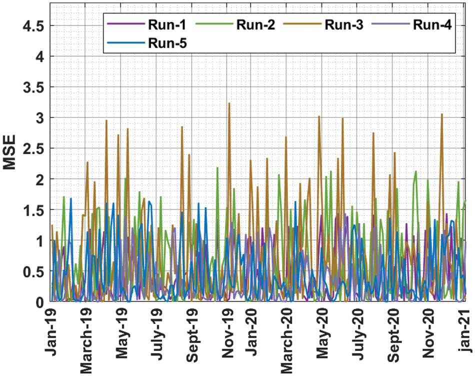
Figure 4: Result analysis of COMFO-DLRP technique with distinct runs

The results show that the COMFO-DLRP technique has resulted in enhanced performance with minimal values of MSE under all runs and seasons. For instance, on Jan-19, the COMFO-DLRP technique has obtained least MSE of 0.369713, 0.496275, 0.512775, 0.311138, and 0.385938 under runs 1-5 respectively. In Addition, on Apr-19, the COMFO-DLRP system has obtained lower MSE of 0.257575, 0.434113, 0.934613, 0.310125, and 0.813313 under runs 1–5 correspondingly. Moreover, on Aug-19, the COMFO-DLRP algorithm has reached least MSE of 0.438625, 0.547938, 0.836313, 0.232250, and 0.464363 under runs 1–5 respectively. Furthermore, on Jan-20, the COMFO-DLRP technique has gained minimum MSE of 0.317750, 0.679450, 0.681100, 0.296788, and 0.218913 under runs 1–5 correspondingly. Besides, on Apr-20, the COMFO-DLRP technique has obtained least MSE of 0.570638, 0.774675, 0.961300, 0.415550, and 0.240263 under runs 1–5 correspondingly. Along with that, in Jul-20, the COMFO-DLRP methodology has attained minimum MSE of 0.242688, 0.787375, 0.511400, 0.414500, and 0.369000 under runs 1–5 respectively. Meanwhile, on Oct-20, the COMFO-DLRP technique has gained least MSE of 0.465150, 0.550788, 0.886175, 0.471475, and 0.743463 under runs 1–5 correspondingly. Finally, on Jan-21, the COMFO-DLRP methodology has obtained least MSE of 0.465150, 0.768313, 0.147163, 0.240263, and 0.374338 under runs 1–5 correspondingly.

Tab. 2 provides a brief comparative rainfall forecasting outcomes of the COMFO-DLRP technique with other methods interms of MSE and root mean square error (RMSE) [24]. The table values highlighted that the COMFO-DLRP technique has resulted in effectual outcomes with minimal values of MSE and RMSE.

Fig. 5 provides a comparative MSE examination of the COMFO-DLRP technique with recent methods. The results indicated that the MLP model has resulted in ineffectual outcomes with higher MSE of 7.73285. Followed by, the 1-DCNN and LSTM models have obtained slightly reduced MSE of 5.24135 and 5.33379 respectively. Moreover, the deep and wide rainfall prediction model (DWRPM) technique has resulted in to even decreased MSE of 4.71585. However, the COMFO-DLRP technique has accomplished superior results with the least MSE of 0.35260.

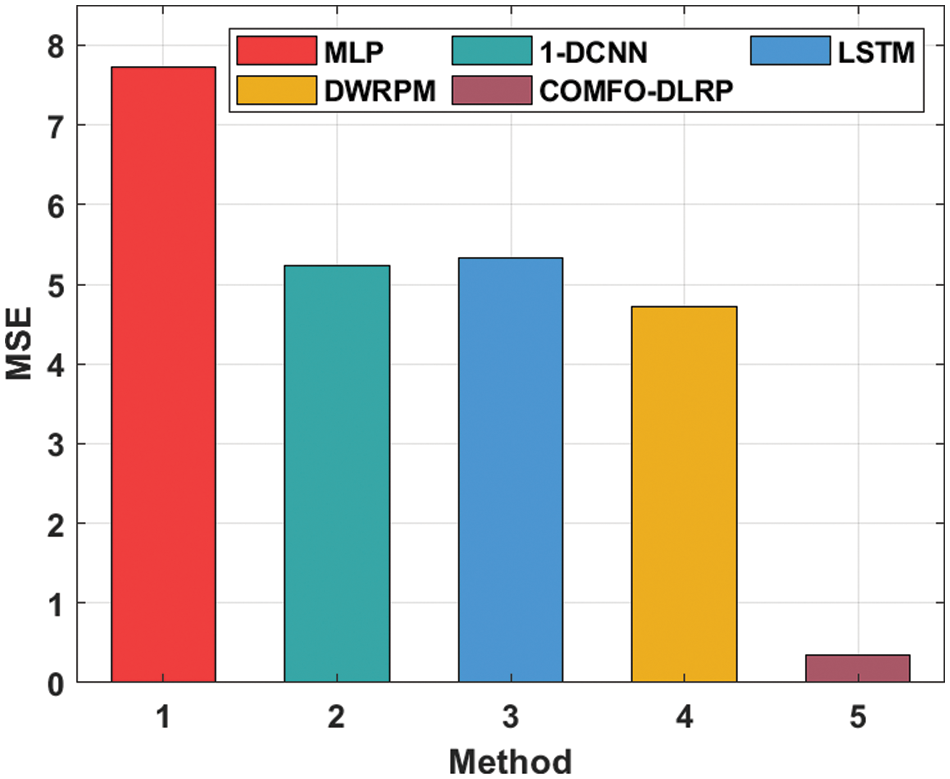
Figure 5: MSE analysis of COMFO-DLRP technique with recent approaches

Fig. 6 offers a comparative RMSE examination of the COMFO-DLRP approach with recent methods. The results referred that the MLP technique has resulted in ineffectual outcomes with superior RMSE of 2.78080. Likewise, the 1-DCNN and LSTM methodologies have gained slightly reduced RMSE of 2.28940 and 2.30950 correspondingly. Eventually, the DWRPM technique has resulted in even decreased RMSE of 2.17160. At last, the COMFO-DLRP methodology has accomplished superior outcomes with the minimum RMSE of 0.59380.

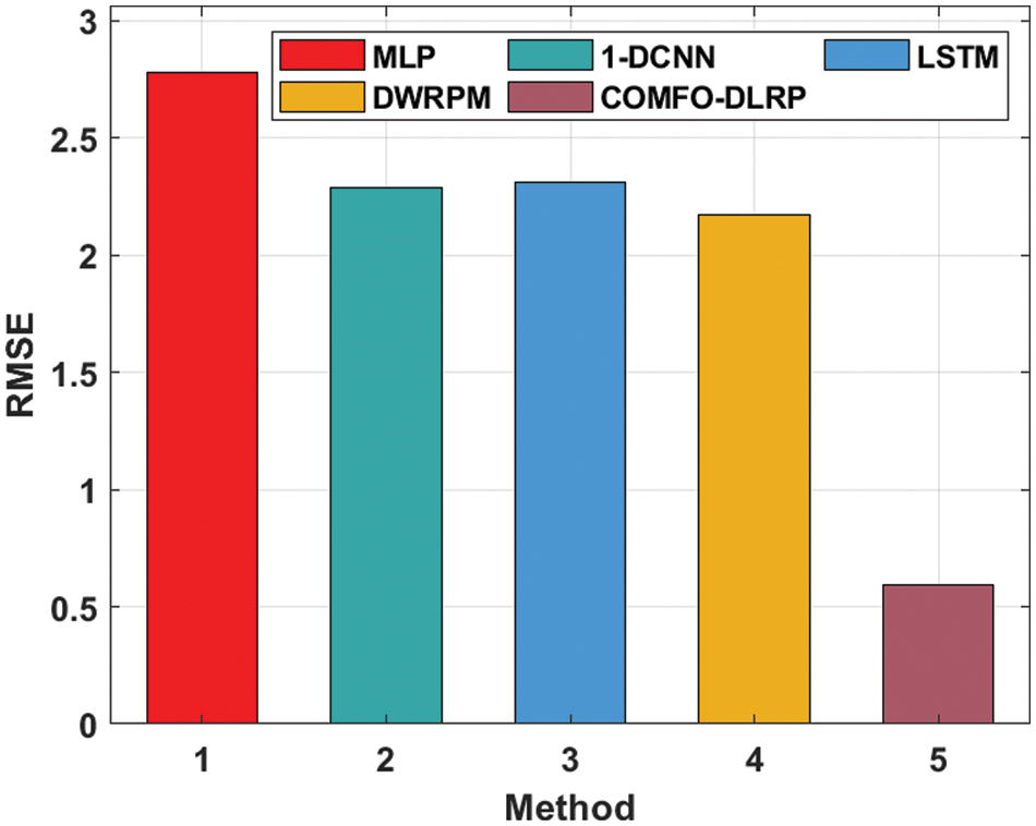
Figure 6: RMSE analysis of COMFO-DLRP technique with recent approaches

From the result analysis, it is ensured that the COMFO-DLRP technique has effectively forecasted the rainfall over the other techniques.

5  Conclusion

In this study, a novel COMFO-DLRP algorithm was developed to predict rainfall and thereby determine environmental changes. The presented COMFO-DLRP technique encompasses a series of processes namely data pre-processing, CM based feature selection, DBN based prediction, and COMFO based hyperparameter tuning. The COMFO algorithm is designed by incorporating the concepts of COBL with MFO algorithm. For inspecting the improved performance of the COMFO-DLRP approach, a comprehensive experimental analysis was performed and the outcomes are assessed under various measures. The simulation outcome highlighted the improved outcomes of the COMFO-DLRP method on the other techniques. Therefore, the COMFO-DLRP technique has the ability to attain improved predictive outcomes. In future, metaheuristics based feature selection algorithms can be derived to boost the classification results.

Funding Statement: The authors extend their appreciation to the Deanship of Scientific Research at King Khalid University for funding this work under grant number (RGP 2/180/43). Princess Nourah bint Abdulrahman University Researchers Supporting Project number (PNURSP2022R235), Princess Nourah bint Abdulrahman University, Riyadh, Saudi Arabia. The authors would like to thank the Deanship of Scientific Research at Umm Al-Qura University for supporting this work by Grant Code: (22UQU4270206DSR01).

Conflicts of Interest: The authors declare that they have no conflicts of interest to report regarding the present study.

References

 1.  A. Dogan and D. Birant, “Machine learning and data mining in manufacturing,” Expert Systems with Applications, vol. 166, no. 2, pp. 114060, 2021. [Google Scholar]

 2.  P. E. Cruz, R. Godina and E. M. G. Rodrigues, “A review of data mining applications in semiconductor manufacturing,” Processes, vol. 9, no. 2, pp. 305, 2021. [Google Scholar]

 3.  D. Shin and J. Shim, “A systematic review on data mining for mathematics and science education,” International Journal of Science and Mathematics Education, vol. 19, no. 4, pp. 639–659, 2021. [Google Scholar]

 4.  A. Namoun and A. Alshanqiti, “Predicting student performance using data mining and learning analytics techniques: A systematic literature review,” Applied Sciences, vol. 11, no. 1, pp. 237, 2020. [Google Scholar]

 5.  A. Khan and S. K. Ghosh, “Student performance analysis and prediction in classroom learning: A review of educational data mining studies,” Education and Information Technologies, vol. 26, no. 1, pp. 205–240, 2021. [Google Scholar]

 6.  Y. Xiang, L. Gou, L. He, S. Xia and W. Wang, “A SVR-ANN combined model based on ensemble EMD for rainfall prediction,” Applied Soft Computing, vol. 73, no. 2002, pp. 874–883, 2018. [Google Scholar]

 7.  J. D. Sierra and M. del Jesus, “Long-term rainfall prediction using atmospheric synoptic patterns in semi-arid climates with statistical and machine learning methods,” Journal of Hydrology, vol. 586, pp. 124789, 2020. [Google Scholar]

 8.  Y. Dash, S. K. Mishra and B. K. Panigrahi, “Rainfall prediction for the Kerala state of India using artificial intelligence approaches,” Computers & Electrical Engineering, vol. 70, pp. 66–73, 2018. [Google Scholar]

 9.  R. Kumar, M. P. Singh, B. Roy and A. H. Shahid, “A comparative assessment of metaheuristic optimized extreme learning machine and deep neural network in multi-step-ahead long-term rainfall prediction for all-indian regions,” Water Resources Management, vol. 35, no. 6, pp. 1927–1960, 2021. [Google Scholar]

10. S. Sharadqah, A. M. Mansour, M. A. Obeidat, R. Marbello and S. M. Perez, “Nonlinear rainfall yearly prediction based on autoregressive artificial neural networks model in central jordan using data records: 1938–2018,” International Journal of Advanced Computer Science and Applications, vol. 12, no. 2, pp. 240–247, 2021. [Google Scholar]

11. D. Sun, J. Wu, H. Huang, R. Wang, F. Liang et al., “Prediction of short-time rainfall based on deep learning,” Mathematical Problems in Engineering, vol. 2021, no. 5, pp. 1–8, 2021. [Google Scholar]

12. W. M. Ridwan, M. Sapitang, A. Aziz, K. F. Kushiar, A. N. Ahmed et al., “Rainfall forecasting model using machine learning methods: Case study Terengganu, Malaysia,” Ain Shams Engineering Journal, vol. 12, no. 2, pp. 1651–1663, 2021. [Google Scholar]

13. D. Endalie, G. Haile and W. Taye, “Deep learning model for daily rainfall prediction: Case study of Jimma Ethiopia,” Water Supply, pp. ws2021391, 2021. [Google Scholar]

14. R. Venkatesh, C. Balasubramanian and M. Kaliappan, “Rainfall prediction using generative adversarial networks with convolution neural network,” Soft Computing, vol. 25, no. 6, pp. 4725–4738, 2021. [Google Scholar]

15. D. Z. Haq, D. C. R. Novitasari, A. Hamid, N. Ulinnuha, Y. Farida et al., “Long short-term memory algorithm for rainfall prediction based on El-Nino and IOD data,” Procedia Computer Science, vol. 179, no. 1, pp. 829–837, 2021. [Google Scholar]

16. F. Zhang, X. Wang, J. Guan, M. Wu and L. Guo, “RN-Net: A deep learning approach to 0-2 h rainfall nowcasting based on radar and automatic weather station data,” Sensors, vol. 21, no. 6, pp. 1981, 2021. [Google Scholar]

17. M. A. B. Rhaiem, A. B. Hassine, A. Ouertani and I. R. Farah, “A hybrid rainfall prediction model for tunisian agriculture regions based on osm data, voronoi spatial analysis and long short term memory deep learning,” in EGU General Assembly Conf. Abstracts, pp. EGU21–12993, 2021. [Google Scholar]

18. E. O. Omuya, G. O. Okeyo and M. W. Kimwele, “Feature selection for classification using principal component analysis and information gain,” Expert Systems with Applications, vol. 174, pp. 114765, 2021. [Google Scholar]

19. S. M. Mujeeb, R. P. Sam and K. Madhavi, “Trust and energy aware routing algorithm for Internet of Things networks,” International Journal of Numerical Modelling: Electronic Networks, Devices and Fields, vol. 34, no. 4, pp. e2858, 2021. [Google Scholar]

20. R. A. Khurma, I. Aljarah and A. Sharieh, “A simultaneous moth flame optimizer feature selection approach based on levy flight and selection operators for medical diagnosis,” Arabian Journal for Science and Engineering, vol. 46, no. 9, pp. 8415–8440, 2021. [Google Scholar]

21. M. G. Arani, A. Souri, F. Safara and M. Norouzi, “An efficient task scheduling approach using moth-flame optimization algorithm for cyber-physical system applications in fog computing,” Transactions on Emerging Telecommunications Technologies, vol. 31, no. 2, pp. e3770, 2020. [Google Scholar]

22. H. R. Tizhoosh, “Opposition-based learning: a new scheme for machine intelligence,” in Int. Conf. on Computational Intelligence for Modelling, Control and Automation and Int. Conf. on Intelligent Agents, Web Technologies and Internet Commerce (CIMCA-IAWTIC’06), Vienna, Austria, 1, pp. 695–701, 2005. [Google Scholar]

23. M. A. Elaziz and I. Attiya, “An improved Henry gas solubility optimization algorithm for task scheduling in cloud computing,” Artificial Intelligence Review, vol. 54, no. 5, pp. 3599–3637, 2021. [Google Scholar]

24. V. Bajpai, A. Bansal, K. Verma and S. Agarwal, “Prediction of rainfall in rajasthan, india using deep and wide neural network,” 2010. [Online]. Available: https://arxiv.org/abs/2010.11787. [Google Scholar]