Vehicle Detection in Challenging Scenes Using CenterNet Based Approach

1  Introduction

Human brain can recognize the objects and their orientation without a hitch by scrutinizing at a scene in an image. Evolution in the sector of deep learning and computer vision, gives us incentive that the higher-level tasks for instance scene understanding can be done effectively. Development in the field of computer vision specifically digital image processing techniques become strong asset in enabling many important Intelligent Transport System (IT’s) applications and components such as Advanced Driver-Assistance Systems (ADAS’s), traffic and activity monitoring, Automated Vehicular Surveillance (AVS), traffic behavior analysis last but not the least traffic management among others. Tiny-Vehicle Recognition (TVR) is of incredible interest in these applications, inferable from elevated safekeeping worries in IT’s. Traffic surveillance cameras on road sides and on signals are not of very good quality, so to recognize a vehicle that is far from camera (seems tiny) it’s difficult to capture and precisely recognize vehicle from low quality image, which increment number of road accidents. For surveillance, traffic monitoring and to count the number of Vehicles accurately on the road it is essential to recognize the small vehicles to do some useful task. There are number of research work has been done in this field such as in 2015 He et al. proposed Faster R-CNN [1] which incorporates Region Proposal Network (RPN) with the candidate extractor Region Of Interest (ROI). This technique show good recognition performance for objection detection benchmark COCO [2] and Pascal VOC [3] but for KITTI [4] vehicle detection benchmark, its performance was not well and achieved 56.39% mAP only. Due to large variation of scale RPN ignore small objects. In [5] proposed a technique which handles vehicle detection occlusion by overlapping vehicle segmentation. It was a vision based approach which utilizes some geometric features and elliptic characteristics to localize vehicles from overlapped occlusion blob. In this model occluded vehicles are extracted on the bases of external properties. As compare to [6] this model improves the accuracy by 22.9%. In [7] the developed model DP-SSD, a single deep neural network for vehicle detection which concatenates the feature pyramid of conventional SSD and adjusts the scales of default box small vehicles more accurately whereas the proposed model can localize only two classes accurately e.g., Car and Van with 82.11% accuracy. By increases the sample size to the model the problem of overfitting encounters also increase more false positive results [8] Also could not recognize the vehicle in challenging conditions. [9] Addressed the problem of large-scale variance and object occlusion this method showed good performance in recognition of smaller and larger objects whereas for shallow features from larger scales are not incorporated accurately. [10,11] also highlight some issues regarding vehicle detection.

Many issues still need to be tackle in Vehicle detection such as detecting very small vehicle from complex scene [9] such as in Fig. 1. Recognizing vehicle in different weather conditions, like partially occluded, variant scale, and contrast is the challenging task. So, there is need to develop such technique which can localize small vehicles in complex scenes such as different lightning conditions, weather conditions, recognizing even when half vehicle is not visible, multiple vehicles with different sizes. The proposed model’s general pipeline is shown below in Fig. 2. Contributions of our proposed work are as follows:

•   This research focuses on the detection of tiny vehicles in complex scenes to localize small vehicles accurately though CenterNet with different backbones.

•   This paper enables researcher to analyze the behavior of CenterNet with different backbones and best performance comparison between one-step model CenterNet with MSSD300* and SMOKE.

•   SOTA technology is proposed to provide high detection rate compared to previous vehicle detection methods on KITTI dataset.

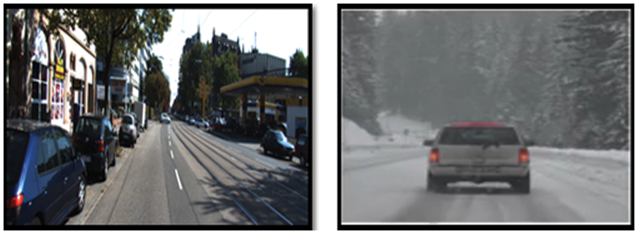
Figure 1: Tiny vehicle in complex scene

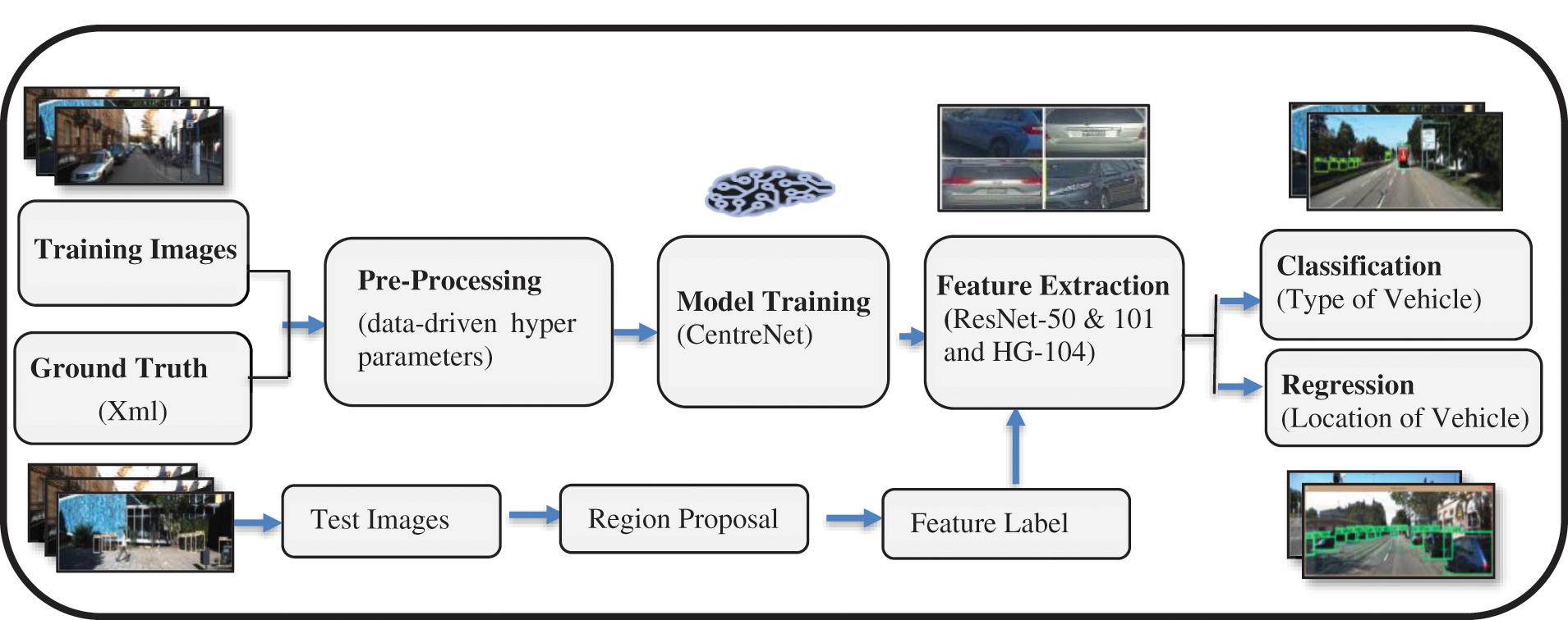
Figure 2: General pipeline of proposed model

The paper is classified in six sections as follows. In Section 2 related work is introduced, Than proposed methodology is elucidated in detail in Section 3, In Section 4 proposed methodology is scrutinize with different backbones, afterwards Results are discussed and compared with SOTA techniques to certify the proposed method’s performance in Section 5, Last but not the least whole in Section 6 paper is concluded.

2  Related Work

2.1 MSSD30000*

A single-Step detector based on DNN and object detection regression method which can localize and classify object in single forward pass. A forward pass calculates values of each output layer by traversing all the layers from first to the last. MSSD300* [12] takes the idea of anchor from RCNN and regression from YOLO (You Only Look Once) [13]. Anchors are the pre-computed, fixed size Bounding Boxes which are really close to original ground truth. So multiple bounding boxes are generated during forward pass of MSSD300* which is then prune by a threshold value to retain only likely prediction this technique is called non-maximum suppression. Early layers are responsible for generating classification of images in high quality. Next to perform detection at the end of back bone, we concatenate feature layer of convolution to produce detection at multiple scales as a result at each feature layer convolution network predicts detection.

2.2 SMOKE

SMOKE stands for Single-Stage Monocular 3D Object Detection via Keypoint Estimation. A 3D detector which predicts 3-dimensional bounding box against respective detected object by concatenating regressed 3D variable with single estimated keypoint. SMOKE [14] projects the 3D bounding box as a point on 3D cuboid center with size, distance and yaw as additional properties. Basically, targeted towards monocular images (both eyes are used separately) and proposed disentangle L1 loss to weigh dissimilar loss together in order to reduce the convergence of loss. In the beginning all the objects whose projected centers are out of image range are prune out. Then data augmentation is performed consisting random scale, horizontal flip and shift on heatmap. The output of final feature map is than down-sampled tetrad times corresponding to image (original) afterwards Group Norm is applied instead of Batch Norm as it is more sensitive to noise. At each feature map regression is applied channel wise to preserve consistency. The network is train with backbone DLA-34 and gives 85.62% mAP.

[1] Worked on Tiny-Vehicle detection for which a BFEN (Backward Feature Enhancement Network) is presented and exemplified, the research technique is particularly effectual to initiate high recall proposals. Combining a basic network with preserved spatial layout gives a notable performance boost. The proposed method works well on ‘hard’ subset of KITTI dataset and achieve the accuracy of 78.10%.

3  Methodology

This section elaborates the working principle of single-step based vehicle detection models. We used single step model CenterNet [15] with different backbones HourGlass [16], ResNet-50, ResNet-101 [17] architectures for vehicle detection. To make best comparison between speed and accuracy we evaluate our hypothesis on SOTA one-step model MSSD300* [12] (InceptionV2s, mobileNet, ResNet101) and SMOKE [14] with varying backbones because these model outperforms in object detection. To optimize the model we use Adam optimizer.

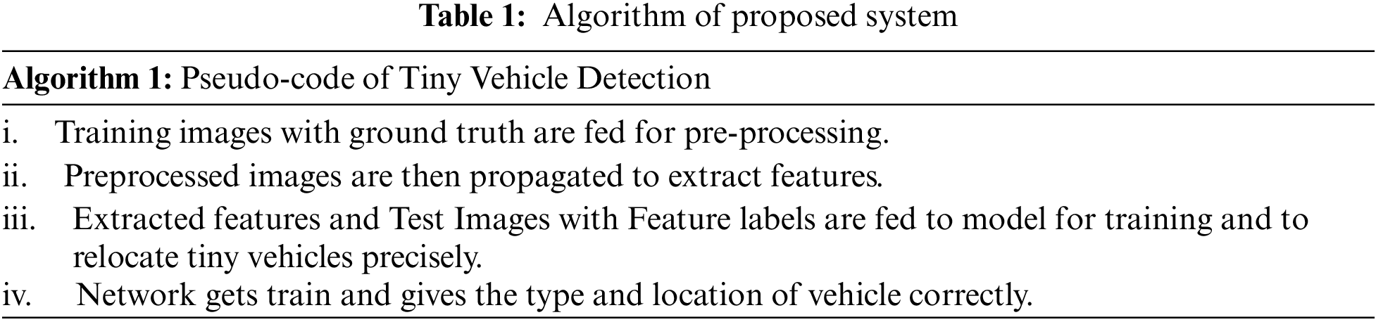
The information about vehicle is stored in the form of colored RGB images. There are multiple steps to detect and localize vehicle as expressed in Fig. 2. Pre-processing the training data is the initial step which include cleaning, contrast stretching and noise removal. Preprocessed data is then used to extract various types of features such as Type, size, and shape. Model is trained based on Features that are extracted so this step involves Model Learning. After model learning, the data is then classified and regressed which ultimately gives “Vehicle Type” and “Location of Vehicle in an image” respectively. The Proposed model shows the following steps.

Step 1: Input Image

KITTI vehicle detection benchmark is used in this detection and recognition framework, consisting 7481 images in “jpg” format having 1242 × 375 × 3 dimensions. There are various types of vehicles images in different sizes. Further explanation about the nature and classes of dataset is explained in Section 5.

Step 2: Pre-Processing

Despite the great success of Machine learning (ML) in many fields for instance computer vision, Natural Language Processing (NLP) etc. However, it is very arduous for novice programmers to apply ML adequately; they must decide between dozens of available ML algorithms and pre-processing methods and adjust the hyper parameters of the selected approaches for the dataset in hand. Adopting the right method leads state-of-the-art performance, but the need for these tedious manual tasks constitutes a substantial burden on real-world machine learning applications. With ever-increasing industrial uses of machine learning, now a strong demand for robust ML systems which perform inference autonomously on a given dataset recent automated machine learning (AutoML) systems find the right algorithm and data-driven hyper parameters without any human intervention. In Fig. 3 input image and image after pre-processing is shown.

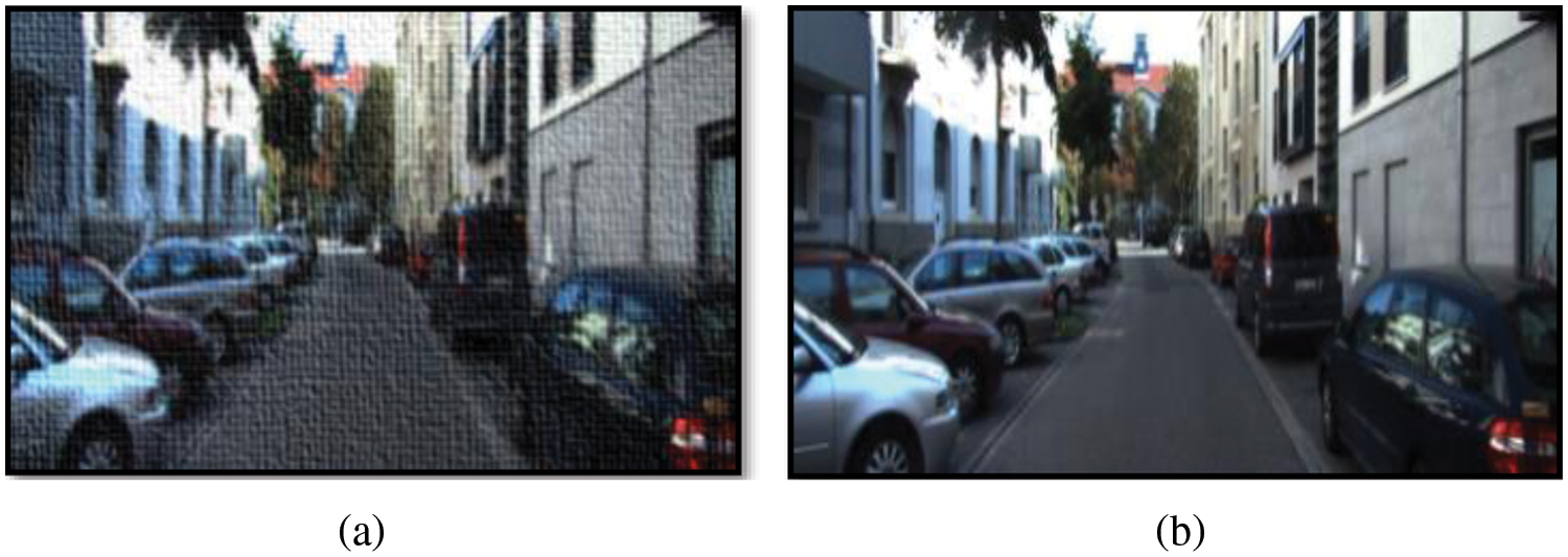
Figure 3: (a) Input image (b) pre-processed image

Step 3: Feature Extraction

The major component of deep learning is to extract useful features to clearly define vehicle in the image. Features are the properties which are input to deep learning model to predict and classify a vehicle; features are input to identify it. Precision of detection depends on the chosen features Fig. 4 shows the extracted features. In this research we use two feature extractors ResNet-50, ResNet-101 and HourGlass-104.

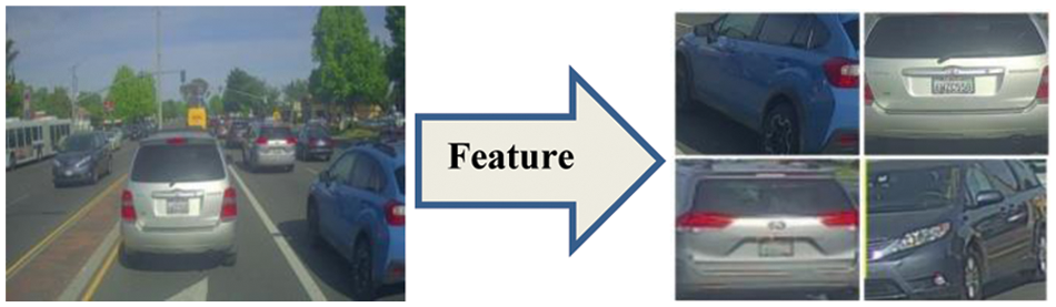
Figure 4: Feature extraction

Step 4: Model Training

At this stage extracted features are then passed to model for training. Model depicts the association between vehicles and its corresponding classes of vehicles. Here CenterNet model is used to train the KITTI Vehicle Detection Benchmark to resolve the issue of tiny vehicle.

Step 5: Classification and Regression

After successful training vehicles are classified by the model and gives detected vehicle with bounding box as shown in Fig. 5. Algorithm of pipeline is shown in Tab. 1.

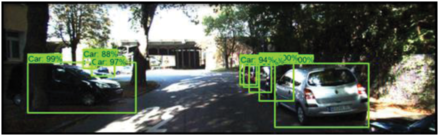
Figure 5: Classification and regression of vehicle

3.1 CenterNet

CenterNet is a type of one-step detector, established on deep neural network (DNN), an anchor free approach to regress and classify objects. In this approach center of the box is considered as object which also known as key points then this predicted center is used to get coordinates of the bounding box. When an image is passed via Fully Convolutional Network the final feature map gives heatmaps for each corresponding key point. In Fully Convolutional Network every input of one layer is connected to the each activation unit of the next layer. The crests of the heatmap depict predicted centers. Network generates width and height of each center whereas each predicted center have distinctive box width and height also in in post processing Non-Maximal suppression (NMS) [18] property because of this tightly coupled has been removed which reduces false positive results.

Having a look on overall workflow of the model we can see in Fig. 6 each forward pass from the framework three heads are predicted. Consider an “I” representing image with “W” depicting width and height H having three numbers of channels. Final dimension of the given heads will be decided by output stride R e.g., R = 4. Number of classes is shown as C. All heads have same height (H/R) and width (W/R) however distinct C values. Decisive head dimensions for input dimension 375x1225 with stride R = 4 would be 94x306 (H/R, W/R, C)-> (94, 306, 10) as shown in Fig. 6 .

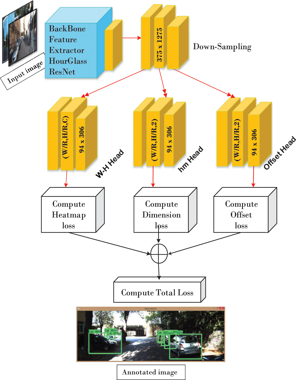
Figure 6: CenterNet architecture

3.2 Heatmap Head

Heatmap head is responsible for key point approximation of given image. To splat box center Gaussian Kernel is used, in order to produce ground truth heatmaps for estimation of loss propagation. n, m, o is the function of Y_hat heatmap. Y is the key point heatmap, n and m are coordinate offset. σ is object size adaptive standard deviation. p~ is the low-resolution equivalence of centers. In Eq. (2) if the Gaussian of two classes are overlapping then element-wise maximum will be done in order to find target class.

Ynmo=exp⁡(−(n−p~n)2+(m−p~m)22σp2)..(1)

 Ynmo{1=detectedcenterofparticularclass0=considerasbackground(2)

3.3 Dimension Head

Dimension head is used for dimension prediction of the box’s height and width. For object O in an image and class C having coordinates (x1, y1, x2, y2) then the regressed object’s size can be achieved through L1 distance norm S_O = (x2-x1 , y2-y1). Dimension for this Heatmap will be (W/R, H/R, 2). Whereas H and W are forecasted height and width of the box.

3.4 Offset Head

Offset Head is responsible to redeem the errors occurred during downsampling in an input image. Prediction of the center points are in discrete values which further need to map downsampled coordinates of processed image to higher dimensional input image. This procedure compromises original image pixel indices hence value disturbance occurs. To cope up this issue local Offset O_hat are shared between present objects in an image. The head dimensions (W/R, H/R, 2) whereas W and H are coordinate offset. After generating Heatmaps loss of each will be computed. For Heatmap Head following formula Eq. (3) is used to compute loss. When predicted Y^ is closer to 1 then weightage of generated loss will be decrease. Whereas if Y^ is not closer to 1 than the value of slope will be increase by the parameter α. In other case if Y^ is closer to 0 than [Y^_nmo] ∧α  makes overall loss 0. In Equation α Is the slope value parameter [Y] _nmo is Heatmap head and N is total Heatmap generated.

Lk=−1N∑nmo{(1−Y^nmo)αlog⁡Y^nmoif  Y^nmo=1(1−Y^nmo)β(Y^nmo)αotherwiselog⁡(1−Y^nmo)(3)

L1 Norm is used to compute predicted Offset Loss. Q^p^ is predicted offset and pR is ground truth offset. N is the Total Heatmap generated. Following Eq. (4) is used to calculate Offset Loss.

Loff=1N∑p|Q^p^−[pR−p^]|(4)

As discuss above due to downsampling of input in prediction step value disturbance occurs so to compute the original dimensions of the object again Loss L1 Norm is computed. Eq. (5) represents the mathematical representation of loss accumulation formula Given by D^pk are predicted dimensions where as Dk is the ground truth sizes given by.

Lsize=1N∑k=0N|D^pk−Dk|(5)

To accumulate total loss of CenterNet following expression is used. λs=0.1 use to scale the loss on pixels. λoff=1 to scale the offset. Instead of directly using raw pixel coordinates we scale the loss by these constant values.

Ltotal=Lk+λs∗Lsize+λoff∗Loff(6)

4  Backbone Used with CenterNet

4.1 HourGlass

Hourglass network [16] is a feature extractor which takes input as an image and extracts features by deconstructing the image into feature matrix. This Feature matrix with Low spatial understanding is then combined with earlier layers having higher spatial understanding to get good understand where object lies in an image. As shown in the Fig. 6.

There are multiple cubes each having multiple layers, each layer has stack of operations such as in first cube convolution of 7 × 7 is performed on an input image followed by Batch Normalization then ReLu Activation function is applied. Next it is passed into Bottleneck layer shown in Fig. 7. A Bottleneck is a layer it reduces the channels of input by performing 1 × 1 convolution before and after 3 × 3 convolution to project back the original dimension. Output of Bottleneck layer is than duplicated, one goes to MaxPool to perform feature extraction other is attached to network later to perform decoding i.e., up sampling. Upcoming cubes have similar structure as first one except the first block in Fig. 7. This cube operation will repeat 4 times including first one then feature map is generated through the deepest Bottleneck Layers. At this time image reduced into matrix representing a ‘tensor’. After getting feature map we upsample (shown in the Fig 7) the tensor to make input and output image of same dimension So here element wise addition is performed between Bottleneck layer (duplicated layer in encoding stage) and up sampled feature layer. During decoding stages, each cube is again convolve with 1 × 1 kernel and duplicate to generate heatmaps, so addition is performed again here. Loss is computed at the end of each stage. This is a structure of single hourglass, in our research we use total 104 of similar layers.

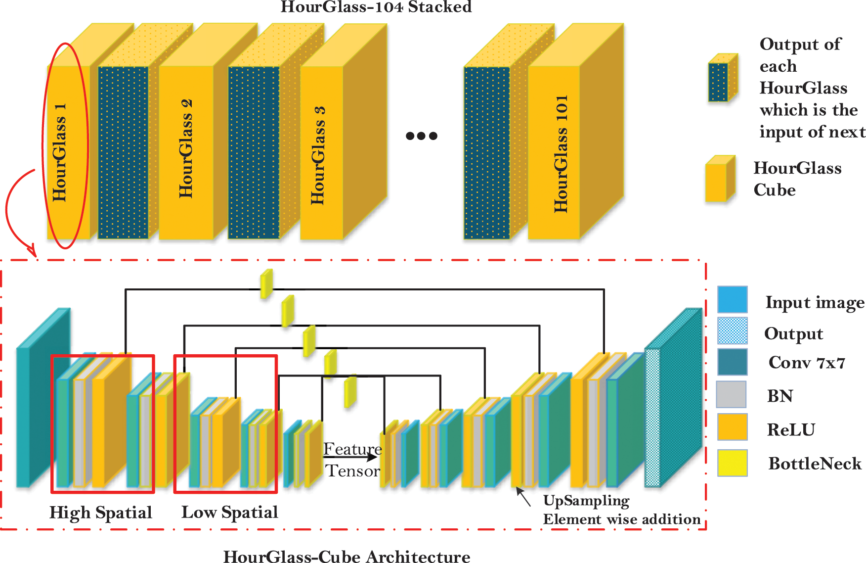
Figure 7: Hourglass feature detector architecture

4.2 ResNet

ResNet stands for Residual Network. It is another SOTA convolutional encoder-decoder network that extracts features from image. It consists of Identity connection that categorizes residual network, which takes the input directly to the end of each residual block known as Shortcut Connection as shown in the Fig. 7.

This helps to retrain the information compromised during processing of earlier layers. Mathematically, a ResNet block is a function of f(x) which by adding input x gives y, so that input and output dimensions become equal.

y=f(x)+X(7)

This architecture eradicates the problem of degradation, occurs when network’s depth increases so accuracy gets saturated. There are two versions of residual block [17] as shown in the Fig. 8. Block V1 is known as Residual Block comprising of two layers of 3 × 3 known as V1. ResNet v1 performs convolution followed by BN and ReLU activation function. In our research we evaluate ResNet-50 v1 as backbone with CenterNet. In Fig. 8 Bottleneck Block V2 comprises a stack of three layers of 1 × 1, 3 × 3 and 1 × 1 convolution. 1 × 1 is responsible for reducing the original dimension and then restoring the altered dimensions whereas 3 × 3 is bottleneck with reduced input\output dimensions which is known as V2. ResNet v2 first performs BN and ReLu activation followed by matrix convolution. In ResNet block –V1 addition operation of a Block (containing Convolution, BN, and ReLu) and Skip connection is followed by ReLU activation and then transferred to next Block as an input. Where as in ResNet-V2 addition function performed between residual block and short Connection is directly propagated to next block as an input.

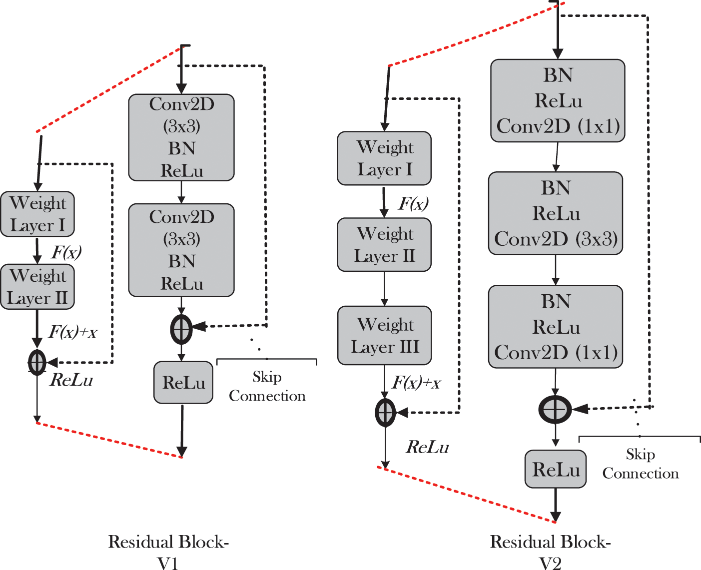
Figure 8: ResNet architecture

In our research we evaluate ResNet50-V1 with 512 × 512 FPN and ResNet-101-V1 with 512 × 512 which gives 62.08% and 79.20% mAP respectively. Then we evaluate ResNet50 and ResNet101 with Residual Block V2 in which we use Bottleneck Block with three up-sampling layers with 256,128,64 channels then add 3 × 3 deformable convolutional layer with corresponding up sampling layer which gives 75.20% and 92.60% mAP respectively. Then we use CenterNet with HourGlass-104 explained earlier in detail which shows 98.9% mAP.

5  Experimental Results

5.1 Dataset

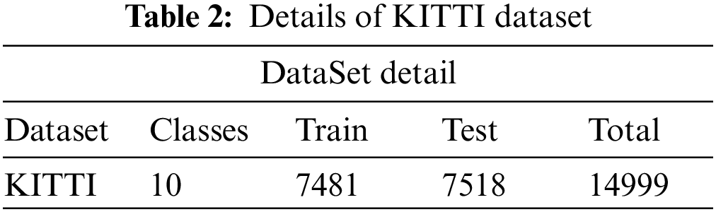
KITTI [4] vehicle detection benchmark dataset is used in this detection and recognition framework, consisting 7481 images in “jpg” format having 1242 × 375 × 3 dimensions. Tab. 2 shows the details of dataset. Minimum bounding box height is 25 pixels whereas the max occlusion level is difficult to see. We used KITTI benchmark as it cover vehicles of different sizes and types as compared to other datasets, also dataset contains occluded vehicles that are difficult to see which is the concerned problem of our research. In original KITTI benchmark there are total eight classes Car, Person_sitting, Van, Pedestrian, Truck, Cyclist, Tram, Misc or DontCare. Apart from these we have included two more classes, also changed naming convention while annotation. In benchmark there were classes which were not of our concern for instance Pedestrian, Person_sitting, Cyclist, so we annotated benchmark to produce annotation according to our own need, newly annotation consists of ten classes which includes Car, Van, Truck, Carriage, Crane, Cycle, Tram, Bus, MotorCycle and DontCare. DontCare class consists of annotation of those images which do not belongs to any of the above class specially sign boards having vehicle image. Images are from blurry to medium quality.

5.2 Evaluation Measure

We have evaluated proposed method by using the different evaluation metrics i.e., Accuracy, Precision, Recall and mAP. Accuracy is being evaluated by computing mAP (mean average precision-recall curve). mAP is a prediction among Positive anchor boxes (predicted by model) and Ground-truth anchor boxes (actual boxes given to model). Mathematically, it can be represented as following TP are outcome where model correctly predict positive classes, In TN model correctly predict negative classes. FP shows incorrect prediction of positive classes. In FN model incorrectly predict negative. N is total number of classes in our case N = 10.

Recall=TPPredicted ResultsorTPTP=FN(8)

mAP =1N∑i=1NAPiorTP+TNTotal(9)

5.3 Model Evaluation

We chose one-stage CenterNet as a base network detector with three dissimilar Feature Extractor ResNet-50, ResNet-101 and HourGlass-104 as backbones for experiment. The good reason to choose ResNet feature extractor as backbone because stacking a residual layer is easier to map without degrading the performance of the network [19] and HourGlass-104 recently purposed network for the first time used to detect vehicles. After successful training of model with all three backbones, model become able to identify and recognize vehicle successfully. Our network is pre-trained on MS-COCO [2]. We train our model on KITTI Benchmark with 70k steps. Fig. 12 shows the localization results of vehicle, with 98.9% value of mAP. We can say that CenterNet HourGlass-104 is one of the models which is suitable for detection problem even when dataset is not in high quality. CenterNet-ResNet-101 shows good results with real time speed of 0.1 s per image with 92.60%. Here are some clicks of test data with correctly detected even tiny vehicles.

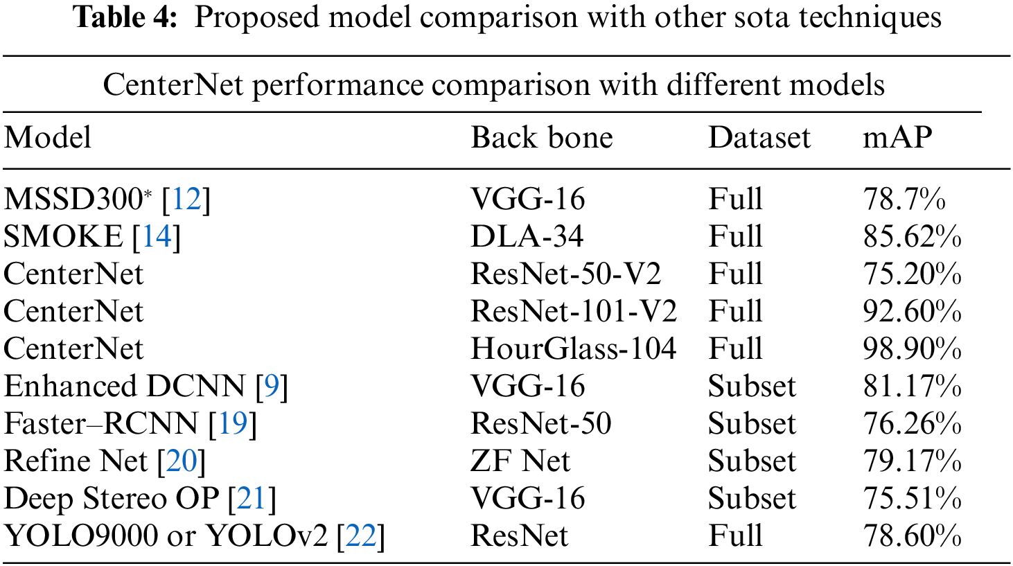
Among One-stage detectors CenterNet Outperforms in detection task and take less time as compare to other Deep learning techniques as shown in Fig. 10. All the models are of one-step and are trained on KITTI dataset to make evaluation in true meaning. Betwixt the proposed backbones used with the CenterNet HourGlass-104 outperformed as shown in the Fig. 11. To validate our model’s performance, we also make comparison of CenterNet with Other SOTA models on KITTI Benchmark in Tab. 4 which clearly shows the performance improvement to 98.9% mAP. Some of the models are trained on subset wherein other are on whole dataset. Results of the training are shown as below in Tab. 4 depicting CenterNet-HourGlass-101 outplayed with 24.3% mAP from MSSD300* and 13.2% mAP from SMOKE.

6  Conclusion

This Research introduces and improves single-stage detector CenterNet in deep learning. The prime purpose of the research is to increase the detection rate of tiny vehicle to accurately identify small vehicle. The experiments were conducted on standard dataset having different view angles, weather condition, lightning conditions, and shadow scenes. To validate the performance, we compare our model with latest techniques MSSD300* and SMOKE on same dataset, our model beats the performance of real-time speed with high Mean Average Precision as shown in Tab. 3 and Fig. 9. Our technique eradicates the problem of tiny vehicle to great extent which is the huge challenge in MSSD300* [12]. Our model is single-pass, Fast and accurate and does not affect the output image dimension as offset heatmap maps the predicted coordinates to original through local offset, accumulated at early stage.

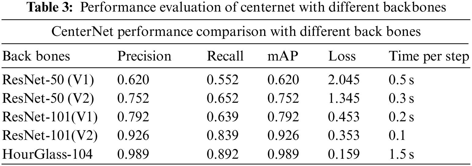
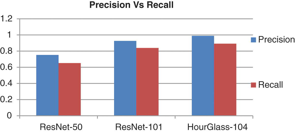
Figure 9: Precision vs. recall of CenterNet

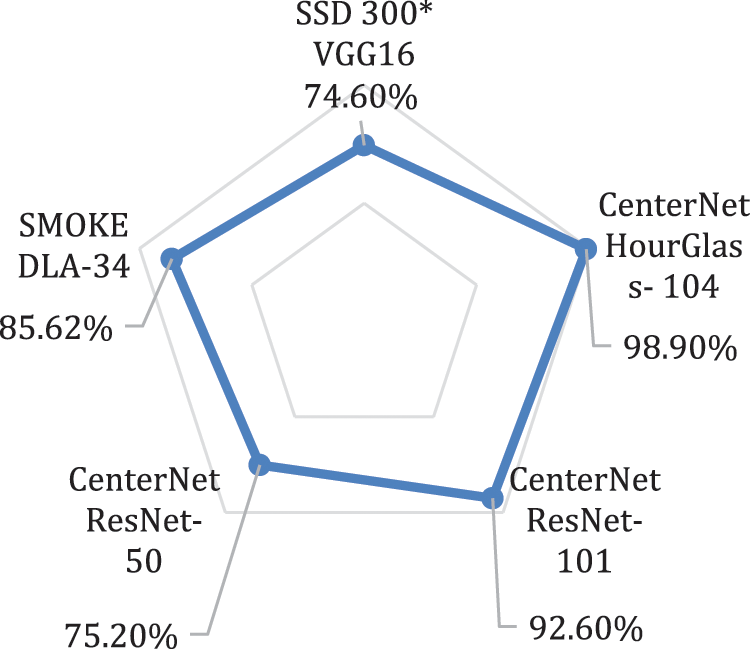
Figure 10: Comparison of different techniques

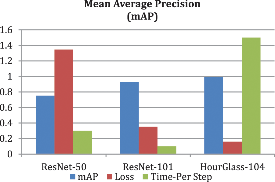
Figure 11: mAP of CenterNet with ResNet-50, 101 and HourGlass-104

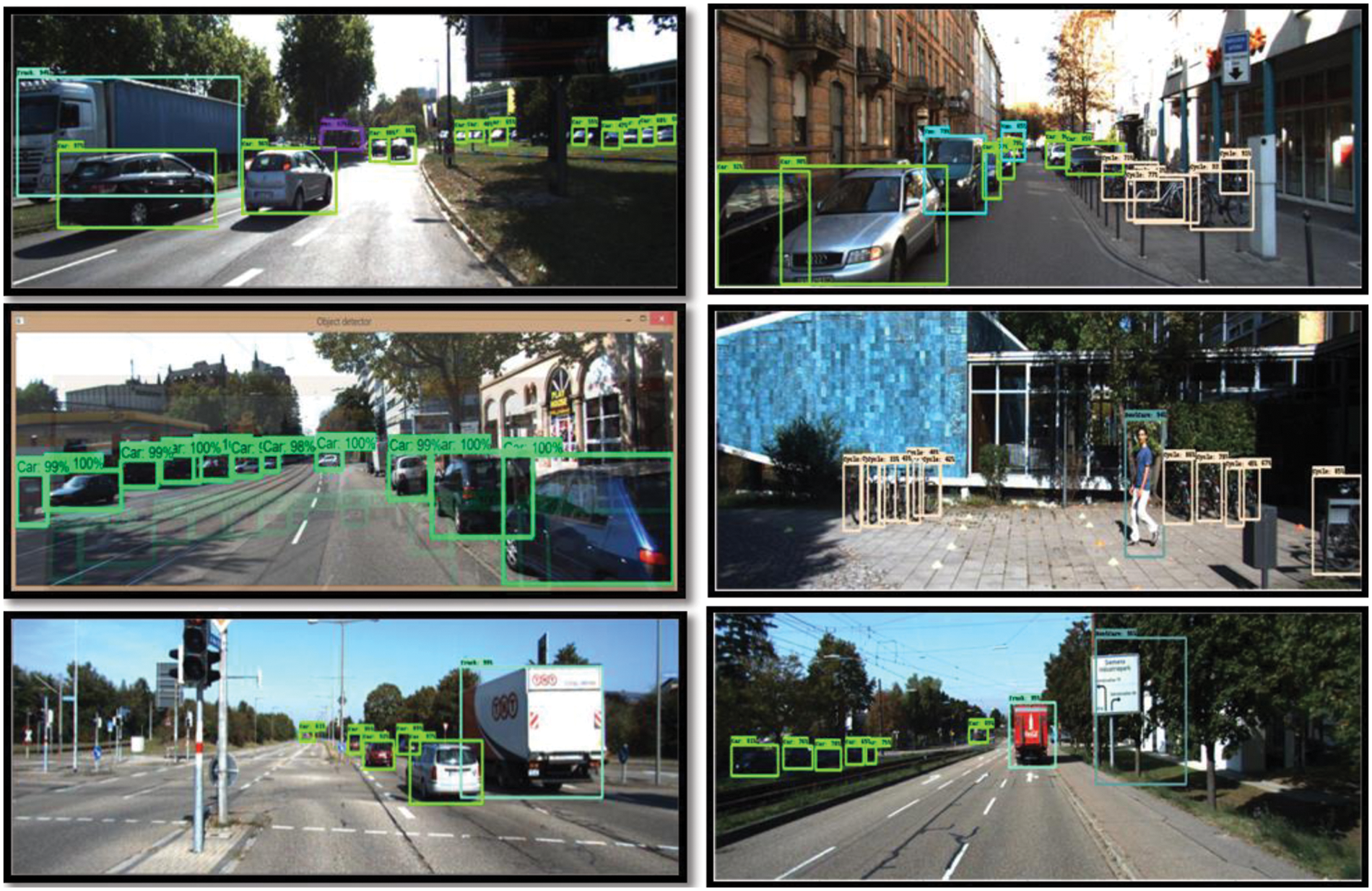
Figure 12: CenterNet detection result

Acknowledgement: We would like to thank for funding the publication of this project.

Funding Statement: The authors received no specific funding for this study.

Conflicts of Interest: The authors declare that they have no conflicts of interest to report regarding the present study.

References

 1.  W. Liu, S. Liao and W. Hu, “Towards accurate tiny vehicle detection in complex scenes,"Neurocomputing, vol. 347, pp. 24–33, 2019. [Google Scholar]

 2.  T. -Y. Lin, M. Maire, S. Belongie, J. Hays, P. Perona et al., “Microsoft coco: Common objects in context,” in European Conference on Computer Vision, Springer, Switzerland, pp. 740–755, 2014. [Google Scholar]

 3.  M. Everingham, L. Van Gool, C. K. Williams, J. Winn, and A. Zisserman, “The pascal visual object classes (voc) challenge,” International Journal of Computer Vision, vol. 21, no. 2, pp. 303–338, 2010. [Google Scholar]

 4.  A. Geiger, P. Lenz, C. Stiller and R. Urtasun, “Vision meets robotics: The KITTI dataset,” The International Journal of Robotics Research, vol. 32, no. 11, pp. 1231–1237, 2013. [Google Scholar]

 5.  H. N. Phan, L. H. Pham, D. N.-N. Tran and S. V.-U. Ha, “Occlusion vehicle detection algorithm in crowded scene for traffic surveillance system,” in 2017 Int. Conf. on System Science and Engineering (ICSSE), IEEE, Ho Chi Minh City, Vietnam, pp. 215–220, 2017. [Google Scholar]

 6.  S. V.-U. Ha, L. H. Pham, H. N. Phan and P. Ho-Thanh, “A robust algorithm for vehicle detection and classification in intelligent traffic system,” in 16th Asia Pacific Industrial Engineering & Management Systems Conference (APIEMS 2015), Ho Chi Minh City, Vietnam, pp. 1832–1838, 2015. [Google Scholar]

 7.  F. Zhang, C. Li and F. Yang, “Vehicle detection in urban traffic surveillance images based on convolutional neural networks with feature concatenation,” Sensors, vol. 19, no. 3, pp. 594, 2019. [Google Scholar]

 8.  L. Suhao, L. Jinzhao, L. Guoquan, B. Tong, W. Huiqian et al., “Vehicle type detection based on deep learning in traffic scene,” Procedia Computer Science, vol. 131, pp. 564–572, 2018. [Google Scholar]

 9.  J. Wei, J. He, Y. Zhou, K. Chen, Z. Tang et al., “Enhanced object detection with deep convolutional neural networks for advanced driving assistance,” IEEE Transactions on Intelligent Transportation Systems, vol. 21, no. 4, pp. 1572–1583, 2019. [Google Scholar]

10. C.-C. Tsai, C.-K. Tseng, H.-C. Tang and J.-I. Guo, “Vehicle detection and classification based on deep neural network for intelligent transportation applications,” in 2018 Asia-Pacific Signal and Information Processing Association Annual Summit and Conference (APSIPA ASC), IEEE, Honolulu, HI, USA, pp. 1605–1608, 2018. [Google Scholar]

11. C. Donahue, J. McAuley and M. Puckette, “Synthesizing audio with generative adversarial networks,” arXiv preprint arXiv:1802.04208, 2018. [Google Scholar]

12. J. Fu, C. Zhao, Y. Xia and W. Liu, "Vehicle and wheel detection: A novel SSD-based approach and associated large-scale benchmark dataset,” Multimedia Tools and Applications, vol. 79, pp. 1–20, 2020. [Google Scholar]

13. J. Redmon, S. Divvala, R. Girshick and A. Farhadi, “You only look once: Unified, real-time object detection,” in Proc. of the IEEE Conference on Computer Vision and Pattern recognition, Las Vegas, 2016. [Google Scholar]

14. Z. Liu, Z. Wu and R. Tóth, “SMOKE: Single-stage monocular 3d object detection via keypoint estimation,” in Proc. of the IEEE/CVF Conf. on Computer Vision and Pattern Recognition Workshops, Virtual, pp. 996–997, 2020. [Google Scholar]

15. X. Zhou, D. Wang and P. Krähenbühl, “Objects as points,” arXiv preprint arXiv:.07850, 2019. [Google Scholar]

16. A. Newell, K. Yang and J. Deng, “Stacked hourglass networks for human pose estimation,” in European Conference on Computer Vision, Springer, Amsterdam, The Netherlands, pp. 483–499, 2016. [Google Scholar]

17. K. He, X. Zhang, S. Ren and J. Sun, “Deep residual learning for image recognition,” in Proc. of the IEEE Conference on Computer Vision and Pattern Recognition, Las Vegas, pp. 770–778, 2016. [Google Scholar]

18. R. Rothe, M. Guillaumin and L. Van Gool, “Non-maximum suppression for object detection by passing messages between windows,” in Asian Conference on Computer Vision, Springer, Singapore, pp. 290–306, 2014. [Google Scholar]

19. R. Girshick, “Fast r-cnn,” in Proc. of the IEEE International Conference on Computer Vision, Boston, pp. 1440–1448, 2015. [Google Scholar]

20. R. N. Rajaram, E. Ohn-Bar and M. M. Trivedi, “RefineNet: Iterative refinement for accurate object localization,” in 2016 IEEE 19th Int. Conf. on Intelligent Transportation Systems (ITSC), IEEE, Rio de Janeiro, Brazil, pp. 1528–1533, 2016. [Google Scholar]

21. C. C. Pham and J. W. Jeon, “Robust object proposals re-ranking for object detection in autonomous driving using convolutional neural networks,” Signal Processing: Image Communication, vol. 53, pp. 110–122, 2017. [Google Scholar]

22. J. Redmon and A. Farhadi, “YOLO9000: Better, faster, stronger,” in Proc. of the IEEE Conference on Computer Vision and Pattern Recognition, San Juan, pp. 7263–7271, 2017. [Google Scholar]