Automated Brain Tumor Diagnosis Using Deep Residual U-Net Segmentation Model

1  Introduction

Image Segmentation and classification were the widest image processing methods utilized for segmentation of the region of interest (ROI) and for dividing them into provided classes. Image classification and segmentation serve a significant role in multiple applications in extracting features, understanding images, and interpreting and analyzing them [1]. Computed Tomography (CT) scan and Magnetic Resonance Imaging (MRI) were utilized to examine and resection the abnormality relating to size shape, or position of brain tissue. Brain Tumor (BT) is regarded as a neoplastic and abnormal cell development from the brain [2]. Segmentation was a process of separation of an image to a similar class of properties like brightness, color, gray level, and contrast, to regions or blocks [3,4]. Brain tumor segmentation was used in medical imaging like magnetic resonance (MR) images or latest imaging modality for separating the tumor tissues like necrosis (dead cells) and edema from usual brain tissues, namely white matter (WM), gray matter (GM), and cerebrospinal fluid (CSF) [5]. For detecting tumor tissues from medical imaging modes, segmentation can be used, and based on the evaluations achieved with the help of enhanced medical imaging modalities, specialization in patient care was given to patients having BT [6]. The detection of a BT at initial level was the main problem to provide enhanced medication to the patient. After a BT has been suspected clinically, radiological assessment was needed for determining its size, place, and effects on the nearby regions [7]. It has been made clear that the survival chances of a tumor contaminated patient are raised when cancer has been identified at the initial level. So, the BTs study with the help of imaging modalities obtained significance in the radiological section [8].

From the study, it detected those conventional methods were more potential for the initial cluster centers and cluster size [9]. When such clusters differ with distinct early inputs, after which it creates issues in categorizing pixels. In the present general fuzzy cluster mean system, the cluster centroid value was considered randomly. It would rise up the duration to receive a favorable solution [10]. Manual evaluation and segmentation of MRI brain images performed by radiotherapists become tedious; the segmentation was performed with the help of machine learning (ML) methods whose calculation speed and accuracy were low.

Ilhan et al. [11] suggest an effective algorithm for segmenting the whole BTs through MRI images on the basis of tumor localization and advancement methodologies using deep learning (DL) structure called U-net. At first, the histogram related nonparametric tumor localization methodology was implied for localizing the tumorous zones and the presented tumor advancement technique can be utilized for modifying the localized zones for increasing the visual appearances of low-contrast or indistinct tumors. Raju et al. [12] recommend the automated technique of categorization with the help of the Harmony-Crow Search (HCS) Optimized system for training the multi-Support Vector Neural Network (SVNN) technique. The BT segmentation can be done with the help of the Bayesian fuzzy clustering technique, where the classification of tumors can be executed with the help of the suggested HCS Optimization system-related multi-SVNN classifier. Das et al. [13] in consideration of 32 attributes, together with clusters having performance evaluation metrics, AI architecture, clinical evaluation, imaging modalities, and hyper-parameters. Kapila et al. [14] proposed approach uses a potential approach for BT classification and segmentation. For classifying and segmenting the BT MR image through artificial neural network (ANN) and Modified Fuzzy C-Means (MFCM). At this point, the features that are extracted have been chosen optimally by Hybrid Fruit fly and artificial bee colony (HFFABC). In [15], the researchers were concerned about the issue of completely automated BT segmentation in multimodal MRI. Conversely applying classification over whole volume data that needs heavy load of both memory and computation, suggests a 2-stage technique.

This study introduces an Automated Deep Residual U-Net Segmentation with Classification model (ADRU-SCM) for Brain Tumor Diagnosis. The presented ADRU-SCM model majorly focuses on the segmentation and classification of BT. The presented ADRU-SCM model involves wiener filtering (WF) based pre-processing to eradicate the noise that exists in it. In addition, the ADRU-SCM model follows deep residual U-Net segmentation model to determine the affected brain regions. Moreover, VGG-19 model is exploited as a feature extractor. Finally, tunicate swarm optimization (TSO) with gated recurrent unit (GRU) model is applied as a classification model and the TSO algorithm effectually tunes the GRU hyperparameters. The performance validation of the ADRU-SCM approach was tested using FigShare dataset.

2  The Proposed Model

In this study, a novel ADRU-SCM technique was established for the segmentation and classification of BT. The presented ADRU-SCM technique primarily applies WF based pre-processing to eradicate the noise that exists in it. In addition, the ADRU-SCM model follows deep residual U-Net segmentation model to determine the affected brain regions. Moreover, VGG-19 model is exploited as a feature extractor. Finally, TSO with GRU model is applied as a classification model. Fig. 1 depicts the overall process of ADRU-SCM approach.

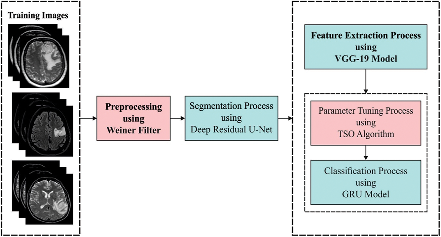
Figure 1: Overall process of ADRU-SCM method

2.1 WF Based Pre-Processing

The presented ADRU-SCM approach primarily applies WF based pre-processing to eradicate the noise that exists in it. Noise extraction is an image pre-processing technique where the feature of the image corrupted by noise, are heightened [16]. The adaptive filter is a certain instance where the denoising procedure totally relies on the noise contents i.e., existing in the image. Given that the corrupted image be a I^(x,y), the noise variance where the complete point is illustrated by σy2, the local mean is represented by μL^ about a pixel window and local variance from the window is implied by σ^y2. Next, the probable system of denoising the image is demonstrated by the following expression:

I^^=I^(x,y)−σy2σ^y2(I^(x,y)−μL^)(1)

Noe, the noise variance through the image becomes corresponding to zero, σy2=0=>I^^=I^(x,y). As soon as the global noise variance becomes lower whereas the local variance becomes larger when compared to global variance, the ratio is nearly equal to one.

When σ^y2≫σy2, I^^=I^(x,y). The superior local variance demonstrates the existence of edge from an image window. In such cases, when the local and global variance matches with one another, the equation is expressed by:

I^^=μL^ as σ^y2≈σy2(2)

2.2 Image Segmentation

The ADRU-SCM model follows deep residual U-Net segmentation model for determining the affected brain regions. By designing the U-Net model for image segmentation, the researchers used a DL algorithm U-Net with residual connection [17]. U-Net could also be improved by using residual units rather than plain units. By using residual connections, it maximizes the capability and the performance of the network. ResUnet incorporates the robustness of residual neural network and U-Net architecture. ResUnet has encompassed three major components, bridge, decoder, and encoder. In the encoder, the image served as an input is encoded to denser representations. The decoder part recovers the depiction to a pixel-wise classification. Such components are generated by residual units comprising two convolutional blocks using the size of 3×3 and an identity mapping connects the output and input units. The convolutional block contains a branch normalization (BN) layer and also it includes a convolutional layer and a Rectified linear unit activation (ReLU). The size of feature mappings is decreased by half with the stride of 2 in the convolutional block rather than applying pooling function in residual unit from the encoder to downsampling the feature mapping size. A convolution and sigmoid activation layers using a size of 1×1 are applied for projecting the multichannel map in the target segmentation following the last part of decoder. U-Net based residual unit semantic segmentation is chosen by the researcher since it functions with trained instances and provides more efficient outcomes for segmentation tasks. Furthermore, U-Net was mainly constructed for image segmentation.

2.3 VGG-19 Feature Extractor

VGG19 is a nineteen-layer difference of VGG method. It involves one SoftMax layer, 16 convolution layers, 3 FC layers, and 5 MaxPool layers [18]. Further, there are VGG versions namely VGG16, VGG11, etc. VGG19 has a computing capacity of 19.6 billion floating point operations for every second (FLOPs). In a convolutional neural network (CNN), there are three major layers: (i) pooling layer; (ii) fully-connected layer (FC); and (iii) convolutional layer. Once the FC layer is prepared for the last classification, they are trained by several pooling and convolution layers. CNN model that has been trained is utilized rather than a feature extractor. With the network that is previously trained as the feature extractor, the deeper CNN is performed by smaller datasets in other fields. This is due to the feature extractor having been trained previously. VGG19 network was trained for recognizing objects to make texture. When initiated DenseBox, they employed a pre-trained VGG19 architecture from ImageNet. DenseBox is an FCNN architecture for object recognition.

2.4 GRU Based Classification

Once the features are derived, the GRU approach was executed as a classification model. The most important shortcoming of traditional recurrent neural network (RNN) method is that once the time step increases, the network fails to derive the context from the time step of the prior state is termed long-term dependency [19]. Further, to resolve these problems, the long short term memory (LSTM) technique is determined by memory cells with multiple gates in hidden layer.

•   The ft forget gate selects that measure long-term state ct need to be neglected;

•   The it input gate control that measures of c~t should be additional to long-term form ct;

•   The gt output gate describes that amount of ct should be read and output to ht and ot.

The subsequent equation illustrates the long- and short-term procedures of cell and output of each layer in time step:

ft=σ(WxfT⋅xt+WhfT⋅ht−1+bf).(3)

it=σ(WxTi⋅xt+WhTi⋅ht−1+bi).(4)

ot=σ(WxTo⋅xt+WhTo⋅ht−1+bi).(5)

gt=tanh(WxTg⋅xt+WhTg⋅ht−1+bi).(6)

ct=ft⊗ct−1+it⊗c~t.(7)

ot,ht=gt⊗tanh(ct).(8)

From the expression, Whf,Whi,Who,Whg determines the weight matrix of the short-term form of previous time step, Wxf,Wxi,Wxo,Wxg indicates the weight matrix connecting input vector, and bf,bi,bo, and bg are bias. It is assumed that GRU has distinct implementations of transfer and collection of information that LSTM requires for employment.

rt=σ(WxrT⋅xt+WorT⋅ot−1+br).(9)

zt=σ(WxzT⋅xt+WoTz⋅ot−1+bz).(10)

o~t=tanh(Wxo~T⋅xt+Woo~T⋅(rt⊗ot−1)+bo~).(11)

ot=zt⊗ot−1+(1−zt)⊗ot.(12)

In the equation, Wxr,Wxz,Wxo~ refers to the weight matrix connecting input vector, Wor,Woz,Wo denotes the weight matrix of preceding time steps, and br,bz,bo~ are bias.

2.5 Hyperparameter Optimization

At the final stage, the TSO algorithm effectually tunes the GRU hyperparameters [20–22]. Kaur et al. [23] projected a bio-simulated optimized approach that simulates the natural foraging way of marine invertebrate, tunicate discharge bright bio luminescence. The numerical approach of jet propulsion was advanced from three limitations: residual nearby an optimum agent, prevent conflict amongst the exploration agent and followed the place of maximal qualified agent. Fig. 2 showcases the flowchart of TSO technique. In order to prevent inter agent conflicts if the seeking an optimum place, a novel agent place was evaluated as:

A→=G→M→(13)

G→=c2+c3−F→(14)

F→=c1⋅F→.(15)

In which A→ implies the vector of a new agent places, G→ denotes the gravity force, F→ stands for the water flow from the deep ocean, and c1, c2, and c3 signifies the three arbitrary amounts. The social force amongst the agents was stored from a new vector M→ is represented as:

M→=[Pmin+c1⋅Pmax−Pmin].(16)

At this point, Pmin=1 and Pmax=4 defines the 1st and 2nd sub-ordinates correspondingly signifying the speed of increasing social links. Following the project, optimum agents are essential for reaching optimal solutions. Therefore, to ensure that no conflict occurs amongst neighboring agents from the swarm, an optimum place of optimum agents is computed as:

PD→=|Xbest−rrand⋅Pp(x)→|(17)

In which PD→ stored the length amongst the optimal agents and food origin, Xbest denotes the optimum place, rrand indicates the stochastic value from the range of [0,1], and the vector Pp(x)→ is the place of tunicates at the time of iteration x. For ensuring that search agent is still nearby an optimum agent, their places were computed as:

Pp(x)→={ Xbest+A⋅P→D,if rrand≥0.5Xbest−A⋅P→D,if rrand<0.5 (18)

In which Pp(x)→ represents the upgrade places of agents at iteration x in comparison to optimum recorded place Xbest. In order to model the swarming performance of tunicates, the places of current agent are upgraded on the fundamental of the places of 2 agents:

Pp(x→+1)=Pp(x)→+Pp(x→+1)2+c1(19)

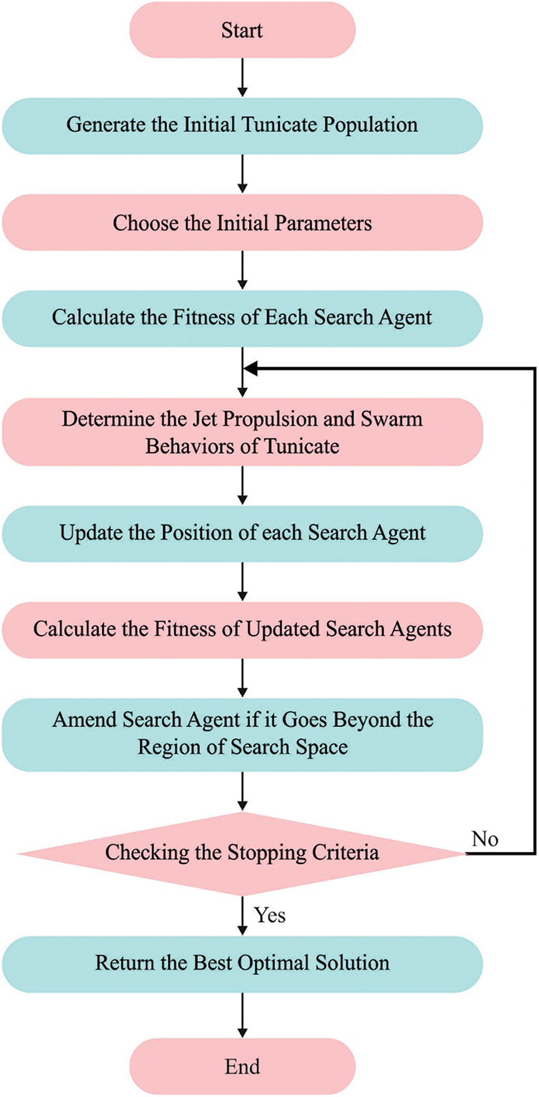
Figure 2: Flowchart of TSO technique

In order to clarify the TSO, important steps were given under to depict the flow of original TSO thoroughly [24].

1.    Initializing the primary population of tunicates P→p.

2.    Fixed the original value to parameter and the maximal count of iterations.

3.    Compute the fitness value of all the exploration agents.

4.    Next estimating the fitness, an optimum agent was inspected from the offered searching space.

5.    Upgrading the places of all the exploration agents in Eq. (19).

6.    Returning novel upgrade agents to their boundary.

7.    Compute the fitness cost of upgrade searching agents. If there is an optimum solution to preceding solutions, upgrade P→p and storing the optimum solution from Xbest.

8.    If the termination criteria were encountered, the processes end. Otherwise, iterate Steps 5–8.

9.    State the optimal solution (Xbest) which is reached so far.

The TSO system made a fitness function for achieving maximal classifier efficiency. It resolves a positive integer for representing best efficiency of candidate outcomes. During this case, the minimize of classify error rate was regarded as fitness function (FF) as provided in Eq. (20).

fitness(xi)=ClassifierErrorRate(xi)=number of misclassified samplesTotal number of samples∗100(20)

3  Results and Discussion

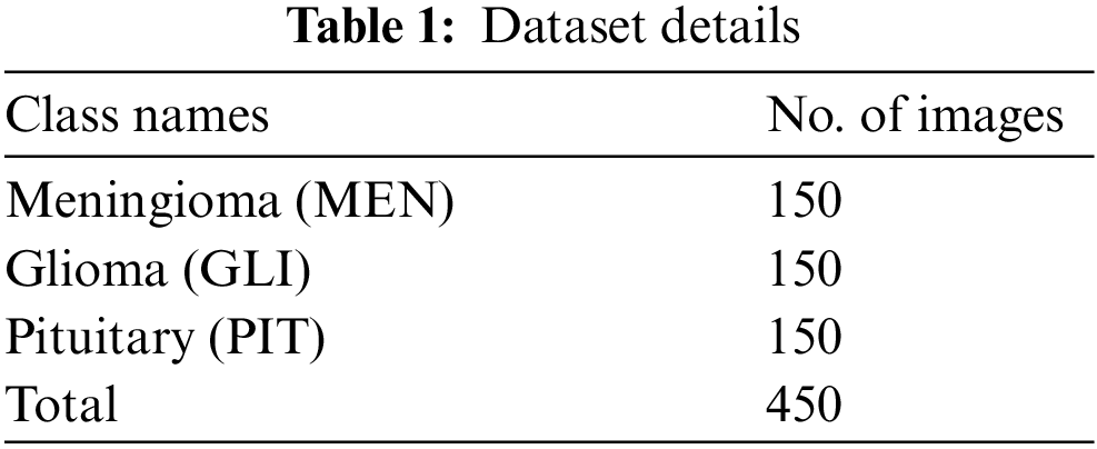
The performance validation of the ADRU-SCM techniques was tested with the help of Figshare dataset [25]. The dataset comprises 3 class labels with 150 images under Meningioma (MEN), 150 images under Glioma (GLI), and 150 images under Pituitary (PIT) classes as demonstrated in Tab. 1.

The set of confusion matrices created by the ADRU-SCM model under five distinct runs is given in Fig. 3. On run-1, the ADRU-SCM model has recognized 136 samples under MEN, 132 samples under GLI, and 146 samples under PIT class. Likewise, on run-3, the ADRU-SCM approach has identified 140 samples under MEN, 150 samples under GLI, and 143 samples under PIT class. Moreover, on run-5, the ADRU-SCM method has recognized 134 samples under MEN, 143 samples under GLI, and 143 samples under PIT class.

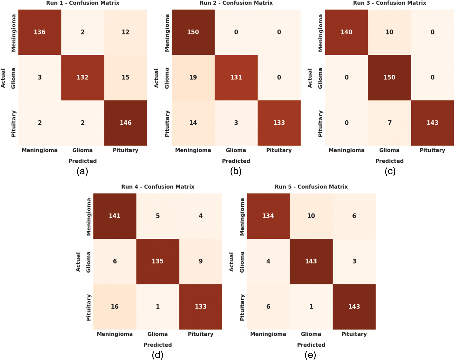
Figure 3: Confusion matrices of ADRU-SCM approach (a) Run1, (b) Run2, (c) Run3, (d) Run4, and (e) Run5

Tab. 2 offers overall classification outcomes of the ADRU-SCM methodology under five distinct runs. Fig. 4 portrays brief classifier results of the ADRU-SCM model under run-1. The figure inferred that the ADRU-SCM model has reached effectual classification performance under all classes. For sample, the ADRU-SCM model has classified samples under MEN class with accuy, sensy, specy, and Fscore of 95.78%, 90.67%, 98.33%, and 93.47% respectively. Also, the ADRU-SCM technique has classified samples under GLI class with accuy, sensy, specy, and Fscore of 95.11%, 88%, 98.67%, and 92.31% correspondingly. Besides, the ADRU-SCM approach has classified samples under PIT class with accuy, sensy, specy, and Fscore of 93.11%, 97.33%, 91%, and 90.40% correspondingly.

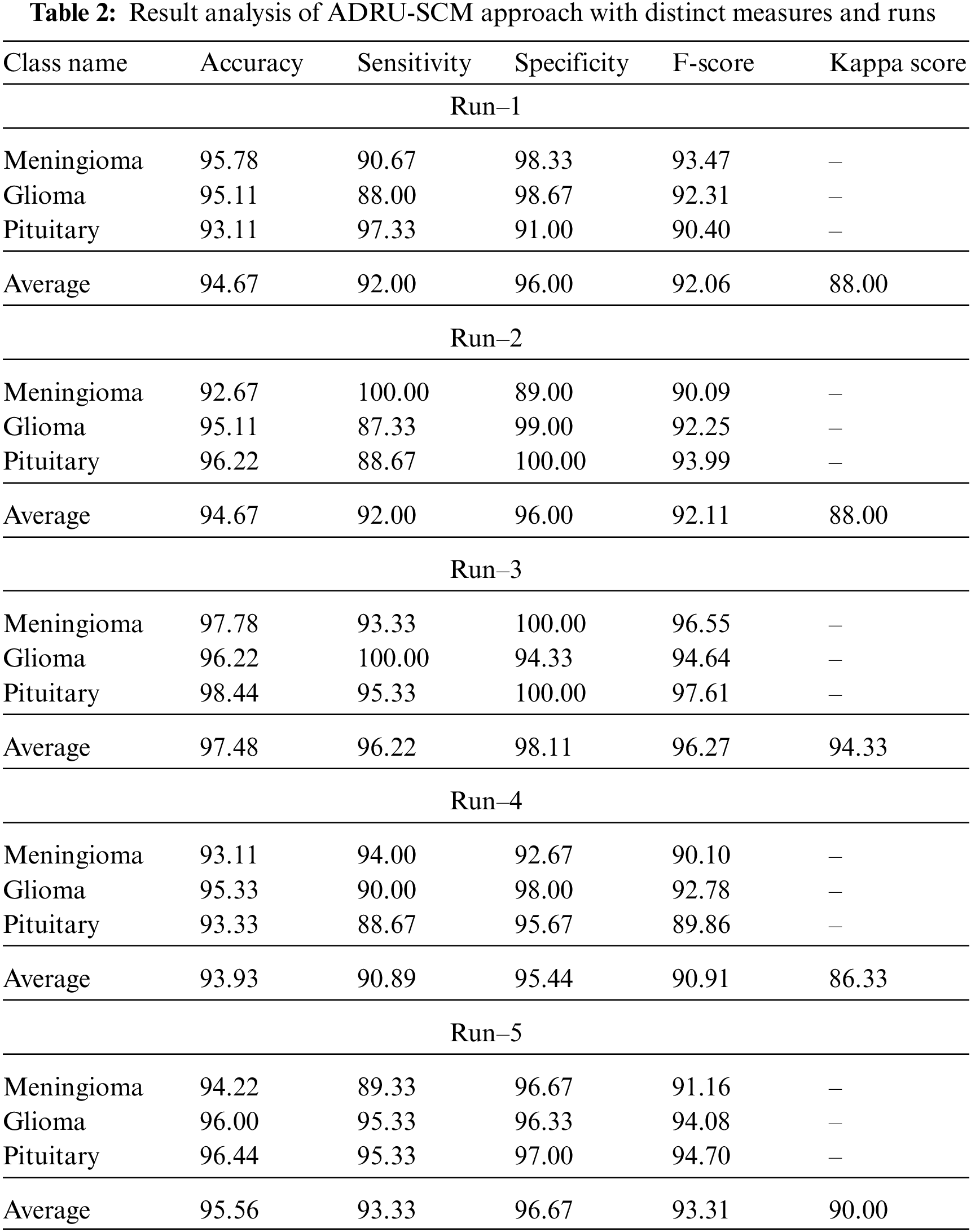
Figure 4: Average analysis of ADRU-SCM approach under Run-1

Fig. 5 depicts detailed classifier results of the ADRU-SCM methodology under run-2. The figure implied the ADRU-SCM system has reached effectual classification performance under all classes. For example, the ADRU-SCM approach has classified samples under MEN class with accuy, sensy, specy, and Fscore of 92.67%, 100%, 89%, and 90.09% correspondingly. Moreover, the ADRU-SCM method has classified samples under GLI class with accuy, sensy, specy, and Fscore of 95.11%, 87.33%, 99%, and 92.25% correspondingly. In addition, the ADRU-SCM approach has classified samples under PIT class with accuy, sensy, specy, and Fscore of 96.22%, 88.67%, 100%, and 993.99% correspondingly.

Figure 5: Average analysis of ADRU-SCM approach under Run-2

Fig. 6 represents brief classifier results of the ADRU-SCM approach under run-3. The figure inferred the ADRU-SCM algorithm has reached effectual classification performance under all classes. For example, the ADRU-SCM method has classified samples under MEN class with accuy, sensy, specy, and Fscore of 97.78%, 93.33%, 100%, and 96.55% respectively. Similarly, the ADRU-SCM methodology has classified samples under GLI class with accuy, sensy, specy, and Fscore of 96.22%, 100%, 94.33%, and 94.64% respectively. Also, the ADRU-SCM model has classified samples under PIT class with accuy, sensy, specy, and Fscore of 98.44%, 95.33%, 100%, and 97.61% correspondingly.

Figure 6: Average analysis of ADRU-SCM approach under Run-3

Fig. 7 shows brief classifier results of the ADRU-SCM method under run-4. The figure inferred that the ADRU-SCM methodology has reached effectual classification performance under all classes. For example, the ADRU-SCM system has classified samples under MEN class with accuy, sensy, specy, and Fscore of 93.11%, 94%, 92.67%, and 90.10% correspondingly. Along with that, the ADRU-SCM methodology has classified samples under GLI class with accuy, sensy, specy, and Fscore of 95.33%, 90%, 98%, and 92.78% correspondingly. Besides, the ADRU-SCM system has classified samples under PIT class with accuy, sensy, specy, and Fscore of 93.33%, 88.67%, 95.67%, and 89.86% correspondingly.

Figure 7: Average analysis of ADRU-SCM approach under Run-4

Fig. 8 reveals detailed classifier results of the ADRU-SCM method under run-5. The figure implied the ADRU-SCM system has reached effectual classification performance under all classes. For example, the ADRU-SCM methodology has classified samples under MEN class with accuy, sensy, specy, and Fscore of 94.22%, 89.33%, 96.67%, and 91.16% correspondingly. Moreover, the ADRU-SCM technique has classified samples under GLI class with accuy, sensy, specy, and Fscore of 96%, 95.33%, 96.33%, and 94.08% correspondingly. Also, the ADRU-SCM system has classified samples under PIT class with accuy, sensy, specy, and Fscore of 96.44%, 95.33%, 97%, and 94.70% correspondingly.

Figure 8: Average analysis of ADRU-SCM approach under Run-5

The training accuracy (TA) and validation accuracy (VA) obtained by the ADRU-SCM method on phishing email classification is illustrated in Fig. 9. The experimental outcome inferred that the ADRU-SCM technique has reached maximum values of TA and VA. Particularly, the VA is higher than TA.

Figure 9: TA and VA analysis of ADRU-SCM methodology

The training loss (TL) and validation loss (VL) gained by the ADRU-SCM approach to phishing email classification are established in Fig. 10. The experimental outcome implied the ADRU-SCM method has accomplished least values of TL and VL. Specifically, the VL seemed to be lower than TL.

Figure 10: TL and VL analysis of ADRU-SCM methodology

At last, a brief comparative analysis of the ADRU-SCM approach with existing DL models is performed in Tab. 3 [26]. Fig. 11 highlights the comparative accuy investigation of the ADRU-SCM method with existing models. The figure indicated that the MobileNetV2 approach has shown ineffective outcomes with least accuy of 92.78%. Similarly, the Inception v3 and ResNet50 models have obtained slightly increased accuy of 93.34% and 93.10% respectively. Though the hybrid gravitational search optimization (HGSO) and DenseNet201 models have resulted in reasonable accuy of 96.66% and 94.63%, the ADRU-SCM model has shown effectual outcomes with higher accuy of 97.84%.

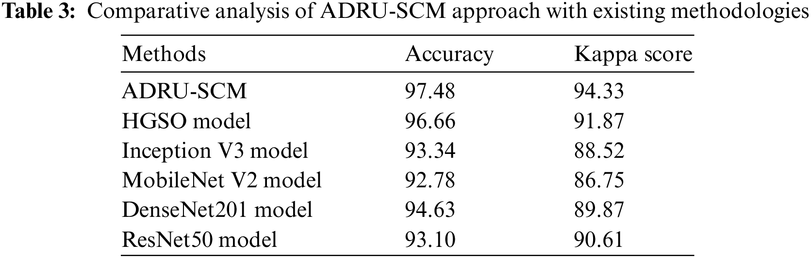
Figure 11: Accuy analysis of ADRU-SCM method with existing algorithms

Fig. 12 highlights the comparative kappa examination of the ADRU-SCM method with recent models. The figure denoted the MobileNetV2 technique has shown an ineffective outcome with least kappa of 86.75%. Meanwhile, the Inception v3 and ResNet50 techniques have gained slightly increased kappa of 88.52% and 86.75% correspondingly. Though the HGSO and DenseNet201 approaches have resulted in reasonable kappa of 91.87% and 89.87%, the ADRU-SCM system has shown effectual outcome with higher kappa of 94.33%.

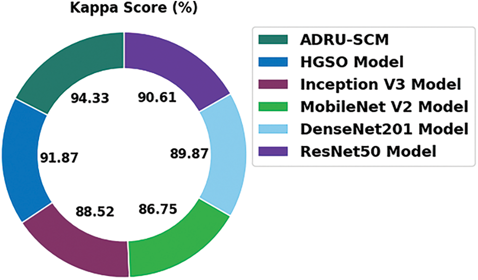
Figure 12: Kappa analysis of ADRU-SCM approach with existing algorithms

These results and discussion clearly pointed out the better performance of the ADRU-SCM model over recent approaches.

4  Conclusion

In this study, a novel ADRU-SCM model was established for the segmentation and classification of BT. The presented ADRU-SCM approach initially applies WF based pre-processing to eradicate the noise that exists in it. In addition, the ADRU-SCM model follows deep residual U-Net segmentation model to determine the affected brain regions. Moreover, VGG-19 model is exploited as a feature extractor. Finally, TSO with GRU model is applied as a classification model and the TSO algorithm effectually tunes the GRU hyperparameters. The performance validation of the ADRU-SCM model was tested utilizing FigShare dataset and the results pointed out the better performance of the ADRU-SCM model over recent approaches. Thus, the ADRU-SCM model can be applied to carry out BT classification procedure. In future, the performance of ADRU-SCM approach is enhanced by the use of metaheuristic based deep instance segmentation models.

Funding Statement: This work was supported by the 2022 Yeungnam University Research Grant.

Conflicts of Interest: The authors declare that they have no conflicts of interest to report regarding the present study.

References

 1.  A. Tiwari, S. Srivastava and M. Pant, “Brain tumor segmentation and classification from magnetic resonance images: Review of selected methods from 2014 to 2019,” Pattern Recognition Letters, vol. 131, no. 9, pp. 244–260, 2020. [Google Scholar]

 2.  G. Neelima, D. R. Chigurukota, B. Maram and B. Girirajan, “Optimal DeepMRSeg based tumor segmentation with GAN for brain tumor classification,” Biomedical Signal Processing and Control, vol. 74, no. 1, pp. 103537, 2022. [Google Scholar]

 3.  K. Kumar and R. Boda, “A multi-objective randomly updated beetle swarm and multi-verse optimization for brain tumor segmentation and classification,” The Computer Journal, vol. 65, no. 4, pp. 1029–1052, 2021. [Google Scholar]

 4.  B. Tahir, S. Iqbal, M. U. G. Khan, T. Saba, Z. Mehmood et al., “Feature enhancement framework for brain tumor segmentation and classification,” Microscopy Research and Technique, vol. 82, no. 6, pp. 803–811, 2019. [Google Scholar]

 5.  E. S. Biratu, F. Schwenker, Y. M. Ayano and T. G. Debelee, “A survey of brain tumor segmentation and classification algorithms,” Journal of Imaging, vol. 7, no. 9, pp. 179, 2021. [Google Scholar]

 6.  J. Amin, M. Sharif, M. Yasmin, T. Saba, M. A. Anjum et al., “A new approach for brain tumor segmentation and classification based on score level fusion using transfer learning,” Journal of Medical Systems, vol. 43, no. 11, pp. 326, 2019. [Google Scholar]

 7.  M. Sharif, U. Tanvir, E. U. Munir, M. A. Khan and M. Yasmin, “Brain tumor segmentation and classification by improved binomial thresholding and multi-features selection,” Journal of Ambient Intelligence and Humanized Computing, vol. 219, no. 1, pp. 1–20, 2018. http://dx.doi.org/10.1007/s12652-018-1075-x. [Google Scholar]

 8.  M. Y. B. Murthy, A. Koteswararao and M. S. Babu, “Adaptive fuzzy deformable fusion and optimized CNN with ensemble classification for automated brain tumor diagnosis,” Biomedical Engineering Letters, vol. 12, no. 1, pp. 37–58, 2022. [Google Scholar]

 9.  S. Dasanayaka, S. Silva, V. Shantha, D. Meedeniya and T. Ambegoda, “Interpretable machine learning for brain tumor analysis using MRI,” in 2022 2nd Int. Conf. on Advanced Research in Computing (ICARC), Belihuloya, Sri Lanka, pp. 212–217, 2022. [Google Scholar]

10. S. Krishnakumar and K. Manivannan, “Effective segmentation and classification of brain tumor using rough K means algorithm and multi kernel SVM in MR images,” Journal of Ambient Intelligence and Humanized Computing, vol. 12, no. 6, pp. 6751–6760, 2020. [Google Scholar]

11. A. Ilhan, B. Sekeroglu and R. Abiyev, “Brain tumor segmentation in MRI images using nonparametric localization and enhancement methods with U-net,” International Journal of Computer Assisted Radiology and Surgery, vol. 17, no. 3, pp. 589–600, 2022. [Google Scholar]

12. A. R. Raju, P. Suresh and R. R. Rao, “Bayesian HCS-based multi-SVNN: A classification approach for brain tumor segmentation and classification using bayesian fuzzy clustering,” Biocybernetics and Biomedical Engineering, vol. 38, no. 3, pp. 646–660, 2018. [Google Scholar]

13. S. Das, G. Nayak, L. Saba, M. Kalra, J. Suri et al., “An artificial intelligence framework and its bias for brain tumor segmentation: A narrative review,” Computers in Biology and Medicine, vol. 143, no. 3, pp. 105273, 2022. [Google Scholar]

14. D. Kapila and N. Bhagat, “Efficient feature selection technique for brain tumor classification utilizing hybrid fruit fly based ABC and ANN algorithm,” Materials Today: Proceedings, vol. 51, pp. 12–20, 2022. [Google Scholar]

15. B. Song, C. R. Chou, X. Chen, A. Huang and M. C. Liu, “Anatomy-guided brain tumor segmentation and classification,” in Int. Workshop on Brainlesion: Glioma, Multiple Sclerosis, Stroke and Traumatic Brain Injuries, BrainLes 2016: Brainlesion: Glioma, Multiple Sclerosis, Stroke and Traumatic Brain Injuries, Lecture Notes in Computer Science Book Series, Athens, Greece, vol. 10154, pp. 162–170, 2016. [Google Scholar]

16. K. Shankar, M. Elhoseny, S. K. Lakshmanaprabu, M. Ilayaraja, R. M. Vidhyavathi et al., “Optimal feature level fusion based ANFIS classifier for brain MRI image classification,” Concurrency and Computation: Practice and Experience, vol. 32, no. 1, pp. 1–12, 2020. [Google Scholar]

17. M. Z. Alom, C. Yakopcic, M. Hasan, T. M. Taha and V. K. Asari, “Recurrent residual U-Net for medical image segmentation,” Journal of Medical Imaging, vol. 6, no. 1, pp. 1, 2019. [Google Scholar]

18. D. Bhowmik, M. Abdullah, R. Bin and M. T. Islam, “A deep face-mask detection model using DenseNet169 and image processing techniques,” Doctoral dissertation, Brac University, 2022. [Google Scholar]

19. H. M. Lynn, S. B. Pan and P. Kim, “A deep bidirectional GRU network model for biometric electrocardiogram classification based on recurrent neural networks,” IEEE Access, vol. 7, pp. 145395–145405, 2019. [Google Scholar]

20. R. Sowmyalakshmi, T. Jayasankar, V. A. PiIllai, K. Subramaniyan, I. V. Pustokhina et al., “An optimal classification model for rice plant disease detection,” Computers, Materials & Continua, vol. 68, no. 2, pp. 1751–1767, 2021. [Google Scholar]

21. D. N. Le, V. S. Parvathy, D. Gupta, A. Khanna, J. J. P. C. Rodrigues et al., “IoT enabled depthwise separable convolution neural network with deep support vector machine for COVID-19 diagnosis and classification,” International Journal of Machine Learning and Cybernetics, vol. 12, no. 11, pp. 3235–3248, 2021. [Google Scholar]

22. D. Venugopal, T. Jayasankar, M. Y. Sikkandar, M. I. Waly, I. V. Pustokhina et al., “A novel deep neural network for intracranial haemorrhage detection and classification,” Computers, Materials & Continua, vol. 68, no. 3, pp. 2877–2893, 2021. [Google Scholar]

23. S. Kaur, L. K. Awasthi, A. L. Sangal and G. Dhiman, “Tunicate Swarm Algorithm: A new bio-inspired based metaheuristic paradigm for global optimization,” Engineering Applications of Artificial Intelligence, vol. 90, no. 2, pp. 103541, 2020. [Google Scholar]

24. F. N. Al-Wesabi, M. Obayya, A. M. Hilal, O. Castillo, D. Gupta et al., “Multi-objective quantum tunicate swarm optimization with deep learning model for intelligent dystrophinopathies diagnosis,” Soft Computing, vol. 318, no. 3, pp. 2199, 2022. http://dx.doi.org/10.1007/s00500-021-06620-5. [Google Scholar]

25. J. Cheng, “Brain tumor dataset,” Figshare, 2017. [Online]. Available: http://dx.doi.org/10.6084/m9.figshare.1512427.v5. [Google Scholar]

26. T. Sadad, A. Rehman, A. Munir, T. Saba, U. Tariq et al., “Brain tumor detection and multi-classification using advanced deep learning techniques,” Microscopy Research and Technique, vol. 84, no. 6, pp. 1296–1308, 2021. [Google Scholar]