Feature Fusion-Based Deep Learning Network to Recognize Table Tennis Actions

1  Introduction

Motion capture systems can effectively detect human movements. Motion capture systems based on inertial sensors have been used in various studies because their small size, low cost, and adaptability to different environments enable them to be integrated with wearable devices for the monitoring and recording of body movement [1]. Athletes have used wearable devices to monitor their training and movements to improve their fitness and performance [2–4]. Scientific training methods and equipment are highly valued in athletics. Conventional training equipment and methods that lack theoretical basis have been gradually replaced or improved by new methods through continual testing and by accumulating training experience. Thus, wearable devices are widely used in studies of various human activities [5–7].

In sports competitions, particularly individual sports, motion analysis is advantageous for athletes because the results can provide them with useful feedback on performance; this feedback can be used to improve performance with corrective exercises. Experiments on applications of motion analysis in sports are becoming more common. For example, Malawski studied motion in fencing by placing two nine-axis sensors on the elbow and chest of athletes to collect data. They then used a linear support vector machine to analyze fencing accuracy and fencing footwork [8]. In rowing, Worsey et al. reviewed various related studies and noted that most researchers placed sensors on rowing equipment to monitor rowing performance [9]. In swimming, Guignard et al. placed two nine-axis sensors on the upper and lower arms of swimmers to analyze swimming performance [10]. In running, Struber et al. used an S-Move system consisting of five nine-axis sensors to achieve three-dimensional automatic and dynamic gait analysis [11]. In table tennis, Tabrizi et al. developed a forehand stroke evaluation system with a single nine-axis sensor to provide players, particularly new players, actual practice with three forehand strokes [12].

Although wearable devices are widely used in data collection for various human actions, the positioning of the devices on the body must be related to the action being studied; otherwise, the accuracy of action recognition will be reduced. Placing sensors in optimal positions is key for action recognition [13,14]. Therefore, some studies on wearable devices have used multiple sensors to improve accuracy. However, placing multiple sensors on different parts of the body can be difficult, inhibiting, or uncomfortable for research participants [15]. The number of sensors must also be considered for motion capture in some sports. Studies have analyzed and predicted physical activities through appropriate experiments. Therefore, to obtain optimal table tennis data for subsequent activity analysis and estimation, this study referred to studies of racket sports, such as badminton and table tennis, in [16,17]. In these studies, different accelerometer, gyroscope, or magnetometer placements on the body may affect action recognition accuracy. According to the results of [16] and [17], a single sensor had the highest accuracy when worn on the wrist. Therefore, a single sensor was placed on the wrists of the participants for data collection in this study.

Artificial intelligence techniques have also matured in recent years. Some studies have combined wearable devices with artificial intelligence to achieve more accurate action recognition. Lawal et al. used accelerometers and gyroscopes to measure motion for seven different parts of the human body and applied a dual-channel convolutional neural network (CNN) for data classification. The CNN was able to obtain an F1 score of 90% on a public database. The results revealed that using complementary data from both accelerometers and gyroscopes for different body parts enabled the system to effectively classify actions, and data from sensors on the neck and the waist had a greater effect on action recognition accuracy [18]. Gholamiangonabadi et al. proposed a leave-one-subject-out cross-validation network architecture. The network comprised six feedforward neural networks and CNNs, and 10-fold cross validation was used for human action recognition. The accuracy reached 99.85% [19]. Tufek et al. used ZigBee modules to automatically collect human action data. Due to the imbalanced data in the data set, they used data augmentation to improve the performance. The last three layers of the long short-term memory (LSTM) network they used had the highest accuracy of 93% [20]. Büthe et al. placed a single sensor on a tennis racket and had two sensors attached to player’s shoes to capture data related to arm movements and footwork during a shot. A longest common subsequence algorithm was used, and five shots and three footwork patterns were recognized, and accuracy of shot and footwork recognition was 94% and 95%, respectively [21]. Brzostowski et al. used a Pebble smartwatch to collect acceleration data and used mel-frequency cepstral coefficients for feature extraction. Subsequently, principal component analysis was used to reduce the dimensionality of the data, and finally k-nearest neighbors and logistic regression models were employed to perform 10-fold cross validation on tennis shots. The accuracy of the k-nearest neighbors and logistic regression models were 82.22% and 87.99%, respectively, whereas the accuracy of the leave-one-out cross validation was 82.16% and 87.16%, respectively [22]. Pei et al. used a six-axis sensor for data collection and trained a model with a 50% overlapping register window and gravity, and the model achieved 98% accuracy for shot detection. It achieved 96% accuracy for three types of shot recognition and 80% accuracy for two types of spin recognition [23]. Pardo et al. placed six-axis sensors on participant wrists and waists for data collection and used a CNN to classify four shots in tennis and seven non-tennis activities with a mean accuracy of 99% [24]. Yen et al. used deep learning with feature fusion method into wearable sensor devices for human activity recognition and the accuracies in tenfold cross-validation were 99.56% and 97.46%, respectively [25].

Different deep learning networks are suitable for application in different fields. To determine the suitable deep learning network for action recognition, certain studies have used multiple networks for testing. Sansan et al. analyzed deep learning networks suitable for activity recognition and compared their performance in terms of accuracy, speed, and memory. Deep learning networks such as CNN, LSTM, bidirectional LSTM, gated recurrent unit, and deep belief networks were compared, and 10 groups of public databases were analyzed. Each dataset included acceleration and angular velocity data for different body parts. The analysis results for various networks revealed that CNN was effective for capturing activity signals and identifying correlations between sensors. In most cases, it had excellent performance with faster response speed and lower memory consumption than other networks. Sun et al. used multi-feature learning model with enhanced local attention and lightweight feature optimized CNN with joint learning strategy for vehicle re-identification [26,27]. In summary, wearable sensors have been widely used to classify actions, and sensor positioning has a substantial effect on the accuracy of action recognition. To accurately recognize the four table tennis strokes (i.e., forehand, backhand, forehand cut, and backhand cut), the sensors were placed on the back of the hands of the participants. Several tests revealed that hand movements had a greater correlation with the data collected for strokes. Thus, acceleration and angular velocity data of the hand measured by an accelerometer and gyroscope, respectively, can be used in an artificial neural network for action recognition.

The rest of this study is organized as follows. Section 2 describes the hardware architecture of the wearable device, data recording conditions, sensor calibration methods, and distribution of the recorded database data in the training, validation, and test sets. Section 3 explains the motion signal acquisition, data measurement method, input format, and network architecture. Section 4 introduces the calculation methods for evaluation metrics and accuracy used in the experiment. Section 5 presents the experimental results for different convolutional networks and discusses the evaluation results. Finally, Section 6 is the conclusion.

2  Experimental Setup

2.1 Hardware Architecture

The wearable device used in this study comprised a Raspberry Pi 3, a six-axis sensor (MPU-6050), and a power bank with a capacity of 10050 mAh. Because the power bank must provide power to the Raspberry Pi 3 for a long time during data measurement, its large volume and weight may affect participant performance. Therefore, the power bank was tied to the waist, the Raspberry Pi 3 was fixed on the arm, and the six-axis sensor was installed on the back of the hand to collect the acceleration and angular velocity values of different strokes as input data for the deep learning network proposed in this study. Because there are two types of billiard rackets, and the grips of the two types are different. In order to avoid different grips affecting the calibration of the sensor, we placed the sensor on the handle to avoid inconsistencies in the sensing data. The placement of the wearable device is presented in Fig. 1.

Figure 1: Placement of the wearable device

In this experiment, the Raspberry Pi 3 was used as a microcontroller for data acquisition, and an inter-integrated circuit communication protocol was used to obtain movement signals measured by the six-axis sensor. Angular velocity on the hand can be measured in ±250 °/s, ±500 °/s, ±1000 °/s, and ±2000 °/s. Acceleration measurement range and recall were ±16 g and 2048 LSB/g, respectively, and the gyroscope was set to ±2000 °/s and 16.4 LSB/(°/s). The output signals of the accelerometer and gyroscope were sampled at a frequency of 10 Hz, and the power bank was DC 5 V at 2.1 A and provided stable power for the wearable device.

2.2 Database of Recorded Experimental Data

To enhance the stability of our 6-axis sensor. Before wearing the device, the six-axis sensor was first calibrated by collecting 1000 data and taking the mean as to determine error during calibration. The x-, y-and z-axes of the gyroscope were calibrated simultaneously. Because the x-, y-and z-axes of the accelerometer were calibrated using gravity, their calibration was performed separately. The direction and position of the six-axis sensor were strictly controlled. The x-axis was toward the fingertip, the y-axis was toward the left side of the back of the hand, and the z-axis was toward the palm, as displayed in Fig. 2.

During the experiment, the wearable device was used to collect data in accordance with this specification. During data collection, the sensor must be worn in a fixed position and orientation. A loose sensor may affect overall data recording during movement, resulting in reduced accuracy. Therefore, the hand was wrapped with a wrist guard, and the six-axis sensor was placed on top of it. The wrist guard was used to fix the wearable device on the back of the hand without shaking, and effectively reduced the error in the collected data.

Figure 2: Six-axis sensor on the back of the hand

In this study, 20 participants were recruited to use their right hands to perform four basic table tennis strokes: forehand, backhand, forehand cut, and backhand cut. In order to avoid the participants data being too monotonous, each experimenter performed 4 different billiard actions 600 times. The Raspberry Pi 3 was used to collect data from the six-axis sensor at a rate of 10 Hz, and the data were stored in a text file. A total of 2400 values were recorded in the database as a 30 × 60 matrix with 60 eigenvalues. The collected data were divided into training (80%), validation (10%), and test sets (10%). The number of each type of stroke recorded in each data set is listed in Tab. 1.

3  Algorithm for Table Tennis Stroke Recognition

Stroke recognition was performed with data collection and the subsequent use of a deep learning algorithm to recognize different strokes. The details of the proposed action recognition algorithm are described in the following section.

3.1 Motion Signal Acquisition

A wearable device was used to measure the experimental data for acceleration and angular velocity of the participant’s hand while performing a stroke. The participants performed four table tennis strokes: forehand, backhand, forehand cut, and backhand cut. Fig. 3 presents plots of acceleration and angular velocity values vs. time during the stroke.

Figure 3: Line graphs for acceleration (left) and angular velocity (right) during a single swing: (a) fore hand; (b) back hand; (c) fore hand cut; (d) back hand cut

3.2 Data Measurement Methods and Formats

During data collection, the data of the participants were collected at one stroke per second, and the sensor collected six values for acceleration (x, y, and z-axes) and angular velocity (x, y, and z-axes) at a sampling frequency of 10 Hz; thus, a 1×60 matrix was stored each second. The matrix was recorded in the following order: x-axis acceleration, y-axis acceleration, z-axis acceleration, x-axis angular velocity, y-axis angular velocity, and z-axis angular velocity. Data were collected for 30 s; thus, a 30×60 matrix was stored for each measurement.

3.3 Network Architecture

A CNN was used in this study because it can extract input signal features through its convolutional layer, eliminating the need for manual feature extraction in conventional machine learning. Furthermore, the CNN can learn and classify through its fully connected layers. In this study, multiscale CNN was used for feature fusion, and multiscale correlation features of different lengths were obtained through kernels of different sizes [28] to achieve feature extraction at different scales.

The six-axis sensor signals collected by the wearable device were first stored in a fixed format before normalization. Values were normalized as in Eq. (1). The minimum value min(xi) in the number sequence was subtracted from the initial value xi, and the difference was divided by the difference between the maximum value max(xi) of the sequence and the minimum value min(xi) of the sequence. The result x~i was scaled in the range of 0 to 1.

x~i=xi−min(xi)max(xi)−min(xi)(1)

where, xi is the input data.

To enable the CNN to predict the correct action with data from a single stroke, the 1×60 data of one stroke were normalized and were used as input to the proposed network architecture. Among these, convolution blocks with three different kernel sizes, A, B, and C, were used for primary feature extraction. Features of different scales were input to the fully connected layers for learning and classification through subsequent concatenation, as presented in Fig. 4.

Figure 4: CNN architecture combining three different feature extraction methods

Convolutional blocks A and B were concatenated as the input for the next layer of network. The subsequent network comprised two sets of fully connected layers, and the fully connected layers were used for feature classification. The maximum pooling layer, batch normalization, and random dropout between each convolutional layer were used in the convolutional blocks. The maximum pooling layer was used to retain only the most influential features, whereas batch normalization was used to normalize the data to values between 0 and 1. The maximum pooling layer and batch normalization were used to reduce computations during network training and to increase the speed of the network; random dropout was used to prevent overfitting during network training. The activation function used a rectified linear unit to enable the network to calculate nonlinear problems. The rectified linear unit converts the output of some neurons to 0 to reduce overfitting. In the final computation, the Softmax function was used to calculate the probability of each of the four strokes, and the stroke with the highest probability was selected as the classification result. The overall network architecture is presented in Fig. 4. Groups of 60 values collected with the accelerometer and gyroscope were used as input data for training the CNN; each group of values was the data collected for one stroke. The data was processed with the convolutional blocks of A and B for feature extraction, and then passed through two fully connected layers with 256 and 128 neurons, respectively, to obtain one of the final four possible outputs of forehand, backhand, forehand cut, and backhand cut. The convolutional blocks A and B are presented in Fig. 5.

Figure 5: Network architecture of the convolutional blocks of different scales: (a) A; (b) B

The three convolutional layers comprised 32, 64 and 128 neurons, respectively, and the stride was set to 1. The kernel size was set to 3 in block A and 5 in block B; otherwise, the blocks were identical. Masking of the max pooling layer was performed with a 1 × 3 matrix, the stride was set to 2, and the random dropout was set to 0.25. The Adam optimizer was used in this study with a learning rate of 0.001; this learning rate decreased by 10% after every 10 iterations. The loss function used categorical cross-entropy to calculate errors between predicted and actual values to adjust the training weights of the model, and the number of iterations of the CNN was set to 200.

4  Calculation Methods of Evaluation Metrics and Accuracy

Solutions to classification problems in deep learning or statistics can be evaluated using a confusion matrix. The rows of the confusion matrix are the actual classes, the columns are the predicted classes, and the results are presented as the number of predictions for each actual–predicted class pairing. As presented in Tab. 2, true positive (TP) indicates that the actual value is positive and the predicted value is also positive; false negative (FN) means that the actual value is positive and the predicted value is negative; false positive (FP) indicates that the actual value is negative and the predicted value is positive; and true negative (TN) means that the actual value is negative and the predicted value is also negative.

Network prediction aims to have high accuracy. Values in the confusion matrix are number counts and may be difficult to use to evaluate the quality of a model directly for large amounts of data. Therefore, four metrics of accuracy, precision, recall, and specificity were calculated using TP, FN, FP, and TN.

Accuracy: The proportion of the correct prediction results to all predictions. In this study, the accuracy is the proportion of strokes that were correctly predicted, and it can be calculated with Eq. (2).

Accuracy=TP+TNTP+TN+FP+FN(2)

Precision: For a single-class item, TP indicates the proportion of positive predictions. For example, if forehand is considered positive and the other actions are considered negative, precision can be calculated by dividing the number of correctly classified forehands by the total number of predicted forehands (both correctly and incorrectly classified). High precision indicates a high probability of correctly predicting an outcome. Precision can be calculated as in Eq. (3).

Precision=TPTP+FP(3)

Recall: As for precision, if forehand is positive and other actions are negative, recall is the number of correctly classified forehands divided by the sum of the number of correctly classified forehands and the number of incorrectly classified non-forehand strokes. That is, recall is the number of correctly recognized swings of all recognized swings. A high recall indicates a high probability of returning most relevant results, and recall can be calculated with Eq. (4).

sensitivity=Recall=TPTP+FN(4)

Specificity: For a single-class item, TN is the proportion of the actual negative classifications. Again assuming that forehand is positive and other actions are negative, specificity is the number of correctly classified actions divided by the number of correctly classified other actions plus the number of incorrectly classified forehands. That is, specificity is the number of all other actions that were correctly recognized. High specificity indicates a high probability of correctly recognizing all other actions. Specificity can be calculated with Eq. (5).

Specificity=TNTN+FP(5)

These four metrics can be used to convert confusion matrix values onto an interval of 0 to 1, and another indicator, the F1 score, can be generated.

F1 score is the harmonic mean of precision and recall. The score measures improvements in precision and recall while minimizing their difference. Its value falls between 0 and 1; 1 represents the optimal output of the model, and 0 represents random output. The F1 score is calculated with Eq. (6).

F1Score=2∗Precision∗RecallPrecision+Recall(6)

Binary classification was performed four times on each of the four classes to calculate the accuracy, precision, recall, specificity and F1 score for each of the four table tennis strokes. The mean values were used as metrics to evaluate the model.

The CNN was also evaluated by k-fold cross validation. The k-fold cross validation method is used to reduce errors in the actual values due to specific combinations of training and testing data. In k-fold cross validation, raw data are classified into k groups, and a nonrepeated group was selected as the test set for each run. The remaining k−1 unselected groups were used as the training set. Training was repeated k times to obtain k accuracy values. In this study, k was set as 5, as in Fig. 6. The accuracies of the five trials were averaged as the overall model accuracy.

Figure 6: Five-fold cross validation

5  Experimental Results and Discussion

5.1 Evaluation Metrics of the Models

Each participant performed four types of table tennis strokes in the experimental environment. The CNN models were trained with the collected data. Five models were trained, four of which were conventional CNNs, and one was a multiscale CNN. The evaluation results after model training are presented in Tab. 3, with Kernel Size_1, Kernel Size_3, Kernel Size_5, and Kernel Size_7 all being conventional CNNs with kernel sizes of 1, 3, 5, and 7, respectively. The final F1 score results revealed that the convolution layer could effectively identify features that improved the training and predictions of the model for kernel sizes of 3 and 5. To further improve the model, a multiscale CNN model combining the features of Kernel Size_3 and Kernel Size_5 was used. The results in Tab. 3 revealed that the multiscale CNN model had an accuracy, precision, recall, specificity, and F1 score of 99.58%, 99.16%, 99.19%, 99.72%, and 99.16%, respectively; the multiscale model outperformed the conventional CNN models in all metrics.

5.2 Confusion Matrix of the Models

Fig. 7 presents the confusion matrices for all models. The results revealed that the Kernel Size_3 and Kernel Size_5 models could accurately recognize the forehand and backhand. The multiscale CNN model also recognized these actions but had improved recognition accuracy for forehand cut and backhand cut. Thus, the feature fusion technique can effectively improve predictions of table tennis strokes.

Figure 7: Confusion matrix for different CNN models: (a) Kernel size_1 (b) Kernel size_3 (c) Kernel size_5 (d) Kernel size_7 (e) Multi-scale

5.3 Accuracy and Loss Function of the Models

Figs. 8 to 12 present the accuracy and loss function curves for all trained models. These curves reveal the convergence of model and judge whether the model was stable during training. Blue and orange lines in the graphs represent the training and validation results, respectively. Figs. 8 to 11 present the accuracy and loss function curves of the conventional CNN models. The figures reveal that the models could not achieve stable convergence even after 200 iterations and had slight oscillations. Fig. 12 presents the multiscale CNN model; the model began to converge at 100 iterations and fully converged after 160 iterations. The full 200 iterations were not executed because an early stopping mechanism was used to avoid overtraining and overfitting.

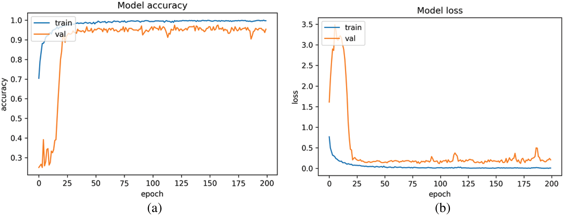
Figure 8: Kernel size_1 model: (a) Accuracy curve; (b) Loss function curve

Figure 9: Kernel size_3 model: (a) Accuracy curve; (b) Loss function curve

Figure 10: Kernel size_5 model: (a) Accuracy curve; (b) Loss function curve

Figure 11: Kernel size_7 model: (a) Accuracy curve; (b) Loss function curve

Figure 12: Multiscale model: (a) Accuracy curve; (b) Loss function curve

5.4 Cross Validation Results of the Models

Network training is a probabilistic model, and the combination of a set of data sets cannot prove that the results are representative of the network. To prevent the prediction results by being affected by fixed training and testing data, five-fold cross validation was adopted to evaluate the results. The five-fold cross validation results in Tab. 4 were consistent with the previous results. The multiscale CNN model had an accuracy of 99.87% and an error of ± 0.17% in action recognition; thus, it could more accurately recognize table tennis strokes than conventional CNN models could. This result also shows that the multi-scale convolutional neural network has better robustness after five-fold cross validation.

6  Conclusions

Professional sports teams or amateur sports enthusiasts have recognized the potential of technology and data analysis; they have thus begun to use wearable devices to collect data related to physical activities. These wearables generate large amounts of data for research and analysis to determine whether an athlete has correct posture and stroke during sports and to identify more effective training methods to improve athlete performance.

This study proposed a system for classifying table tennis strokes. In the system, a wearable device containing a six-axis sensor was tied on the back of the hand to collect data during racket movements. Features of the six-axis sensor were determined using a CNN with two different kernel sizes, and actions were classified with the CNN models. Besides, the early stopping mechanism was used to avoid overtraining and overfitting conditions. The accuracy after five-fold cross validation reached 99.87%, demonstrating that the new CNN (multiscale CNN) used in this study was more effective than conventional CNNs in action recognition.

Acknowledgement: We thanks for supporting of the Ministry of Science and Technology MOST (Grant No. MOST 108–2221-E-150–022-MY3, MOST 110–2634-F-019–002) and the National Taiwan Ocean University. And we also thank for editor kind coordination. Moreover, we are grateful the reviewers for constructive suggestions.

Funding Statement: We thanks for supporting of the Ministry of Science and Technology MOST (Grant No. MOST 108–2221-E-150–022-MY3, MOST 110–2634-F-019–002) and the National Taiwan Ocean University.

Conflicts of Interest: The authors declare that they have no conflicts of interest to report regarding the present study.

References

1. Z. Wang, J. Wang, H. Zhao, S. Qiu, J. Li et al., “Using wearable sensors to capture posture of the human lumbar spine in competitive swimming,” IEEE Transactions on Human-Machine Systems, vol. 49, no. 2, pp. 194–205, 2019. [Google Scholar]
2. D. R. Seshadri, R. T. Li, J. E. Voos, J. R. Rowbottom, C. M. Alfes et al., “Wearable sensors for monitoring the physiological and biochemical profile of the athlete,” Npj Digital Medicine, vol. 2, no. 72, pp. PMC6646404, 2019. [Google Scholar]
3. B. Muniz-Pardos, S. Sutehall, J. Gellaerts, M. Falbriard, B. Mariani et al., “Integration of wearable sensors into the evaluation of running economy and foot mechanics in elite runners,” Current Sports Medicine Reports, vol. 17, no. 12, pp. 480–488, 2018. [Google Scholar]
4. V. D. K. Eline and M. R. Marco, “Accuracy of human motion capture systems for sport applications; state-of-the-art review,” European Journal of Sport Science, vol. 18, no. 6, pp. 806–819, 2018. [Google Scholar]
5. O. D. Lara and M. A. Labrador, “A survey on human activity recognition using wearable sensors,” IEEE Communications Surveys & Tutorials, vol. 15, no. 3, pp. 1192–1209, 2013. [Google Scholar]
6. I. K. Ihianle, A. O. Nwajana, S. H. Ebenuwa, R. I. Otuka, K. Owa et al., “A deep learning approach for human activities recognition from multimodal sensing devices,” IEEE Access, vol. 8, pp. 179028–179038, 2020. [Google Scholar]
7. A. Ferrari, D. Micucci, M. Mobilio and P. Napoletano, “On the personalization of classification models for human activity recognition,” IEEE Access, vol. 8, pp. 32066–32079, 2020. [Google Scholar]
8. F. Malawski, “Depth versus inertial sensors in real-time sports analysis: A case study on fencing,” IEEE Sensors Journal, vol. 21, no. 4, pp. 5133–5142, 2021. [Google Scholar]
9. M. T. Worsey, H. G. Espinosa, J. B. Shepherd and D. V. Thiel, “A systematic review of performance analysis in rowing using inertial sensors,” Electronics, vol. 8, no. 11, pp. 1304, 2019. [Google Scholar]
10. B. Guignard, O. Ayad, H. Baillet, F. Mell, E. D. Simbaña, J. Boulanger et al., “Validity, reliability and accuracy of inertial measurement units (IMUs) to measure angles: Application in swimming,” Sports Biomech, Advance Online Publication, pp. 1–33, 2021. https://doi.org/10.1080/14763141.2021.1945136. [Google Scholar]
11. L. Struber, S. Ledouit, O. Daniel, P.-A. Barraud and V. Nougier, “Reliability of human running analysis with low-cost inertial and magnetic sensor arrays,” IEEE Sensors Journal, vol. 21, no. 13, pp. 15299–15307, 2021. [Google Scholar]
12. S. S. Tabrizi, S. Pashazadeh and V. Javani, “A deep learning approach for table tennis forehand stroke evaluation system using an IMU sensor,” Computational Intelligence and Neuroscience, vol. 9, pp. 1–15, 2021. [Google Scholar]
13. L. Atallah, B. Lo, R. King and G. Yang, “Sensor positioning for activity recognition using wearable accelerometers,” IEEE Transactions on Biomedical Circuits and Systems, vol. 5, no. 4, pp. 320–329, 2011. [Google Scholar]
14. T. Sztyler and H. Stuckenschmidt, “On-body localization of wearable devices: An investigation of position-aware activity recognition,” in Proc. PerCom, Sydney, NSW, Australia, pp. 1–9, 2016. https://doi.org/10.1109/PERCOM.2016.7456521. [Google Scholar]
15. A. Gupta, K. Gupta, K. Gupta and K. Gupta, “A survey on human activity recognition and classification,” in Proc. ICCSP 2020, Chennai, India, pp. 0915–0919, 2020. https://doi.org/10.1109/ICCSP48568.2020.9182416. [Google Scholar]
16. C. Z. Shan, E. S. L. Ming, H. A. Rahman and Y. C. Fai, “Investigation of upper limb movement during badminton smash,” in Proc. ASCC, Kota Kinabalu, pp. 1–6, 2015. https://doi.org/10.1109/ASCC.2015.7244605. [Google Scholar]
17. S. Winiarski, M. L. Ivan and B. Ziemowit, “The role of the non-playing hand during topspin forehand in table tennis,” Symmetry, vol. 13, no. 11, pp. 2054, 2021. [Google Scholar]
18. I. A. Lawal and S. Bano, “Deep human activity recognition with localisation of wearable sensors,” IEEE Access, vol. 8, pp. 155060–155070, 2020. [Google Scholar]
19. D. Gholamiangonabadi, N. Kiselov and K. Grolinger, “Deep neural networks for human activity recognition with wearable sensors: Leave-one-subject-out cross-validation for model selection,” IEEE Access, vol. 8, pp. 133982–133994, 2020. [Google Scholar]
20. N. Tufek, M. Yalcin, M. Altintas, F. Kalaoglu, Y. Li et al., “Human action recognition using deep learning methods on limited sensory data,” IEEE Sensors Journal, vol. 20, no. 6, pp. 3101–3112, 2020. [Google Scholar]
21. L. Büthe, U. Blanke, H. Capkevics and G. Tröster, “A wearable sensing system for timing analysis in tennis,” in Proc. BSN, San Francisco, CA, USA, pp. 43–48, 2016. https;//doi.org/10.1109/BSN.2016.7516230. [Google Scholar]
22. K. Brzostowski and P. Szwach, “Data fusion in ubiquitous sports training: Methodology and application,” Wireless Communications and Mobile Computing, vol. 2018, pp. 1–14, 2018. [Google Scholar]
23. W. Pei, J. Wang, X. Xu, Z. Wu and X. Du, “An embedded 6-axis sensor based recognition for tennis stroke,” in Proc. ICCE, Las Vegas, NV, pp. 55–58, 2017. https://doi.org/10.1109/ICCE.2017.7889228. [Google Scholar]
24. L. B. Pardo, D. B. Perez and C. O. Uruñuela, “Detection of tennis activities with wearable sensors,” Sensors, vol. 19, no. 22, pp. 5004, 2019. [Google Scholar]
25. C.-T. Yen, J.-X. Liao and Y.-K. Huang, “Feature fusion of a deep-learning algorithm into wearable sensor devices for human activity recognition,” Sensors, vol. 21, no. 24, pp. 8294, 2021. [Google Scholar]
26. W. Sun, X. Chen, X. R. Zhang, G. Z. Dai, P. S. Chang et al., “A Multi-feature learning model with enhanced local attention for vehicle re-identification,” Computers, Materials & Continua, vol. 69, no. 3, pp. 3549–3560, 2021. [Google Scholar]
27. W. Sun, G. C. Zhang, X. R. Zhang, X. Zhang and N. N. Ge, “Fine-grained vehicle type classification using lightweight convolutional neural network with feature optimization and joint learning strategy,” Multimedia Tools and Applications, vol. 80, no. 20, pp. 30803–30816, 2021. [Google Scholar]
28. C.-T. Yen, J.-X. Liao and Y.-K. Huang, “Human daily activity recognition performed using wearable inertial sensors combined with deep learning algorithms,” IEEE Access, vol. 8, pp. 174105–174114, 2020. [Google Scholar]
Cite This Article
Copyright © 2023 The Author(s). Published by Tech Science Press.
This work is licensed under a Creative Commons Attribution 4.0 International License , which permits unrestricted use, distribution, and reproduction in any medium, provided the original work is properly cited.
Downloads
Citation Tools