
 Submit a Paper
 Propose a Special lssue
 Open Access
ARTICLE
Jellyfish Search Optimization with Deep Learning Driven Autism Spectrum Disorder Classification
1 Department of Computer Science & Engineering, Aditya Engineering College, Surampalem, Andhra Pradesh, India
2 Department of Computer Science & Engineering, Ajay Kumar Garg Engineering College, Ghaziabad, Uttar Pradesh, India
3 Department of Human Resource Management, Moscow Aviation Institute, Moscow, Russia
4 Department of Computer Science and Engineering, Vignan’s Institute of Information Technology, Visakhapatnam, 530049, India
5 Computer Communication Engineering, Al-Rafidain University College, Baghdad, Iraq
6 Department of Medical Instrumentation Techniques Engineering, Al-Mustaqbal University College, Hillah, 51001, Iraq
7 Department of Computer Technical Engineering, Al-Hadba University College, Mosul, Iraq
8 College of Technical Engineering, The Islamic University, Najaf, Iraq
* Corresponding Author: Ahmed Alkhayyat. Email:
Computers, Materials & Continua 2023, 74(1), 2195-2209. https://doi.org/10.32604/cmc.2023.032586
Received 23 May 2022; Accepted 24 June 2022; Issue published 22 September 2022
 View Full Text
 Download PDF
Abstract
Autism spectrum disorder (ASD) is regarded as a neurological disorder well-defined by a specific set of problems associated with social skills, recurrent conduct, and communication. Identifying ASD as soon as possible is favourable due to prior identification of ASD permits prompt interferences in children with ASD. Recognition of ASD related to objective pathogenic mutation screening is the initial step against prior intervention and efficient treatment of children who were affected. Nowadays, healthcare and machine learning (ML) industries are combined for determining the existence of various diseases. This article devises a Jellyfish Search Optimization with Deep Learning Driven ASD Detection and Classification (JSODL-ASDDC) model. The goal of the JSODL-ASDDC algorithm is to identify the different stages of ASD with the help of biomedical data. The proposed JSODL-ASDDC model initially performs min-max data normalization approach to scale the data into uniform range. In addition, the JSODL-ASDDC model involves JSO based feature selection (JFSO-FS) process to choose optimal feature subsets. Moreover, Gated Recurrent Unit (GRU) based classification model is utilized for the recognition and classification of ASD. Furthermore, the Bacterial Foraging Optimization (BFO) assisted parameter tuning process gets executed to enhance the efficacy of the GRU system. The experimental assessment of the JSODL-ASDDC model is investigated against distinct datasets. The experimental outcomes highlighted the enhanced performances of the JSODL-ASDDC algorithm over recent approaches.Keywords
Autism spectrum disorders (ASD) denote a set of intricate neurodevelopmental ailments of the brain like childhood disintegrative ailments, Asperger’s disorder, and autism that is, termed as “spectrum” has an extensive array of levels of severity and indications [1]. The initial indications of ASD repeatedly arise in the initial year of life and might embrace eye contact deficiency, indifference to caregivers, and absence of response to name calling. A minor number of children seem to progress usually in the initial year, followed by show symptoms of autism amongst 18 to 24 month of age [2], involving confined and recurrent paradigms of conduct, a fine range of activities and interests, and frail linguistic skills. Such disorders influence what way a person socializes and perceives other persons, children might unexpectedly turn aggressive or introverted in the first 5 years of life because they encounter complexities in communicating and interacting with the community. Whereas ASD occurs in childhood stage, it leans towards perseverance into adulthood and adolescence [3].
Identifying and diagnosing ASD at the initial level becomes very critical as it aids in alleviating or decreasing the indications to some extent, therefore enhancing the entire value of life for the person. But, due to the gaps amongst diagnosis and early concern, a much more valued period is lost because this ailment stays unrecognized [4,5]. Machine Learning (ML) techniques, not just aid in assessing the hazard of ASD in a rapid and precise way, but it further necessary to rationalize the entire analysis procedure and benefit families contact the needed treatments quicker [6]. The higher occurrence rate and heterogeneous character of ASD have resulted in few authors converting to ML than old statistical methodologies for data investigation [7]. Even though doctors utilize standardized diagnostic apparatuses for ASD diagnostics, one such disadvantage of the methodology is managing diagnostic apparatuses needs a great volume of period for conducting the valuation to infer the scores [8,9]. A solution to this issue is an intellectual methodology of ML was suggested. The main goal of ML study for ASD prognosis minimizing diagnostic period having better accuracy. By diminishing diagnostic time, patients having ASD could get instant intervention [10]. One more goal of the ML technique is recognizing the supreme ranked ASD structures by lessening the dimensionality of the particular input dataset.
Omar et al. [11] enhanced a powerful predictive method related ML algorithm and designed a mobile application to forecast the ASD. The autism predictive technique has been proposed by integrating the Random Forest-Id3 (Iterative Dichotomiser 3) and Random Forest-CART (Classification and Regression Trees). Over the past decade, the researchers in [12] presented a current analysis of ML study for the detection of ASD according to the (a) functional MRI, (b) hybrid imaging techniques, and (c) structural magnetic resonance image (MRI). The outcome of the study using a massive amount of contributors is generally lesser when compared to those with lower contributors resulting in a conclusion that additionally needed largescale research.
The authors in [13], suggested an ML approach that merges behavioral data (eye fixation and facial expression) and physiological data (electroencephalography, EEG) to distinguish children with ASD. The application might enhance the diagnosis efficacy and reduces cost. Firstly, we employed an advanced feature extraction of EEG data, eye fixation, and facial expression. Following, a hybrid fusion methodology related to a weight naive Bayes method is introduced for multi-modal data fusion. Yang et al. [14] developed a practical and comprehensive analysis of ASD classifier with many conventional ML and DL models on information from the Autism Brain Imaging Data Exchange (ABIDE) repository. The aim is to examine dissimilar brain systems and define the functional connection for distinguishing among the subjects with ASD and assumed typically developing (TD). Alteneiji et al. [15] focused on utilizing ML algorithm for predicting a person with ASD indications. The objective is to forecast a person having certain ASD symptom and finds an optimal ML method for detection. Furthermore, the study focusses on making autism detection fast to provide necessary treatment at an earlier phase of child development. [16] Supports a self-injurious behavior (SIB) monitoring scheme for ASD, we estimated ML methodologies for distinguishing and detecting varied SIB categories.
This article devises a Jellyfish Search Optimization with Deep Learning Driven ASD Detection and Classification (JSODL-ASDDC) model. The proposed JSODL-ASDDC model initially performs min-max data normalization approach to scale the data into uniform range. In addition, the JSODL-ASDDC model involves JSO based feature selection (JFSO-FS) process to choose optimal feature subsets. Moreover, Bacterial Foraging Optimization (BFO) with Gated Recurrent Unit (GRU) based classification model is utilized for the recognition and classification of ASD. The experimental assessment of the JSODL-ASDDC model is investigated against distinct datasets.
The rest of the paper is organized as follows. Section 2 introduces the proposed model and Section 3 offers experimental validation. Finally, Section 4 concludes the study.
In this article, a new JSODL-ASDDC technique was enhanced to identify the different stages of ASD using biomedical data. The proposed JSODL-ASDDC model initially performed min-max data normalization approach to scale the data into uniform range. Followed by, the JSODL-ASDDC model executing JFSO-FS process to choose optimal feature subsets. Then, the BFO-GRU classification model is utilized for the recognition and classification of ASD. Fig. 1 portrays the overall process of JSODL-ASDDC technique.
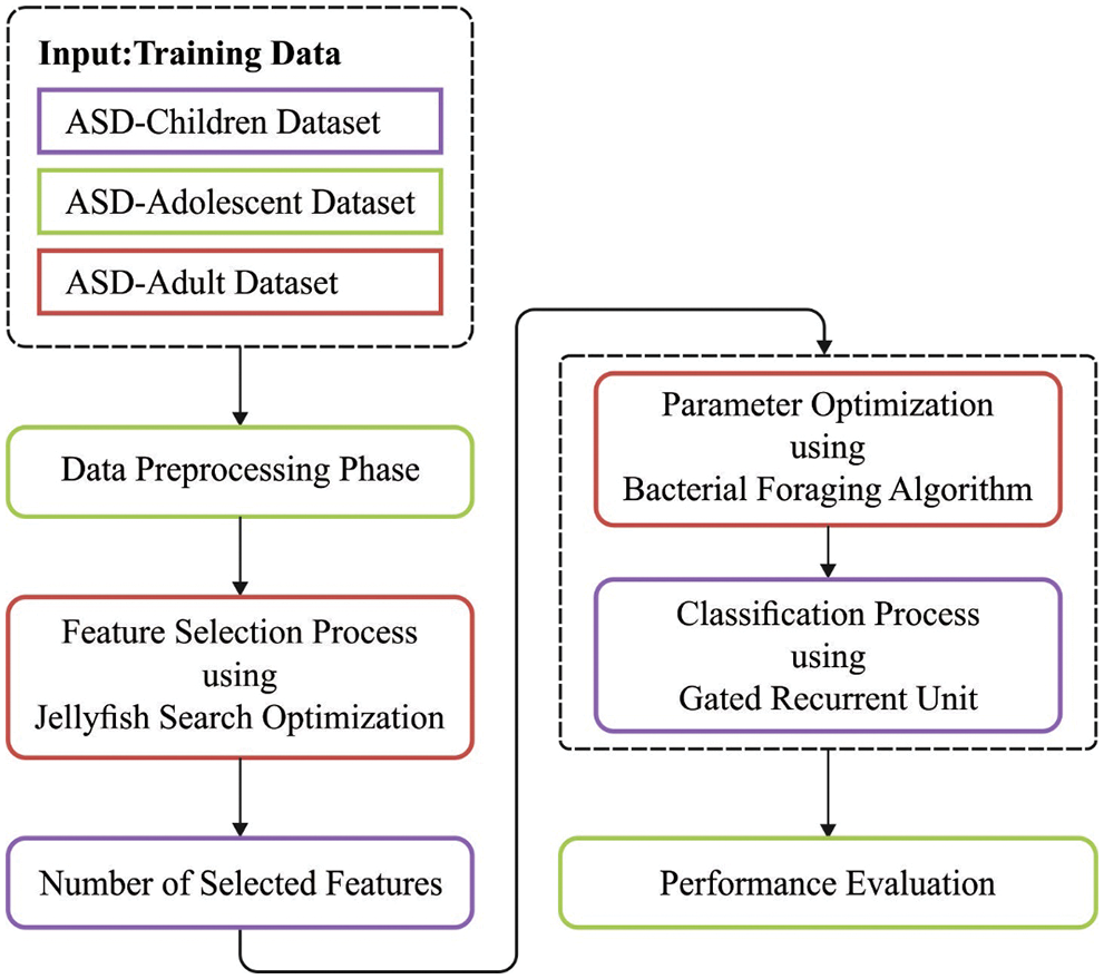
Figure 1: Overall process of JSODL-ASDDC technique
2.1 Process Involved in JSO-FS Technique
In this work, the JSODL-ASDDC model executed JFSO-FS process to choose optimal feature subsets. JSO technique that is a novel Meta-heuristic optimization algorithm that is stimulated by the actions of jellyfish in the ocean [17]. The approach balances the initialized exploration of the searching region and the exploitation to determine the potential region in the searching area (global optimal). A time control mechanism manages the switches among the 2 stages. The control parameter of the procedure is the amount of iterations and population size. The procedure is briefly discussed in the following. Jellyfish move inside the swarm or follows ocean current. In the following, it can be mathematically expressed
From the equation,
Motion of jellyfish in swarm can be categorized as passive (type A) or active (type B). Passive motion in the swarm primarily takes place and it is formulated as follows:
In Eq. (4),
In Eq. (5), f indicates an objective function of position
Therefore,
Here
Time control function switches among motion towards an ocean current, and motion with a jellyfish swarm. It is formulated as follows:
when
Here
2.2 ASD Detection and Classification
Once the features are chosen, the GRU based classification model is utilized for the recognition and classification of ASD. The GRU is a variant of LSTMNN that could resolve the problem of gradient vanishing appeared in the conventional RNN [18]. The GRU method can able to learn long-term dependency dataset of sequential time and automatically determine the optimum time delay. The input of GRU is given as:
In Eq. (9),
The target of GRU is to attain the predictive values of the following time steps without indicating how much time steps must be found. The elementary component of hidden neurons is the GRU memory block. They include resetting gate
In Eq. (12),
2.3 BFO Based Hyperparameter Optimization
In the final stage, the BFO assisted parameter tuning process [19–21] gets executed to improve the efficacy of the GRU model. The standard BFO methodology has two significant facts [22]:
Initiation of solution space: the mapping function
Initiation of Bacterial: the bacteria amount was chosen using S. The position of
Therefore, the fitness value of
From the above formula, the smaller value of function denotes maximal fitness. i indicates the
It has a large number of flipping and swimming activities. In
However, the swimming step length of
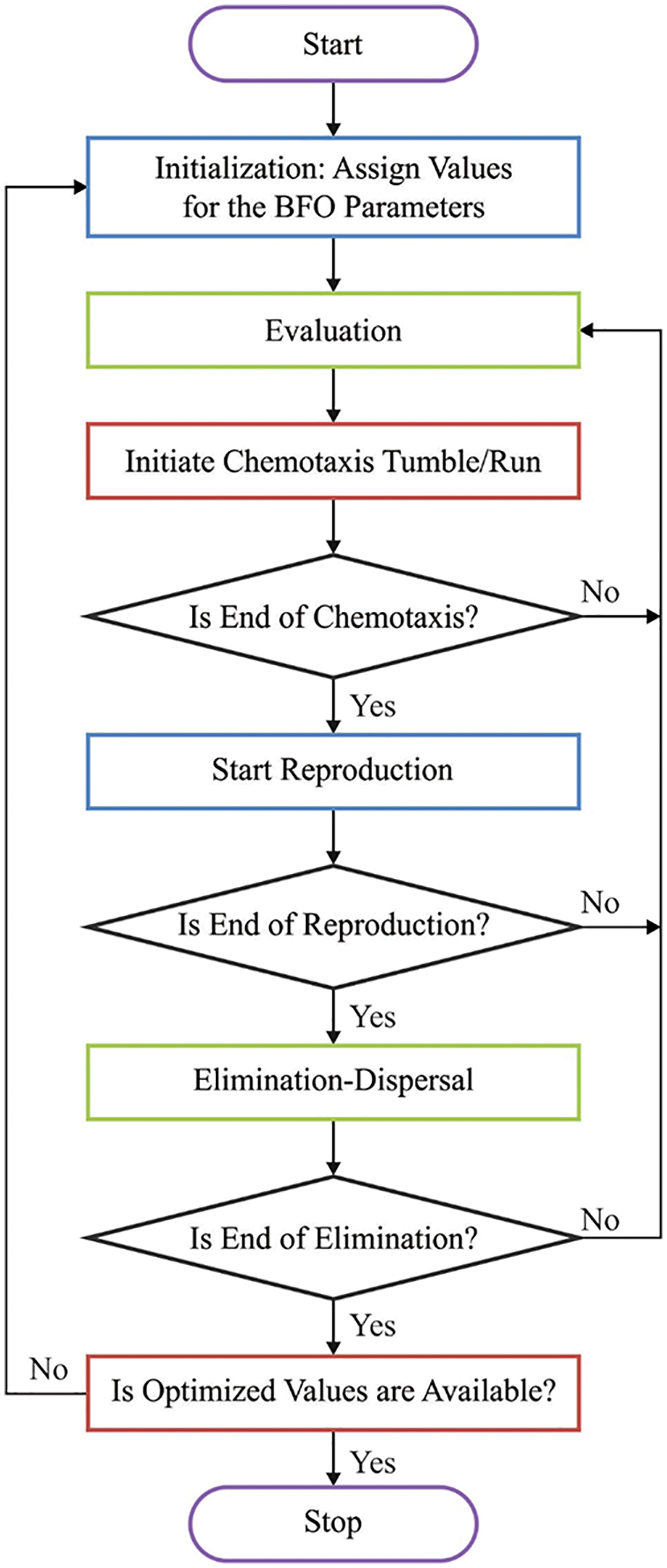
Figure 2: Flowchart of BFO technique
The bacteria are taken into account as attraction and repulsion. The numerical relationship was determined by the following expression:
In Eq. (17),
The bacteria replication as soon as it could accomplish an improved atmosphere; or else, it will pass away. Consequently, with the swarming and chemotaxis methodologies, the fitness of bacteria was fixed and it is calculated. The fitness of
Half of the bacteria are in improved condition
2.3.4 Elimination and Dispersal
Following the reproduction, each bacterium is distributed with likelihood of
As previously mentioned in the above equation, eradication takes place then
The simulation analysis of the JSODL-ASDDC system is tested using three datasets such as ASD-children, ASD-adolescent, and ASD-Adult datasets. Each dataset holds samples under two classes with 21 features.
Fig. 3 illustrates the FS outcome of the JSFO-FS model with other FS models on test data. The results implied the JSFO-FS model has obtained optimal best cost of 0.2937 whereas the QODF-FS, GWO-FS, PSO-FS, GA-FS, and PCA-FS models have portrayed increased best cost of 0.3127, 0.6523, 0.7891, 0.8167, and 0.9208 respectively.
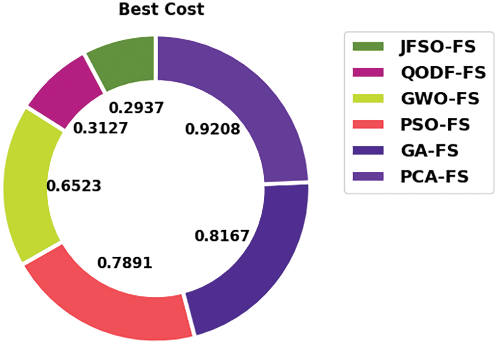
Figure 3: Best cost analysis of JSFO-FS technique
Fig. 4 exemplifies the confusion matrices formed by the JSODL-ASDDC algorithm the test data. With ASD-children dataset, the JSODL-ASDDC model has identified 140 samples in Yes class and 149 samples in No class. In addition, with ASD-adult dataset, the JSODL-ASDDC algorithm has identified 176 samples in Yes class and 513 samples in No class. In line with, with ASD-adolescent dataset, the JSODL-ASDDC technique has identified 61 samples in Yes class and 41 samples in No class.
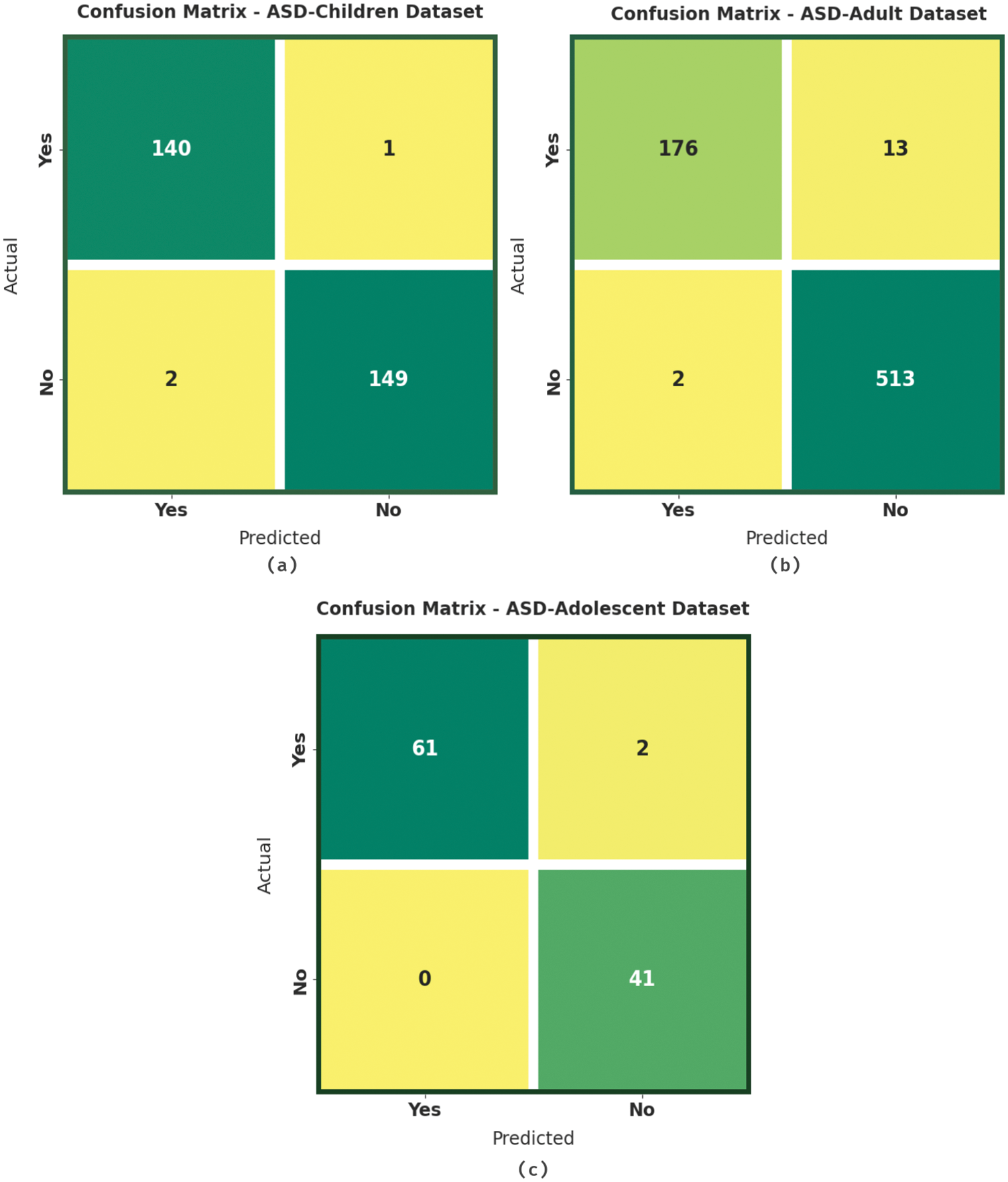
Figure 4: Confusion matrices of JSODL-ASDDC technique (a) ASD-children dataset, (b) ASD-adult dataset, and (c) ASD-adolescent dataset
Tab. 1 offers detailed classification outcomes of the JSODL-ASDDC model with three distinct datasets.
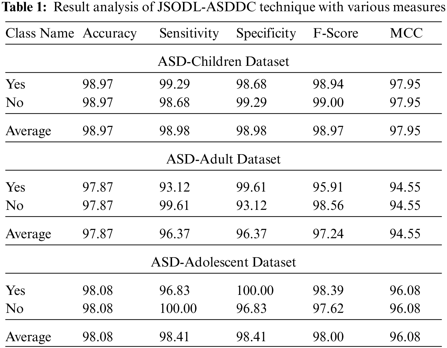
Fig. 5 portrays an overall classifier results of the JSODL-ASDDC model under ASD-children dataset on two class labels. The figure reported that the JSODL-ASDDC model has effectually recognized the samples under two classes. For instance, the JSODL-ASDDC model has identified samples under Yes class with

Figure 5: Result analysis of JSODL-ASDDC technique under ASD-children dataset
Fig. 6 displays the overall classifier outcomes of the JSODL-ASDDC system under ASD-adolescent dataset on two class labels. The figure stated that the JSODL-ASDDC methodology has effectually recognized the samples under two classes. For example, the JSODL-ASDDC method has identified samples under Yes class with
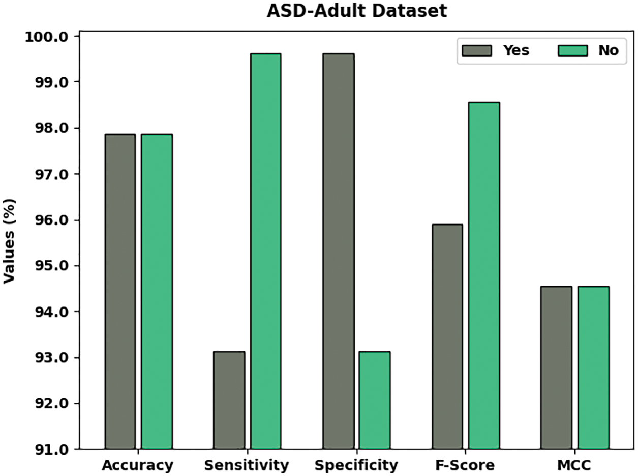
Figure 6: Result analysis of JSODL-ASDDC technique under ASD-adolescent dataset
Fig. 7 represents the overall classifier results of the JSODL-ASDDC system under ASD-adult dataset on two class labels. The figure reported that the JSODL-ASDDC techniques have effectually recognized the samples under two classes. For example, the JSODL-ASDDC model has identified samples under Yes class with

Figure 7: Result analysis of JSODL-ASDDC technique under ASD-adult dataset
Fig. 8 provides a brief comparative study of the JSODL-ASDDC model with other models in terms of
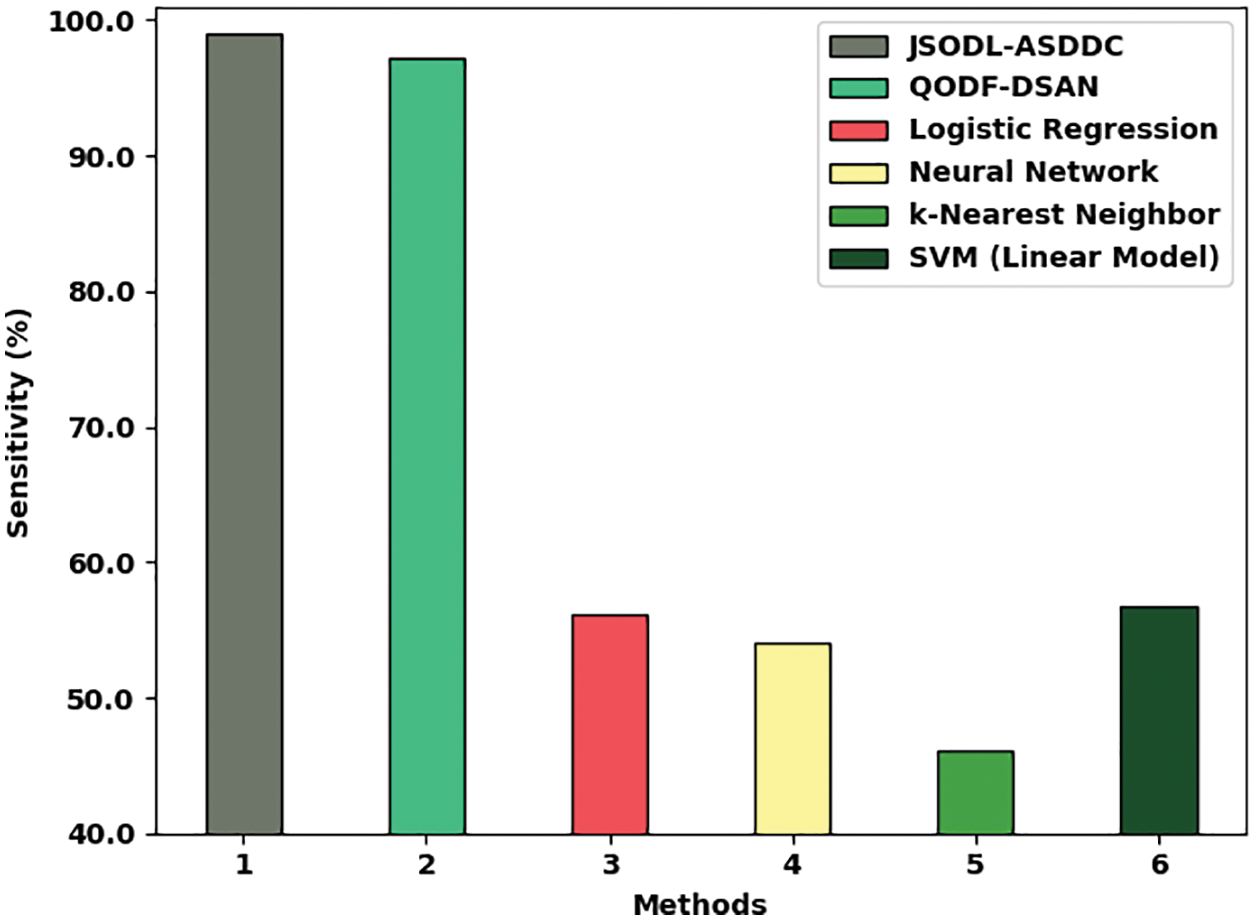
Figure 8:
Fig. 9 offers a brief comparative study of the JSODL-ASDDC algorithm with other models with respect to

Figure 9:
Fig. 10 provides a brief comparison study of the JSODL-ASDDC system with other models in terms of
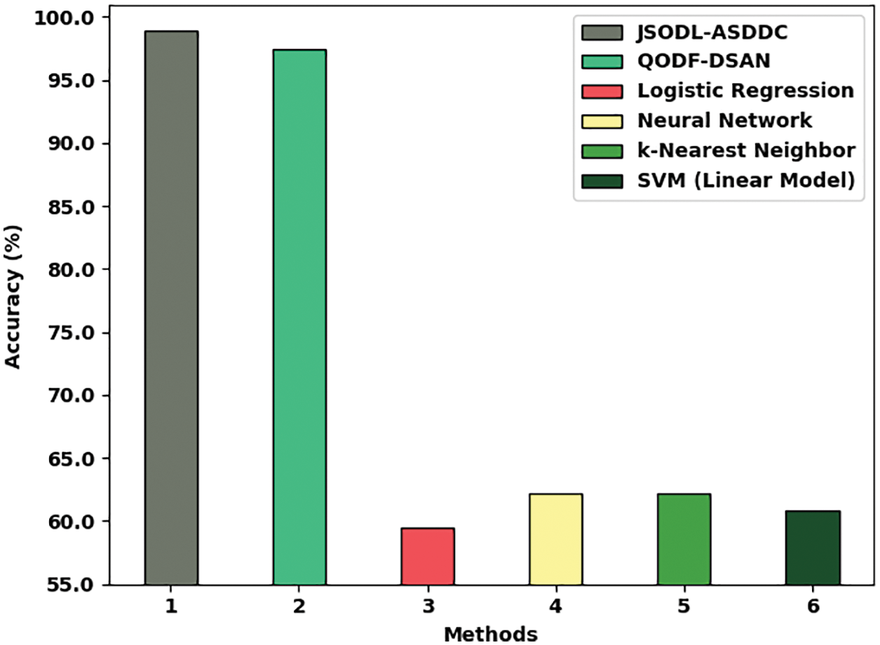
Figure 10:
In this article, a new JSODL-ASDDC algorithm was advanced to identify the different stages of ASD using biomedical data. The proposed JSODL-ASDDC model initially performed min-max data normalization approach to scale the data into uniform range. Followed by, the JSODL-ASDDC model executing JFSO-FS process to choose optimal feature subsets. Then, the BFO-GRU classification model is utilized for the recognition and classification of ASD. Furthermore, the BFO assisted parameter tuning process gets executed to advance the efficacy of the GRU algorithm. The experimental assessment of the JSODL-ASDDC methodology is investigated against distinct datasets. The experimental resultants emphasized the enhanced performance of the JSODL-ASDDC methodology over recent approaches. As a part of future extension, the performance of the JSODL-ASDDC model can be improved by ensemble voting process.
Funding Statement: The authors received no specific funding for this study.
Conflicts of Interest: The authors declare that they have no conflicts of interest to report regarding the present study.
References
1. K. K. Hyde, M. N. Novack, N. LaHaye, C. P. Pelleriti, R. Anden et al., “Applications of supervised machine learning in autism spectrum disorder research: A review,” Review Journal of Autism and Developmental Disorders, vol. 6, no. 2, pp. 128–146, 2019. [Google Scholar]
2. F. Thabtah, “Machine learning in autistic spectrum disorder behavioral research: A review and ways forward,” Informatics for Health and Social Care, vol. 44, no. 3, pp. 278–297, 2019. [Google Scholar]
3. S. Raj and S. Masood, “Analysis and detection of autism spectrum disorder using machine learning techniques,” Procedia Computer Science, vol. 167, pp. 994–1004, 2020. [Google Scholar]
4. J. Bhola, R. Jeet, M. M. M. Jawarneh and S. A. Pattekari, “Machine learning techniques for analysing and identifying autism spectrum disorder,” in Artificial Intelligence for Accurate Analysis and Detection of Autism Spectrum Disorder, IGI Global, Pennsylvania, United States, pp. 69–81, 2021, https://doi.org/10.4018/978-1-7998-7460-7.ch005. [Google Scholar]
5. E. Stevens, D. R. Dixon, M. N. Novack, D. Granpeesheh, T. Smith et al., “Identification and analysis of behavioral phenotypes in autism spectrum disorder via unsupervised machine learning,” International Journal of Medical Informatics, vol. 129, pp. 29–36, 2019. [Google Scholar]
6. M. M. Rahman, O. L. Usman, R. C. Muniyandi, S. Sahran, S. Mohamed et al., “A review of machine learning methods of feature selection and classification for autism spectrum disorder,” Brain Sciences, vol. 10, no. 12, pp. 949, 2020. [Google Scholar]
7. A. M. Pagnozzi, E. Conti, S. Calderoni, J. Fripp and S. E. Rose, “A systematic review of structural MRI biomarkers in autism spectrum disorder: A machine learning perspective,” International Journal of Developmental Neuroscience, vol. 71, no. 1, pp. 68–82, 2018. [Google Scholar]
8. M. D. Hossain, M. A. Kabir, A. Anwar and M. Z. Islam, “Detecting autism spectrum disorder using machine learning techniques: An experimental analysis on toddler, child, adolescent and adult datasets,” Health Information Science and Systems, vol. 9, no. 1, pp. 17, 2021. [Google Scholar]
9. T. Akter, M. S. Satu, M. I. Khan, M. H. Ali, S. Uddin et al., “Machine learning-based models for early stage detection of autism spectrum disorders,” IEEE Access, vol. 7, pp. 166509–166527, 2019. [Google Scholar]
10. N. Chaitra, P. A. Vijaya and G. Deshpande, “Diagnostic prediction of autism spectrum disorder using complex network measures in a machine learning framework,” Biomedical Signal Processing and Control, vol. 62, pp. 102099, 2020. [Google Scholar]
11. K. S. Omar, P. Mondal, N. S. Khan, M. R. K. Rizvi and M. N. Islam, “A machine learning approach to predict autism spectrum disorder,” in 2019 Int. Conf. on Electrical, Computer and Communication Engineering (ECCE), Cox’sBazar, Bangladesh, pp. 1–6, 2019. [Google Scholar]
12. H. S. Nogay and H. Adeli, “Machine learning (ML) for the diagnosis of autism spectrum disorder (ASD) using brain imaging,” Reviews in the Neurosciences, vol. 31, no. 8, pp. 825–841, 2020. [Google Scholar]
13. M. Liao, H. Duan and G. Wang, “Application of machine learning techniques to detect the children with autism spectrum disorder,” Journal of Healthcare Engineering, vol. 2022, pp. 1–10, 2022. [Google Scholar]
14. X. Yang, N. Zhang and P. Schrader, “A study of brain networks for autism spectrum disorder classification using resting-state functional connectivity,” Machine Learning with Applications, vol. 8, pp. 100290, 2022. [Google Scholar]
15. M. R. Alteneiji, L. Mohammed and M. Usman, “Autism spectrum disorder diagnosis using optimal machine learning methods,” International Journal of Advanced Computer Science and Applications, vol. 11, no. 9, pp. 252–260, 2020. [Google Scholar]
16. K. D. C. Garside, Z. Kong, S. W. White, L. Antezana, S. Kim et al., “Detecting and classifying self-injurious behavior in autism spectrum disorder using machine learning techniques,” Journal of Autism and Developmental Disorders, vol. 50, no. 11, pp. 4039–4052, 2020. [Google Scholar]
17. E. A. Gouda, M. F. Kotb and A. A. E. Fergany, “Jellyfish search algorithm for extracting unknown parameters of PEM fuel cell models: Steady-state performance and analysis,” Energy, vol. 221, pp. 119836, 2021. [Google Scholar]
18. R. Fu, Z. Zhang and L. Li, “Using LSTM and GRU neural network methods for traffic flow prediction,” in 2016 31st Youth Academic Annual Conf. of Chinese Association of Automation (YAC), Wuhan, China, pp. 324–328, 2016. [Google Scholar]
19. K. Shankar, E. Perumal, M. Elhoseny, F. Taher, B. B. Gupta et al., “Synergic deep learning for smart health diagnosis of COVID-19 for connected living and smart cities,” ACM Transactions on Internet Technology, vol. 22, no. 3, pp. 16:1–14, 2022. [Google Scholar]
20. M. Y. Sikkandar, B. A. Alrasheadi, N. B. Prakash, G. R. Hemalakshmi, A. Mohanarathinam et al., “Deep learning based an automated skin lesion segmentation and intelligent classification model,” Journal of Ambient Intelligence and Humanized Computing, vol. 12, no. 3, pp. 3245–3255, 2021. [Google Scholar]
21. K. Shankar, A. R. W. Sait, D. Gupta, S. K. Lakshmanaprabu, A. Khanna et al., “Automated detection and classification of fundus diabetic retinopathy images using synergic deep learning model,” Pattern Recognition Letters, vol. 133, pp. 210–216, 2020. [Google Scholar]
22. Y. P. Chen, Y. Li, G. Wang, Y. F. Zheng, Q. Xu et al., “A novel bacterial foraging optimization algorithm for feature selection,” Expert Systems with Applications, vol. 83, pp. 1–17, 2017. [Google Scholar]
23. M. N. Parikh, H. Li and L. He, “Enhancing diagnosis of autism with optimized machine learning models and personal characteristic data,” Frontiers in Computational Neuroscience, vol. 13, pp. 9, 2019. [Google Scholar]
24. G. D. Varshini and R. Chinnaiyan, “Optimized machine learning classification approaches for prediction of autism spectrum disorder,” Annals of Autism & Developmental Disorders, vol. 1, no. 1, pp. 1001, 2020. [Google Scholar]
Cite This Article
 Copyright © 2023 The Author(s). Published by Tech Science Press.
This work is licensed under a Creative Commons Attribution 4.0 International License , which permits unrestricted use, distribution, and reproduction in any medium, provided the original work is properly cited.
 Downloads
 Citation Tools