Estimating Construction Material Indices with ARIMA and Optimized NARNETs

1  Introduction

Construction Industry operates relying on different economic indicators ranging from construction material prices to sales volumes and prices. Nearly all economic indicators have temporal (time-dependent) nature. The stakeholders in the industry either employers/investors or contractors/suppliers keep close eye on economic indicators to decide whether to start a new project, to complete a project in a planned or longer time period or abandon a project completely (to prevent bankruptcy). As the construction industry related economic indicators change over time, forecasts regarding these indicators are made using different econometric models, and mostly with time series analysis. For instance, indicators such as cost indices, price indices and sales volumes can be estimated using time series analysis [1–4]. Construction cost is a key concern in construction management. It is crucial for construction companies to know about the future variation of construction prices. In conditions with low certainty, reliable cost forecasts become an important source of information for decision making. Material cost is one of the key components of the overall cost of construction. Increasing the accuracy of material price prediction can improve the accuracy of cost estimates, as around ¼ of the total cost of construction projects is the material cost [5]. Estimation of material cost is known to be a difficult task due to the material price fluctuations during the construction period [6]. Thus, in order to carry out a successful cost management strategy it becomes important to find reliable methods for the estimation of construction material prices. In addition, cost overrun is a common problem in the construction industry, where 9/10 of construction projects face cost overrun [7,8]. Cost overrun causes numerous issues in the construction projects’ performance. Cost overrun occurs either due to a change in material/workforce prices or by a change order. Building materials have a huge impact on the costs of construction projects. The literature states that the major cause of cost overrun is the price increase of construction materials [9]. To prevent cost overruns in the projects, the estimation of material prices is of critical importance.

To increase the foreseeability of the costs of construction materials, this study focuses on estimation of construction material indices. Time series analysis has been chosen as the estimation approach as the indicators of the indices have a time-dependent nature. Two different types of analysis are implemented for estimation of the future values of the indicators of material indices. The first approach was Box-Jenkins (ARIMA) method which is known to be successful in estimation of time series having a linear nature. The second method implemented was Non-Linear Autoregressive Neural Network (NARNET) which is known to be successful in modeling and estimation of series with non-linear components along with a linear nature. In addition, in this study, we have developed a grid search algorithm (for identifying best hyperparameters for the network) and an accompanying software tool to explore an optimal NARNET architecture for realizing most accurate estimation with NARNETs. Following the background section on the use of time series analysis techniques in construction industry, an exploratory analysis of the data is provided. This is followed by an elaboration on the details of ARIMA and NARNET based estimation procedures. In the final sections the results of the analysis are presented and discussed.

2  Background

According to the literature, ARIMA models were used in many fields for different purposes including economics, to model and predict the exchange rates [10,11], to model and predict stock market movements [12–14], for forecasting in the crypto money market [15,16], in agriculture for predicting production and consumption [17–19] and in the health sector to model expenditures and to predict the spread of pandemic diseases [20,21]. ARIMA based (linear) and ANN based (non-linear) methods have also been implemented and tested for different purposes in construction industry. For instance, [22] used the Box-Jenkins model technique to model and predict three different variables of the construction industry in Singapore, namely tender price, construction demand, and industry-level productivity. The first model deals with public industrial building tender prices, the second model deals with residential construction demand, and the third model deals with construction efficiency at the industry level. Each of these case studies served a different purpose to meet the specific needs of the Singapore construction industry. For the first case, a total of 49 quarterly data from 1980-Q1 and 1992-Q1 were used. The first 47 quarters formed the modeling dataset, while the remaining 2 quarters were used to test the model’s accuracy for out-of-sample predictions. The second case study consisted of a total of 77 observations from the first quarter of 1975 to the first quarter of 1994. The first 72 quartiles were used to generate the modeling dataset and the remaining 5 quartiles were used for out-of-sample estimates. The third case study consisted of a total of 22 observations from 1975 to 1996. The first 20 periods were used for modeling and the last two periods were used for testing. Two accuracy measures were adopted, root mean-square-error (RMSE) and mean absolute percentage error (MAPE). The results show that the predictive RMSE of all three models is consistently smaller than the model’s standard error, indicating that the models have good predictive performance. Among these models, the lowest MAPE value belongs to the demand model, followed by the price model and the efficiency model.Reference [23] used quarterly time series statistics for the period 1983Q1–2002Q4 to analyze and forecast five key indicators in the Hong Kong construction labor market. The variables used in the models were employment level, productivity, unemployment rate, underemployment rate and real wage. The data used in the analysis were collected by the HKSAR Government’s Department of Census and Statistics (C&SD). The first 80 quarters created the modeling dataset to build the forecast model, while the remaining five quarters were used to evaluate the model for out-of-sample forecasts. According to the results, MAPE and Theil U statistics showed good predictive performance in majority of models, except for the construction employment situation. Among the five models, the most accurate was the construction real wage model. Finally, multivariate structural forecasting analysis should be adopted to obtain accurate estimates of construction employment in Hong Kong.Reference [24] focused on estimating the quarterly total gross value of residential, commercial, industrial, and total construction output using ARIMA models with quarterly data from 1983Q1 to 2008Q1. According to the results, Box-Jenkins models reliably predicted medium-term aggregate construction demand and housing demand covering increases and decreases in construction demand. The purpose of [25] was to compare the accuracy of Autoregressive Integrated Moving Average (ARIMA) and Autoregressive Neural Network (ARNET) models. Four quarterly time series datasets from C&SD between 1983Q1 and 2014Q4 were used to predict fluctuations in the construction industry. The results show that the ARNET model is a reliable estimation method for aggregate, private and other construction outputs in the medium term. It is found out the ARNET outperforms the ARIMA model in terms of accuracy.Reference [26] aimed to improve the Construction Cost Index (CCI) estimation performance by addressing the long memory concept. For this purpose, the presence of long memory in CCI was investigated by performing a rescaled interval analysis on data from 1990-January and 2016-August. Then, the Autoregressive Fractional Integrated Moving Average (ARFIMA) model, which reflects the characteristics of long memory, was fit to the data. According to the results, ARFIMA’s forecast performance outperformed ARIMA by an average of 9.5%. The ARFIMA model has achieved higher CCI prediction performance with the features of long memory.Reference [27] used Artificial Neural Networks (ANN), Linear Regression and Autoregressive Time Series (ARIMA) methods to estimate CCI. These three models were used to predict the CCI until 2025. With the MAPE value of 3.5, ARIMA was found as the most accurate method.Reference [28] aimed to estimate the number of people injured in occupational accidents in the construction industry in Poland between 2007 and 2019. A mathematical model was created in the nonlinear regression class. The model provided a high-accuracy estimation of the number of people injured in the construction industry in certain years and months. The prediction errors obtained from models such as ARIMA, Seasonal ARIMA (SARIMA), linear and polynomial models, and the errors obtained from the developed model were compared. The mean estimation error for the developed model was found as 8.9%, and this demonstrated that the developed model reflects the randomness phenomenon in the construction industry well and is performing better than linear and polynomial regression, ARIMA, SARIMA models.Reference [29,30] proposed an ARIMA-ANN model to estimate construction costs and investigated whether this model can have higher accuracy than the solo ARIMA or solo ANN model. Construction cost indices were estimated for short, medium and long-term forecast periods using ARIMA, ANN and ARIMA-ANN models. According to the results, it was determined that the ARIMA-ANN model performs better than other models for long-term forecasting periods.Reference [31] aimed to help managers find and analyze the factors affecting the construction cost estimation to make good decisions. The research was focused on analyzing construction costs from the point of adopting multivariate cost prediction models in predicting construction cost index (CCI) and other independent variables from September 2021 to December 2022. Independent variables include Building Permits (BP), Consumer Price Index (PPI), Unemployment Rate (UNEMP), Employment Rate (EMP), Crude Oil Prices (BOIL), Money Supply (MS), Producer Price Index (PPI), Gross Domestic Products (GDP) and Import Price Index (IPI). SPSS and R applications were used for analysis of the data. According to the results of this research, the ARIMA model was the best predictive model with the highest model-fit correlation. The literature indicates that different linear and non-linear models can be used to represent the relationships of time dependent variables/indicators that are used in the construction industry. The choice of models ranges from ARIMA, SARIMA, ARFIMA to ANN, ARNET and hybrid ARIMA-ANN models. Some studies reported that ANN and ARNET models perform better than ARIMA, but others reported better accuracies with ARIMA models, and a few studies implemented hybrid ARIMA-ANN models and found them more accurate when compared with the others. It can be concluded that in modeling time dependent indicators of the construction industry there is no one-size-fits-all solution or model, and different modeling techniques have to be employed and tested for series of different nature. The following section first provides an exploratory analysis of the data used in this study, and later elaborates on the analysis/modeling techniques implemented.

3  Methodology

3.1 The Dataset

The Association of Turkish Construction Material Producers (IMSAD) was founded in 1984 acts as an organization that represents Construction Materials Industry both in Turkey and internationally. IMSAD has 85 industrial (company) and 52 industry association members. The association follows developments in the domestic market closely, and also keeps close track of foreign markets for increasing the continuity of success in material exports. IMSAD is well known with its Construction Material Industry Indices which are published on a monthly basis. The main index is known as the Compound Index and is composed of 3 main index groups, Activity Index Group, Expectation Index Group, and Trust Index Group. The Activity Index Group is composed of 6 indictors (A1.Domestic Sales, A2.Production, A3.Exports, A4.Endorsement, A5.Collection Rate, A6.International Sales Price) the Expectation Index Group is composed of 7 indicators focusing on expectations regarding next 3 months (E1.Expection from Economy in General, E2.Expectation from Construction Material Industry, E3.Expectation of Domestic Orders, E4.Expectation of Export Orders, E5.Expectation of Production, E6.Expectation of New Production Capacity Investments, E7.Expectation for Employment) and Trust Index Group is composed of 5 indicators (T1.General Course of Economy, T2.General Course of Construction Industry, T4.General Trend in Domestic Markets, T3.General Trend in Construction Materials Industry, T5.General Trend in Export Markets. The value of each indicator is determined on a monthly basis, based on responses to indicator questions (which are sent to members of the association periodically each month). The values of the indicators for a specific month have been calculated by taking 100 as the reference (base) value which refers to the indicator value of August 2013 (base year/month).

In this study, we collected monthly data that cover the period from 2013:8 to 2021:3 regarding all indicators A (1–6), E(1–7) and T(1–5). Fig. 1 provides time series plots of 18 indicators grouped by index groups Activity (A), Expectation (E) and Trust (T).

Figure 1: Time series plots of indicators

Following the examination of the time series plots, in order to identify the stationarity of the time series at level (i.e., diff = 0), Autocorrelation Plots of all indicators were generated and examined. The autocorrelation plots indicated that all series show signs of non-stationarity at Level as the values do not tend to degrade to zero quickly (e.g., in 3–4 lags) in all of the graphics (Fig. 2).

Figure 2: Autocorrelation plots of indicators at level (diff = 0)

In the following phases of the research the applicability of Box-Jenkins (ARIMA) method and Optimized NARNETs in making future predictions of the indicators are tested. The tests started with a proof-of-concept exercise to demonstrate the applicability of Box-Jenkins Method for a selected (solo) indicator. Later a toolbox is developed and tested to facilitate future predictions of all indicators by exploring, finding, and utilizing Optimized NARNETs.

In the start of the modeling process, to efficiently validate the results, the data is divided into training and testing sets. The training set covered the period between 08.2013–06.2019 (71 obs.) and the test set covered the period between 07.2019–03.2021 (21.obs). The Root Mean Square Error (RMSE) and Mean Absolute Error (MAE) are used as the performance metrics of the models in all training and validation stages.

3.2 Estimation with Box-Jenkins (ARIMA) Method

Following the exploratory analysis of the data we employed the Box-Jenkins methodology for forecasting the values of a selected (solo) indicator. The indicator to be estimated is determined as E1, as a result of examination of Autocorrelation Function (ACF) (Fig. 2) and Partial Autocorrelation Function (PACF) plots of all variables. In this examination, the E1 indicator was showing the strong signs of fitting to an ARIMA (Auto-regressive Integrated Moving Average) model equation. As illustrated in Fig. 3, ACF and PACF plots of the series, the series E1 is not stationary at level (I ≠ 0) and both ACF and PACF plots of first difference of the E1 series tend to degrade into the confidence interval quickly i.e., at 1–2 lags. Following the examination of ACF and PACF plots of E1 series, a range of ARIMA (p, d, q) models (p: 0 to 3, d: 1 to 2, q: 0 to 3) have been fit through a grid search with (p × d × q: 4 × 2 × 4) 32 runs of the ARIMA model fit in EViews 10 using the training dataset (71 obs.). Depending on the Akaike information criterion (AIC), the best ARIMA model representing the E1 training set was found as ARIMA (2, 1, 1).

Figure 3: ACF and PACF plots of E1 at level (diff = 0) and first difference (diff = 1)

3.3 Estimation with Optimized NARNETs

ARIMA models are used to model linear relationships in data. In fact, most time series are characterized by high variations and rapid transient periods, thus a nonlinear approach should be used to model these type of time series. As indicated in [32–34] it was demonstrated that a time series can also be modeled and represented by a nonlinear autoregressive (NAR: Nonlinear Auto-Regressive) model. As explained in [33] the classical Recurrent Neural Network (RNN) encounters some difficulties when faced with problems with long period dependence which is the case for time series. These difficulties originate in the gradient descent problem, and this is the case for all recurrent networks other than Non-Linear Autoregressive Neural Network (NARNET). This makes NARNET very suitable for use in modeling and predicting time series with non-linear components. A Nonlinear Auto-Regressive Neural Network, NARNET, is a RNN which forms a discrete, nonlinear, autoregressive system with endogenous inputs. The equation for the network can be written as [33] (Eq. (1)).

y(t)=h(y(t−1),y(t−2),…,y(t−p))+ε(t)(1)

The equation explains how a NARNET can be utilized to predict the value of series y at time t, y(t), using the (p) past values of the series. The function h(.) is unknown in advance, and the training of the NARNET aims to approximate the function by means of the optimization of the weights and biases. The error term ε(t) stands for the error of the approximation of the series y at time t. NARNET is a multilayer, recurrent, dynamic network, with feedback connections. In a NARNET the terms y(t − 1), y(t − 2), . . . , y(t − p), are known as feedback delays (Fig. 4).

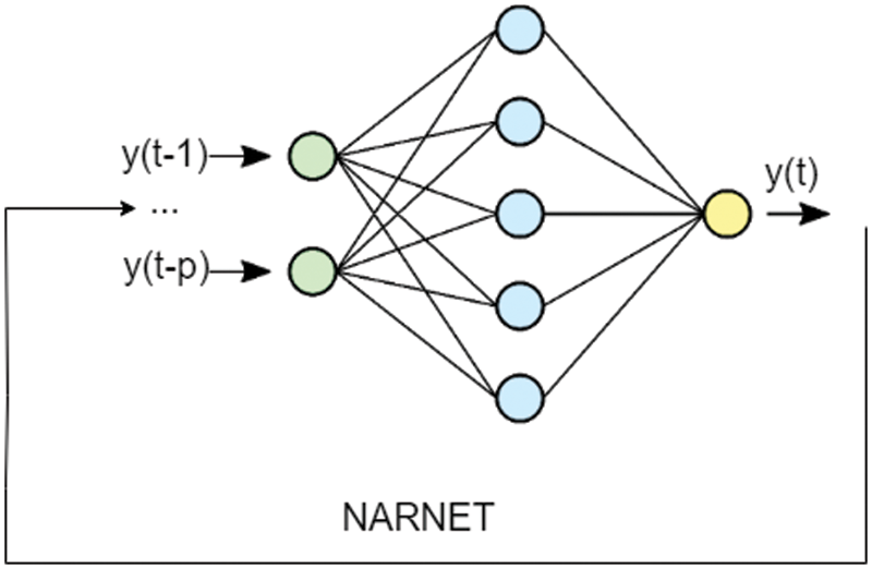
Figure 4: NARNET architecture

The most commonly used learning rule for the NAR Network (NARNET) is the Levenberg-Marquardt backpropagation procedure (LMBP) [32]. The Levenberg-Marquardt algorithm combines two numerical minimization algorithms: the gradient descent method and the Gauss-Newton method. In the gradient descent method, the sum of the squared errors is reduced by updating the parameters in the steepest-descent direction. In the Gauss-Newton method, the sum of the squared errors is reduced by assuming the least squares function is locally quadratic in the parameters and finding the minimum of this quadratic. The Levenberg-Marquardt method acts more like a gradient-descent method when the parameters are far from their optimal value and acts more like the Gauss-Newton method when the parameters are close to their optimal value [35]. As explained in [36] the Levenberg-Marquardt algorithm was designed to approach second-order training speed without having to compute the Hessian matrix. This algorithm appears to be the fastest method for training moderate-sized feedforward neural networks (up to several hundred weights). The procedure has an efficient implementation in MATLAB software, as the solution of the matrix equation is a built-in function, so its attributes become even more pronounced in a MATLAB environment. The original description of the Levenberg-Marquardt algorithm is given in [37]. The application of Levenberg-Marquardt to neural network training is described in [38].

In this study we propose and implement a grid search algorithm to find the most accurate NARNET (NARNET with minimum errors) through optimizing its hyperparameters. The training function used to train the network was chosen as LMBP as it the most commonly used function in the training of NARNETs. The hyperparameters used as the input of our objective function were i.) the size of hidden layer and ii.) the number of feedback delays. The training can be repeated N times to achieve better accuracies, and the number of epochs in each training are adjusted/determined automatically by the LMBP based training of NARNET in MATLAB. The accuracy of the model in our algorithm is calculated on the basis of test set. The pseudocode of the grid search algorithm is given in Listing 1.

Listing 1. Grid-search algorithm

function findBestNARNET (trainset, testtest hiddenlayer_size_items, feedbackdelay_no, training_repeat)

best_rmse ← high_positive_value

best_mae ← high_positive_value

bestnet, best_record, best_rsqr

       for i ← 1 to feedbackdelay_no

              for j ← 1 to hiddenlayer_size_item

                  for k ← 1 to training_repeat

                        [training_record, trained_net] = train_network (trainset)

                        predictions = trainednet.predict (testset)

                        [rmse, mea, rsqr] = calculate_metrics (testset, predictions)

                        if best_rmse > rmse & best_mae > mae

                         bestnet ← trained_net

                         best_record ← training_record

                         best_rmse ← rmse

                         best_mea ← mae

                         best_rsqr ← rsqr

                        end if

                  end

              end

       end

return bestnet, best_record, best_rmse, best_mea

end function

The grid search algorithm has been implemented in MATLAB and embedded in a tool developed by the authors. The tool developed is a MATLAB App and provides a Graphical User Interface (GUI) which can be used in data preparation, entry of hyperparameter options, training, and visualization of the results. The tool consists of 3 parts. The first set of parameters (Prepare Data Tab) focuses on data preparation for optimal network search. The data can be loaded in form of an Excel or CSV file by using the “Load Data” command from the toolbar menu. Once loaded, the unprocessed/raw data is visualized in a Data Table at the lower part of the window. The column in focus (i.e., the series in focus when there are multiple series) can be determined as data column using this interface, and once determined the data column is illustrated with blue color. A cut-point row can be determined also here. The cut point row, once determined, indicates where to separate the data into train and test sets. The last row of the training set to be prepared is colored in red, while the first row of the test set to be prepared is colored in yellow. Graph View switch is used to provide a time series plot of the data. Once this switch is On, any click on the data column would provide a time series plot of the data as an image. Differencing (Δ) can be applied to the data if the data has trend or seasonality to remove these effects. The data preparation interface allows the user to apply first (Δ1) or second (Δ2) order differencing to the dataset. (Fig. 5) Once all data preparation parameters have been determined and input into the system the toolbar command “Prepare Data” is used to generate the training and test sets. These sets are stored as arrays in the MATLAB environment, and are visualized, and can be controlled using the user interface.

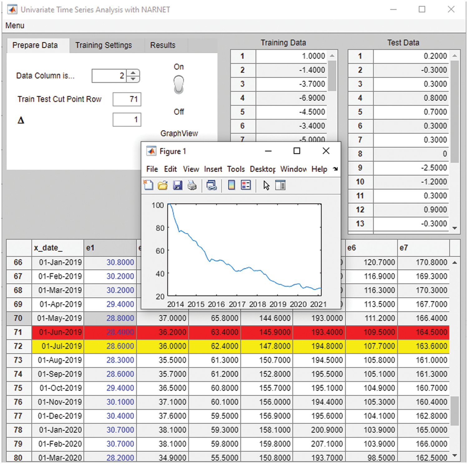
Figure 5: Data preparation and first set of input parameters

The second set of parameters is for inputting the hyperparameter boundaries that would be used in the grid search to find the optimal NARNET, in parallel with the algorithm provided in Listing 1. In Listing 1, two hyperparameters form the search space (number of feedback delays and hidden layer size), and each configuration of combination of these two hyperparameters can be run N times. The user can input Feedback Delays parameter as an integer value (f), which indicates that the grid search will be conducted between 1 and (f) feedback delays for all different hidden layer sizes. Secondly the user can provide an array of “Hidden Layer Sizes”, which indicates that the grid search will consider each hidden layer size provided in this array, for instance if this array is [5 10 15], this indicates that the grid search will take single layer NARNETs with 5, 10, and 15 neurons into account (for each feedback delay) during the search for the optimal model. A training configuration (a single combination of a feedback delay and hidden layer size e.g., [1, 5] or [5, 10]) can be run N times in order to repeat the LMBP based training process of the NARNET N times. Each of these runs would result in similar networks in terms of architecture (number of neurons, feedback delays) but with different weights and biases determined in each run, and thus having different accuracies (RMSE, MAE scores). Running a training configuration multiple times increases the chance of finding the optimal (most accurate) NARNET for each configuration. Thus, this step contributes to the grid search not as an hyperparameter, but by deeply searching the best weight-bias combination for each hyperparameter configuration. The user can input number of times the training configuration will be run, i.e., run of each config, among the second set of parameters (Fig. 6). The training is run by selecting the “Train” command on the toolbar menu. Once the training is complete a figure showing the optimal network architecture is displayed if the “View Best Network” switch is On.

Figure 6: Second set of input parameters

The third set of parameters provides the accuracy metrics calculated for the optimal NARNET. These parameters are RMSE/MAE (and R2, the supplementary measure). These are calculated for each iteration using the test set during the optimal model search (see Listing 1). Once the training is complete, and the optimal (most accurate) model is determined, its accuracy metrics are displayed in the third parameter set (Results Tab). At the completion of the training, the training record is logged by MATLAB and the optimal network is saved, both as MATLAB environment variables. The optimal network saved can later be used for further validation studies with different training and test sets to further assess its performance (Fig. 7).

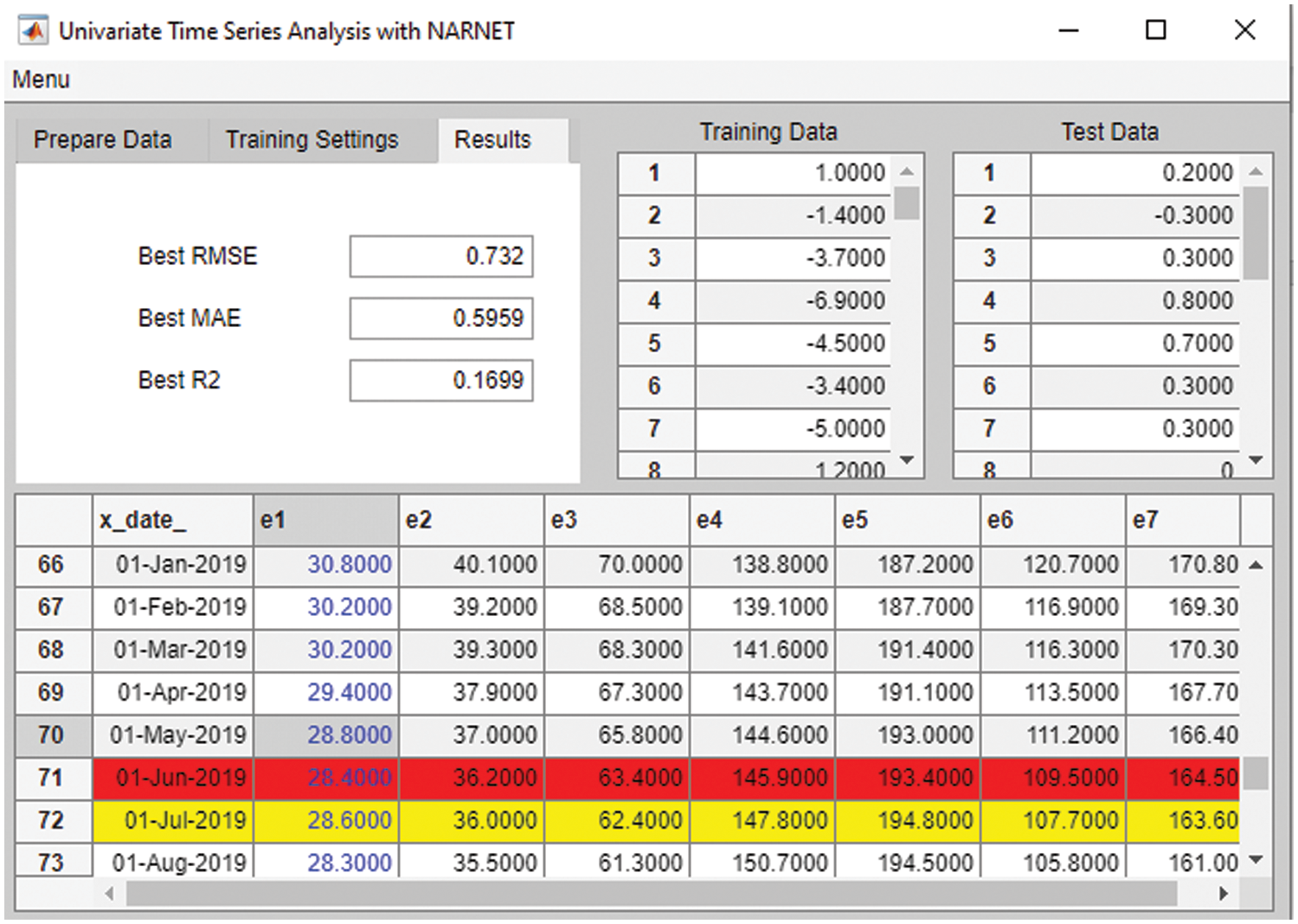
Figure 7: Accuracy metrics

Once all the training and tests are complete, we evaluated the results achieved through Box-Jenkins (ARIMA) and Optimal NARNET search methods, the next section of the paper elaborates on the numerical results and provides a discussion on applicability of these techniques for estimation of Construction Material Indices.

4  Results and Discussion

4.1 Box Jenkins (ARIMA) Model Outputs

As a result of 32 rounds of analysis with EViews 10 explained previously, the estimated coefficients of the best fit ARIMA model is shown in Tab. 1, and the equation of the ARIMA Model is provided in Eq. (2).

wt=1.2434wt−1−0.3480wt−2+εt+0.9999εt−1−0.5923wt=Δ1y=yt−yt−1(2)

Following this, we estimated the i.) Training Set through Static (in-of-sample) and Dynamic (out-of-sample) estimation methods, and ii.) Test Set through Static (in-of-sample) and Dynamic (out-of-sample) estimation methods. The accuracy metrics for all these estimations are provided in Tab. 2, and Fig. 8 provides a time series plot showing the original and estimated series.

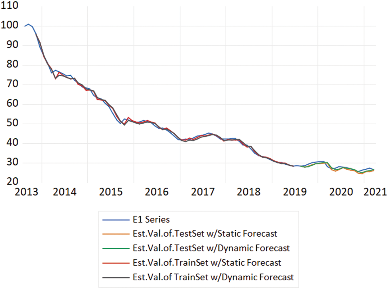
Figure 8: Time series plot of original and estimated series

4.2 The Outputs of Optimal NARNET Models

Following the Box-Jenkins (ARIMA) modeling process of E1, all indicators have been modeled and estimated with the optimal NARNETs (discovered by the MATLAB App developed during this study). As the Autocorrelation Plots of Indicators at Level (Fig. 2) illustrates, all indicator variables were not stationary at level, thus first difference of all variables is used in generation of training and test sets for estimation. The training set covered the 09.2013–06.2019 period (70 obs.), while the test sets covered the period between 07.2019–03.2021 (21 obs.). In-of-sample (static) estimation method is used in the estimation process. In terms of range of hyperparameters, feedback delays evaluated by the networks were [1, 2, 3, 4], hidden layer sizes evaluated were [15, 20, 25] and each training configuration has been run 5 times. Tab. 3 provides the summary of the estimation results with hyperparameters of optimal NARNETs.

In order to compare the performance of ARIMA and NARNET models, the estimation accuracies for E1 were checked. For the test set of E1, the static forecast of the ARIMA model results in RMSE:1.0157, and MAE: 0.8917, while the static forecast of the NARNET model results in RMSE:0.710 and MAE:0.585. The NARNET model has significantly lower error rates when compared with ARIMA model, RMSE: 0.881 σ vs. RMSE 1.26 σ, and MAE:0.726 σ vs. MAE:1.106 σ.

When all estimations with NARNET models complete, it is observed that the model accuracies in terms of RMSE range between 0.552 σ–1.145 σ, and in terms of MAE, they range between 0.444 σ–0.880 σ. The results indicate that when optimal network delays were found more than one (i.e., 1:2 or 1:3) the series tend to have a relatively high variance (e.g., A1, A4, E2, E3), but not all series with high variance (e.g., E5, A2) have been modelled optimally with networks having delays more than one. Thus, it is not possible to argue that a correlation in optimal models exists between series variance and number of network delays input into the system. The majority of the number of neurons in the hidden layer of optimal networks were 15 (lowest alternative evaluated). This might be related to the size of training sets (70 obs.), where low complexity in networks provide better estimation results of small datasets (following the law of parsimony). The results also demonstrated that regardless of the nature and complexity of the time series data, NARNETs are able to model the time-dependent relationship in data with success, which would not be the case for solo use of linear models such as ARIMA.

5  Conclusion

Cost is a key concern in the operations of the construction industry, material costs has a huge impact on the overall cost of construction. In order to foresee the trends of the cost of construction materials, this study concentrated on estimation of construction material indices. The literature indicates that in modeling time dependent indicators of the construction industry there is no one-size-fits-all solution or model, and different modeling techniques have to be employed and tested for series of different nature. In our study, the estimation of construction material indices is accomplished through ARIMA and Non-Linear Autoregressive Neural Network (NARNET) methods. The estimation with Box-Jenkins (ARIMA) Methodology has been done for the E1 indicator, where an ARMA model is fitted to the first difference of the E1 series. The static (in of sample) estimation of the test set of E1 resulted with RMSE 1.26 σ and MAE:1.106 σ, which can be considered as a good accuracy. Following this, optimal NARNET architectures for all indicators have been identified through a grid search algorithm (developed for identifying best hyperparameters for the network) and utilizing an accompanying software tool. The optimal NARNET models provided better accuracies, for instance, the static (in of sample) estimation of the test set of E1 resulted with RMSE: 0.881 σ and MAE:0.726 σ. The algorithm and accompanying MATLAB App developed demonstrated that grid search can be efficiently used in finding the NARNETs with optimal hyperparameters. The study results have demonstrated that depending on the nature of the series, both methods can successfully and accurately estimate the future values. The proposed approach presents a new direction and method in estimation of construction material price indicators. The developed tool can be used by construction industry professionals and cost managers to efficiently estimate trends related to material prices which would lead to take more effective estimation of material prices and this in turn would enhance the foreseeability of the material costs in the construction industry.

Funding Statement: This research was supported by the Energy Cloud R&D Program through the National Research Foundation of Korea (NRF) funded by the Ministry of Science, ICT (2019M3F2A1073164) and MSGSU BAP (2021-25).

Conflicts of Interest: The authors declare that they have no conflicts of interest to report regarding the present study.

References

1. C. Tunçay, “Türkiye’de konut sektöründeki ortalama karlılığın konut yatırımlarına ve konut fiyatlarına etkisi,” Politik Ekonomik Kuram., vol. 4, no. 2, pp. 242–254, 2020. [Google Scholar]
2. S. Gözübüyük and A. Koy, “Türkiye’de konut üretiminin belirleyicileri: Ekonomik büyüme ve konut faiz oranı,” Bankacılık ve Sermaye Piyasası Araştırmaları Dergisi, vol. 4, no. 9, pp. 1–10, 2020. [Google Scholar]
3. G. A. Karaağaç and S. Altınırmak, “Türkiye konut fiyat endeksi ve düzey bazli konut fiyat endeksleri ile seçili değişkenler arasindaki nedensellik ilişkisi,” Karadeniz Uluslararası Bilimsel Dergi, vol. 39, no. 39, pp. 222–240, 2018. [Google Scholar]
4. H. Karadaş and E. Salihoglu, “Seçili makroekonomik değişkenlerin konut fiyatlarına etkisi:Türkiye örneği,” Ekonomik ve Sosyal Araştırmalar Dergisi, vol. 16, no. 1, pp. 63–80, 2020. [Google Scholar]
5. S. Hwang, M. Park, H. S. Lee and H. Kim, “Automated time-series cost forecasting system for construction materials,” Journal of Construction Engineering and Management, vol. 138, no. 11, pp. 1259–1269, 2012. [Google Scholar]
6. M. Mir, H. M. Dipu Kabir, F. Nasirzadeh and A. Khosravi, “Neural network-based interval forecasting of construction material prices,” Journal of Building Engineering, vol. 39, pp. 1–13, 2021. [Google Scholar]
7. B. Flyvbjerg, N. Bruzelius and W. Rothengatter, Megaprojects and Risk: An Anatomy of Ambition, Cambridge, United Kingdom, Cambridge University Press, 2003. [Google Scholar]
8. A. Aljohani, D. Ahiaga-Dagbui and D. Moore, “Construction projects cost overrun: What does the literature tell us?” International Journal of Innovation, Management and Technology, vol. 8, no. 2, pp. 137–143, 2017. [Google Scholar]
9. M. A. Musarat, W. S. Alaloul, M. S. Liew, A. Maqsoom and A. H. Qureshi, “Investigating the impact of inflation on building materials prices in construction industry,” Journal of Building Engineering, vol. 32, pp. 1–14, 2020. [Google Scholar]
10. A. S. Babu and S. K. Reddy, “Exchange rate forecasting using ARIMA neural network and fuzzy neuron,” Journal of Stock & Forex Trading, vol. 4, no. 3, pp. 1–5, 2015. [Google Scholar]
11. P. Escudero, W. Alcocer and J. Paredes, “Recurrent neural networks and ARIMA models for Euro/Dollar exchange rate forecasting,” Applied Sciences, vol. 11, no. 12, pp. 1–12, 2021. [Google Scholar]
12. Y. Wang and Y. Guo, “Forecasting method of stock market volatility in time series data based on mixed model of ARIMA and XGBoost,” China Communications, vol. 17, no. 3, pp. 205–221, 2020. [Google Scholar]
13. Y. Musa and S. Joshua, “Analysis of ARIMA-artificial neural network hybrid model in forecasting of stock market return,” Asian Journal of Probability and Statistics, vol. 6, no. 2, pp. 42–53, 2020. [Google Scholar]
14. H. Öcal, S. İmre and A. A. Kamil, “The sell in may effect: An empirical analysis from Turkey, Indonesia, France and Germany,” Hong Kong Journal of Social Sciences, vol. 58, pp. 239–251, 2021. [Google Scholar]
15. M. Khedmati, F. Seifi and M. J. Azizi, “Time series forecasting of bitcoin price based on autoregressive integrated moving average and machine learning approaches,” International Journal of Engineering, vol. 33, no. 7, pp. 1293–1303, 2020. [Google Scholar]
16. Z. H. Munim, M. H. Shakil and I. Alon, “Next-day bitcoin price forecast,” Journal of Risk and Financial Management, vol. 12, no. 2, pp. 1–15, 2019. [Google Scholar]
17. G. M. Tinungki, “The election of the best autoregressive integrated moving average model to forecasting rice production in Indonesia,” Advances and Applications in Statistics, vol. 52, no. 4, pp. 251–265, 2018. [Google Scholar]
18. M. Ray, V. Ramasubramanian, A. Kumar and A. Rai, “Application of time series intervention modelling for modelling and forecasting cotton yield,” Statistics and Applications, vol. 12, no. 1, pp. 61–70, 2014. [Google Scholar]
19. J. F. Mgaya, “Application of ARIMA models in forecasting livestock products consumption in Tanzania,” Cogent Food & Agriculture, vol. 5, no. 1, pp. 1–29, 2019. [Google Scholar]
20. S. I. Alzahrani, I. A. Aljamaan and E. A. Al-Fakih, “Forecasting the spread of the COVID-19 pandemic in Saudi Arabia using ARIMA prediction model under current public health interventions,” Journal of Infection and Public Health, vol. 13, no. 7, pp. 914–919, 2020. [Google Scholar]
21. M. Ramezanian, A. A. Haghdoost, M. H. Mehrolhassani, M. Abolhallaje, R. Dehnavieh et al., “Forecasting health expenditures in Iran using the ARIMA model (2016–2020),” Medical Journal of the Islamic Republic of Iran, vol. 33, pp. 1–4, 2019. [Google Scholar]
22. G. B. Hua and T. H. Pin, “Forecasting construction industry demand, price and productivity in Singapore: The Box–Jenkins approach,” Construction Management and Economics, vol. 18, no. 5, pp. 607–618, 2000. [Google Scholar]
23. J. M. Wong, A. P. Chan and Y. H. Chiang, “Time series forecasts of the construction labour market in Hong Kong: The Box-Jenkins approach,” Construction Management and Economics, vol. 23, no. 9, pp. 979–991, 2005. [Google Scholar]
24. R. Y. Fan, S. N. Thomas and J. M. Wong, “Reliability of the Box–Jenkins model for forecasting construction demand covering times of economic austerity,” Construction Management and Economics, vol. 28, no. 3, pp. 241–254, 2010. [Google Scholar]
25. K. C. Lam and O. S. Oshodi, “Forecasting construction output: A comparison of artificial neural network and Box-Jenkıns model,” Engineering Construction and Architectural Management, vol. 23, no. 3, pp. 302–322, 2016. [Google Scholar]
26. S. Moon, S. Chi and D. Y. Kim, “Predicting construction cost index using the autoregressive fractionally integrated moving average model,” Journal of Management in Engineering, vol. 34, no. 2, pp. 1–12, 2017. [Google Scholar]
27. Y. Elfahham, “Estimation and prediction of construction cost index using neural networks, time series, and regression,” Alexandria Engineering Journal, vol. 58, no. 2, pp. 499–506, 2019. [Google Scholar]
28. B. Hoła, M. Topolski, I. Szer, J. Szer and E. Borowa-Blazik, “Prediction model of seasonality in the construction industry based on the accidentality phenomenon,” Archives of Civil and Mechanical Engineering, vol. 22, pp. 1–13, 2022. [Google Scholar]
29. C. Y. Choi, K. R. Ryu and M. Shahandashti, “Predicting city-level construction cost index using linear forecasting models,” Journal of Construction Engineering and Management, vol. 147, no. 2, pp. 1–12, 2021. [Google Scholar]
30. S. Kim, C. Y. Choi, M. Shahandashti and K. R. Ryu, “Improving accuracy in predicting city-level construction cost indices by combining linear ARIMA and nonlinear ANNs,” Journal of Management in Engineering, vol. 38, no. 2, pp. 1–14, 2022. [Google Scholar]
31. F. Jiang, J. Awaitey and H. Xie, “Analysis of construction cost and investment planning using time series analysis,” Sustainability, vol. 14, no. 3, pp. 1–16, 2022. [Google Scholar]
32. L. G. B. Ruiz, M. P. Cuéllar, M. D. Calvo-Flores and M. D. C. P. Jiménez, “An application of non-linear autoregressive neural networks to predict energy consumption in public buildings,” Energies, vol. 9, no. 9, pp. 1–16, 2016. [Google Scholar]
33. M. Ibrahim, S. Jemei, G. Wimmer and D. Hissel, “Nonlinear autoregressive neural network in an energy management strategy for battery/ultra-capacitor hybrid electrical vehicles,” Electric Power Systems Research, vol. 136, pp. 262–269, 2016. [Google Scholar]
34. O. Allaf and S. A. Kader, “Nonlinear autoregressive neural network model for estimation soil temperature: A comparison of different optimization neural network algorithms,” in IEEE Int. Conf. on Industrial Technology, Auburn, USA, pp. 43–51, 2011. [Google Scholar]
35. H. P. Gavin, “The Levenberg-Marquardt algorithm for nonlinear least squares curve-fitting problems,” 2020. [Online]. Available: https://people.duke.edu/~hpgavin/ce281/lm.pdf (accessed on 25 Apr. 2022). [Google Scholar]
36. MATLAB, “MATLAB implementation of the Levenberg-Marquardt algorithm,” 2022. [Online]. Available: https://www.mathworks.com/help/deeplearning/ref/trainlm.html. [Google Scholar]
37. D. Marquardt, “An algorithm for least-qquares estimation of nonlinear parameters,” Journal of the Society for Industrial and Applied Mathematics, vol. 11, no. 2, pp. 431–441, 1963. [Google Scholar]
38. M. T. Hagan and M. Menhaj, “Training feed-forward networks with the Marquardt algorithm,” IEEE Transactions on Neural Networks, vol. 5, no. 6, pp. 989–993, 1994. [Google Scholar]
Cite This Article
Copyright © 2023 The Author(s). Published by Tech Science Press.
This work is licensed under a Creative Commons Attribution 4.0 International License , which permits unrestricted use, distribution, and reproduction in any medium, provided the original work is properly cited.
Downloads
Citation Tools