Impact of Portable Executable Header Features on Malware Detection Accuracy

1  Introduction

Many implementations have incorporated the Portable Executable (PE) header features to search for malware inside such files. It was proved by more than one implementation that some or many of those features can be employed to differentiate between benign and malicious files. Each work implements a strategy in studying and extracting the features that may affect the accuracy in detecting the malware. In previous implementations there were some observations that needed to be studied and proved like the number of features used, combinations of the feature set and the specific features used may also affect the accuracy level. This work will study those observations.

This work assumed that the selected features that will be used have the required positive impact on accuracy, this was assumed according to previous observation. Selecting the features was not just a matter of collecting a random feature set. It was also assumed that the number of features can be reduced and accuracy can be improved, also the combination of features and incorporating particular features could affect the accuracy positively, again this was not a random assumption it was based on some previous indications that needed to be proved.

Causing harm intentionally through changing, adding, or removing code from software to destroy its intended function is considered as malware. Significant limitations can be found in malware detection technology, despite numerous conducted studies [1].

A variety of techniques has been implemented by modern malware detectors [2]. The file type is determined first by the detector, then finding items that are embedded in the file and/or extracting its content to parse the file. So, a variety of formats needs to be parsed by the anti-virus scanner, this will lead to complex antivirus software. In certain cases, even sophisticated anti-virus software cannot capture a simple malware.

Machine learning utilizes the behavioral and structural features of both benign and malware files in the malware classification model building process. This model will identify the samples as being good or infected [3]. Different Portable Executable header features were incorporated to discriminate infected from good files, observations of [3] showed that larger differences to infected and benign files were for values of NumberOfSymbol, SizeOfInitialized Data and NumberOfSections.

Originally, Win32 native executable format is a Portable Executable (PE). PE specifications were derived from the UNIX Common Object File Format (COFF) the necessary information is encapsulated inside the data format structure that represents the PE. That information is used for the MS-Windows operating system loader, so that the management of the executable code can be carried out [4]. Unfortunately, Portable Executable (PE) format were not designed to be a code modification resistant; because of that the malware injection process is easy. The infection will happen when a code that is malicious is injected into a portable executable. By infecting the PE file, many threats like ransomware, Trojans and worms will start working. Once the PE files are infected the malware can run without giving any indications to the user.

According to [5], various cyber-attacks are threatening computer networks, system admins of those networks utilize Intrusion Detection tools, Deep-Packe Inspection (DPI) and Encryption to guard against such threats. Today machine learning can also be used to further improve security.

Many previous implementations discussed the differences between a traditional method of detecting malware using Signature-based techniques and a machine-learning-based technique; it is mentioned in [6] and [7] that the static technique of signature-based block already recognized malware, unfortunately, this will be difficult regarding fresh malware. Several Anti-malware programs use a second technique which is a dynamic technique based on using virtual environments to run the executable on, this technique has a major drawbacks mainly high resource consumption and a lengthy scanning duration.

A third technique utilized today that incorporates machine learning, is the heuristic technique, which has proven its success in many fields [6,7]. A comparison in [8] and [9] has been made between signature-based and machine-learning techniques, concluding that machine-learning technique can deduce benign and malicious samples and use the appropriate parameters for the detection model. The work of [8] mentioned that malware detection is no longer passive due to introducing machine learning. It is stated in [10] that a major problem with signature-based methods used nowadays is that it is ineffective to face the zero-day attack and every minute lost in waiting for updating the anti-virus software or signature files, is another time that their computers are vulnerable to damage. Also, obfuscation can be used to bypass the examination operation of a virus scan in a signature-based malware detection [11].

The Authors of [12] implemented a hybrid technique which incorporated signature and machine learning techniques to protect Internet of Things (IoT) systems against attacks coming from home Wi-Fi devices. The system could stop five big attack types classified as top ten vulnerabilities in 2018.

According to [11], the software can be protected using the executable packer tool, this tool originally can be used to protect important information against reverse engineering. Unfortunately, packing has become a tool for obfuscation, using encryption or compression techniques, the malware shape can be changed so that detection mechanisms such as heuristic analysis will be confused. Statically, 80% of malware was packed not only to confuse the signature-based malware detectors, but also to propagate the compact form malware.

On the other hand, a hiding information system is presented by [13], this system will hide the data file inside image page of a .exe file (execution file). This system solved the problems of detecting the .exe file as a virus and that the .exe file is still working, since hiding data inside the .exe file may change the functionality of the executable file itself.

According to [2], a standardization for the PE file format was established by the MS-Windows operating system for dynamically linked libraries (DLL), object files and executable files. The work [2] suggested an accurate and real-time framework for PE-Miner. The framework can extract distinguished features automatically from PE to inspect malware. Results obtained after completing a single pass were more than 99% detection rate with less than 0.5% false alarm rate, but time cost was about one hour to scan the whole content of the PE file.

In [4], twenty-nine PE file header features were collected, the work employed AI to study these features as means of finding malware and evaluate their effect on accuracy. Two different classification algorithms were used in that study.

According to previous observations which showed that features of the PE header file when incorporated in detecting malware can either have a positive or negative effect on the malware detection accuracy; this work studied the different circumstances that could affect the accuracy, like the number of features, the collection of the features used, if there are some particular features which have more impact on accuracy than others and if it is possible to reach the optimized set of features which always can be used to discriminate between benign and malware files. This required a strategy in selecting the features in each run. Subgrouping the features according to previous observations and putting a criterion that defined the high accuracy, good accuracy and low accuracy, were the main factors that affect the process of reaching the aims of this work.

The reminder of this paper will include the following: Section 2 introduces the related work. Section 3 presents why targeting portable executable in this work. Section 4 will explain the utilized algorithms. Section 5 will present work criteria. Section 6 illustrates work methodology presenting the subgrouping method. Section 7 will discuss results with charts. Section 8 will present a discussion that includes work observation and a comparison to previous work and finally, conclusions will be presented in Section 9.

2  Related Work

Many implementations aimed at avoiding hazards due to the misuse of PE files, using different aspects to detect malware.

The Authors of [9] incorporated several machine learning models k-Nearest Neighbors (kNN), Support-Vector Machine (SVM) and Random Forest; an accuracy of 95.59% was achieved. The obtained accuracy was due to using only nine features, the utilized values were with a significant difference between benign and malware-infected files. It is stated that the proposed model’s speed is high which leads to faster training for the model.

The Authors of [14] proposed a smaller set of attributes to discover malware. In that way, researchers replaced the method of identifying malware with thousands of attributes using a single model. As they believe, that utilizing smaller attribute sets, will lead to reduced processing overload, this will be accomplished by reducing the number of files required to extract thousands of attributes. Using the VirusTotal tool and by keeping their model up to date, the model produced a 97% accuracy.

An approach to differentiate malware and benign .exe files was introduced in [2], the approach was by looking at the properties of the MS-Windows PE header and extracting the features used to differentiate between the two by using the structural information of MS-Windows related to these files. Three steps to accomplish that were used: (1) from two websites a large dataset was collected regarding legitimate and malware .exe files, (2) comparing benign and malware files was made after extracting the features of each header file and (3) after extracting icons from the PE file the most prevalent of these were found.

The important role of features in a PE file is presented in [15], the work argued the detection of packed executables using those features. Packing will change the portable executable; it will produce a file that will be difficult to investigate either being benign or malicious. So, the study took packed executables only, extracted them, then analyzed its features to reach the best set of features which will conclude whether a binary file is packed or not.

To detect malware J. Bai et al. [1] suggested the feature information mining, this work incorporated slightly less than 200 features, those features were extracted from portable executable files and then trained using a classification algorithm, a 99.1% accuracy with 97.6% of new malware detection was obtained.

The Authors of [16] considered the effect of employing numerous obfuscation techniques which led to the evasion of malware detection. The work claimed that traditional approaches to detecting malware like signature scanning became ineffective. Researchers illustrated that the obfuscation affected the PE file and some anomalies have been introduced. The work studied the importance of static heuristic features and used fuzzy classification algorithms, so that an attempt to detect malware and packed file can be made.

Emphasizing on obtaining accurate decisions for malware classification and intrusion attacks through selecting and extracting features were done by [17]. The work was conducted using machine learning and designing systems that can understand, prevent and detect malicious connections. Combining features that can use packet history for correlation.

The Authors of [3] involved machine learning in files classification to be malware or benign, with low computational overhead and high accuracy. A combination of executable header fields, raw and derived values were created from merging integrated feature sets. Various machine learning algorithms were employed to classify malware, for example KNN, Logistic Regression, Decision Tree, Random Forest, Naïve Bayes and Linear Discriminator Analysis. An accuracy of 98.4% was obtained using ten-fold cross-validation using the proposed integrated features. Using the top 15 features only 97%–98% accuracy was obtained on raw and integrated features respectively.

Raff et al. [18] used the minimal amount of domain knowledge to be able to extract portion of the PE header. This was the suggestion in applying the neural networks to help detecting malware and learning features.

Deep learning together with Artificial Immune System (AIS) were used in [19] to classify a file to be benign or malware aiming to employ a high rate of accuracy. This work was implemented in two stages, first, the extraction of PE headers and establishing a feature set. Then building generation of malware detectors is done in the second stage using AIS. The accuracy rate detection of unknown virus was improved. As a result, 99.4% detection rate was achieved.

Maleki et al. [20], applied a forward selection method after feature extracting to detect malware. After that file classification is done to conclude either benign or malware, using different classification methods. The Decision Tree (DT) classifier achieved the highest results with an accuracy of 98.26%.

The Authors of [4] employed Neural Networks and Decision Tree after testing some clustering and classification algorithms, 29 features were collected from previous implementations. The study added a feature at a time and recorded accuracy after each addition of that feature. Results obtained were as follow: using Neural network with test_size of 0.3 and random_state of 10, a feature set of 21 features and another set of 28 features both produced an accuracy of 0.9781; for Neural Network with test_size of 0.15 and random_state of 3, a feature set of 23 features produced an accuracy of 0.9796. For the Decision Tree with test_size of 0.3 and random_state of 10, a feature set of 25 features produced 0.9845 accuracy. As for the Decision Tree with test_size of 0.15 and random_state of 3, a feature set of 19 features produced 0.9874 accuracy.

The Authors of [21] proposed a malware detection and classification based on n-grams attribute similarity, also the researchers used C4.5 Decision Tree, Bayesian Networks, Support Vector Machine and Naïve Bayes in addition to the proposed system. Deep Q-learning Network (DQN) was used in [8], by analyzing features using neural networks, then the action space and the corresponding Q-Value are extracted, based on that and by using Q-Learning a decision strategy action is selected, hence detection of malware is complete. The authors of [22] suggested the use of resource-friendly and advanced analysis for malware forensics procedure. The procedure incorporates the static analysis principles which can be used to detect the purpose of an executable exactly. The proposed method attained a higher accuracy in exploring the format of portable executable.

The Authors of [23] used different methods of fuzzy hashing to detect similarities in a file by examining specific hashes. Adding to that, this work examined a combination technique that can be used to enhance rates of detection in the hashing method. The hashing methods used in this work were Ssdeep, PeHash and Imphash, also the study focused on the section and file hashing and techniques that calculates the similarity of a portable executable file. Results showed that improved detection rates were obtained by using evidence combination techniques.

The Authors of [24] implemented the Portable Executable File Analysis Framework (PEFAF) technique. While Static analysis was used by [25] which was used to extract the set of integrated features, this set was created through combining some raw features taken from three headers of PE files and derived features set. The learning process of [25] used seven supervised algorithms to implement the malware classification. Metrics used were accuracy, F-measure and precision. Results showed that integrated feature set has a better performance than the raw feature set on all used metrics. Accuracies between 91% and 99% were produced by integrated feature set, while accuracies between 71% and 97% were produced using raw dataset. The split ratio was 70/30. 99.23% was obtained using Random Forest.

Reference [26] used six Tree-Based ensemble machine learning systems. Voting Ensemble Classifier (VEC), Extra Trees Classifier (ETC), Bagging Decision Tree Classifier (BDT), Ada-Boost Classifier (ABC), Gradient Boosting Classifier (GBC) and Random Forest Classifier (RFC). The metadata extracted from the portable executable file was raw and calculated features (54 features), the achieved accuracy was above 95% in all tested classifiers.

A histogram of instruction opcodes was used in [27] to help in metamorphic virus family variants classification. Support Vector Machine (SVM) has been used in [10] as a classification algorithm, the classifier training process is done simultaneously with feature selection, this will reduce attributes number and got a cost-effective classifier performance.

The Authors of [28] stated that packing will alter several portable executable file properties. So, the work proposed a method to improve detection techniques.

A packing detection framework (PDF) is presented by [11] which mentioned that extraction of valued attributes is done and then used to train a two-class SVM (Support Vector Machines) learning classifier to recognize if the executable is packed.

KDD’99 data-set was used in [5] as benchmark in the literature of intrusion detection. Various techniques that incorporated machine-learning techniques were applied to this dataset, to build anomaly-based intrusion detection system.

The work of [29] suggested the use of a hybrid machine learning algorithm, by combining two or more different individual algorithms. A voting classifier, Logistic Regression, LightGBM and XGBoost has been employed. The work used the recall as a performance metric which attained 99.5%. The authors of [30] implemented a static analysis to PE files, then an auto-encoder has been used to detect malware codes. The work had extracted 549 features; those features include information regarding the DLL/API. The work stated that this method is an effective one.

Long Short Term Memory (LSTM) has been used by [31], the LSTM was paired with LightGBM in the classification of malware using PE. A training process was carried out and then tested using the Sophos-ReversingLabs 20 Million Dataset (SoReL-20M). The results obtained were 91.73%. LSTM was also incorporated for Ransomware detection by [32] based on PE file headers, the work stated that important information can be found inside the PE header, especially about the structure of the program. i.e., the changes that can occur to the sequence of bytes constituting the header’s information can change the program structure. The work implemented a method of separating the samples with ransomware and the sequence of bytes forming the header was processed using the LSTM network. The method obtained 93.25% accuracy.

Taking both the attacker’s point of view and the defender’s point of view was carried out by [33], in which IM-AGE_RESOURCE attack which is an adversarial attack method and a malware detection model were proposed. The proposed model employed machine learning and dimension reduction techniques. Evaluation of the model was done by using the surface information of PE from the 2018 FFRI dataset.

Detecting malicious code using deep learning models was done by [34], the work proposed the generative pre-trained transformer based (GPT-2) and stacked bidirectional long short-term memory (Stacked BiLSTM). The .text sections for the benign and malicious PE files contains assembly instructions. Those instructions were extracted and treated as sentence for each instruction, while each .text section was treated as document. Each sentence and document was labeled as either malicious or benign this was done according to the source of the file. Three datasets were created, documents, composed the first one and fed into Document Level Analysis Model (DLAM) based on BiLSTM which is stacked. While the sentences were composing the second dataset and Sentence Level Analysis Models (SLAMs) were using it, this was based on DistilBERT and Stacked BiLSTM, General Language Model GPT-2 (GLM-GPT2) and Domain Specific Language Model GPT-2 (DSLM-GPT2). Finally, and without any labels, all assembly instructions were combined to produce the third dataset. After that a pre-trained custom model was fed with it. Then, a comparison to malware detection performance was done. F1_score metric was used to test the performance.

An investigation to classification accuracy of malware was done by [35]. The process is done using custom log loss function and Based on LightGBM. The learning process is controlled using the LightGBM through installing the α coefficient to the false negative side loss function and β to the false positive loss function. A lopsided classifier was created through installing the α and β coefficients. Two malware datasets were used, a public and a non-public. Dataset features were obtained from PE-header and the analysis of PE-file surface. Those extracted features were customized a function of binary log loss so that an improvement to the performance metrics of the classification process can be done to certain extent. Results obtained were AUC = 0.979 when α = 430 and β = 339.

3  Portable Executable Features

Portable Executable defines both the layout section and executable form. All .dll, .exe and .sys files incorporate portable executable which is in MS-Windows system looks like a data structure with binary form. Portable Executables include the file description’s information that is used by the MS-Windows loader. Adding to that the program code is hosted by the portable executable [36].

Portable Executable (PE) has three different headers the DOS Header, the File header and the optional header, each header includes a set of structures. According to previous implementations, some of these structures are considered to have an impact on accuracy, those structures are used as features. This work collected previously employed structures and used them to carry out the experiments of the work.

Some or many portable executable header features (structures) can be a source of threat to the operating system if they are used to host malware.

According to this fact several works were presented in the field of studying those portable executable header features, different methods were utilized to extract the most sensitive and effective features. Each work suggested a set of features to study, some of the features were common between more than one study such as the DllCharacteristics.

The Authors of [37] utilized eight features, for example, MajorImageVersion, AddressOfEntryPoint and MajorLinkerVersion. According to [36], in 2012 a paper was written by Yibin Liao which incorporated PE-Header-Parser so that parts of the portable executable header can be analyzed, the work found that if checksum, DLLCharacteristics and MajorImageVersion equals to zero, then with 90% accuracy the executable is malware. Also, the software can be malicious if SizeOfInitializedData equal to zero.

The Authors of [19] listed about 25 features, those features can be utilized to obtain better accuracy in malware detection. A combination of raw and binary features was incorporated in [3], an example of raw features used are SizeOfHeaders and SizeOfUninitializedData.

Liao [2] suggested five features as the features which includes the significant differences between benign and malware executables. Those features are UnknownSectionName, DLLCharacteristics, SizeOfInitializedData, Checksum and MajorImageVersion.

This work employed a wide range of features. Majority of the features used by previous implementations except six features, one of them does not apply to the current work, four of them did not appear in the control dataset [38] and the last one has no effect on accuracy after tests were made in this work and previous work [4].

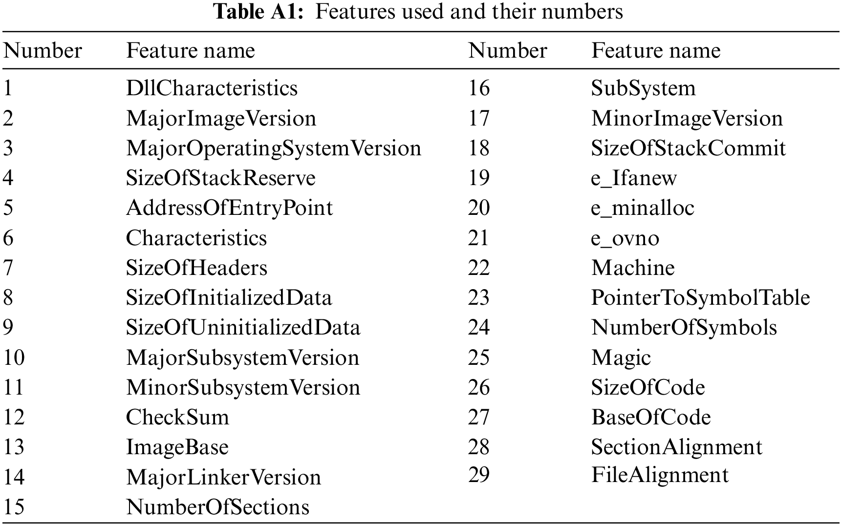
Appendix A include Tab. A1 in which the used features in this work are listed. In this work Feature number in Tab. A1 will replace the feature name.

4  Algorithms Used

Deciding algorithms used in this work was concluded after many tests on different algorithms, some of the tested algorithms were clustering algorithms others were classification algorithms. From the clustering algorithms used in these tests was the K-Means Clustering and from the classification algorithms used were Random Forest, Naïve Bayes and Support Vector Machine (SVM). It is stated in [37] that malware can be better dealt with using a classification approach, hence, two classification algorithms were selected which are Neural Network Multi-Layer Perceptron Classifier (NN_MLPC) and Decision Tree (DT).

Besides the enhanced results obtained from using those two approaches, there are other reasons led to selecting them. Neural Network can handle a human like intelligence, it has the ability to simulate the human brain [39]. Hence, it is possible to build a classifier using a Neural Network algorithm which may achieve better performance in detecting malware in the portable executable file.

With the Decision Tree (DT) predictions are built by considering representing the values in a categorical and numerical forms [37]. Two major reasons behind selecting the Decision Tree, first DT produced the highest results among all the other algorithms tested; Second, many implementations used DT and this gave this technique popularity characteristic.

The performance accuracy metrics formula used in this work was the Accuracy which can be defined as:

Accuracy=(TP+TN)(TP+TN+FP+FN)

where:

TP: is the True Positive. A sample with positive label and predicted to be positive.

TN: is the True Negative. A sample with negative label and predicted to be negative.

FP: is the False Positive. A sample with negative label and mistakenly predicted to be positive.

FN: is the False Negative. A sample with positive label and mistakenly is predicted to be negative.

5  Work Criteria

Many previous implementations had studied the PE file header features, each implementation employed different strategies to extract the effective and sensitive features. Also, each implementation extracted different number of features. Some of the extracted features were common between the implementations such as DllCharacteristics. As an example [2] implemented a header-parser which is written in python and used the pefile library. [2] mentioned that for example the file header which consists of many features like: Machine, TimeDateStamp, NumberOfSymbols, etc., has no differences in values inside both benign and malicious executables, so using those features is useless. While in the optional header for example the SizeOfInitializedData feature in some malicious executables is equal to zero, whereas it has a value that is not equal to zero in the benign file. This implies also to DLLCharacteristics, MajorImageVersion and checksum features. According to that, [2] incorporated those features and this work employed them also. This also implies to the other features incorporated in this work, every feature has its own distinctive role in discriminating the benign from the malicious file according to what is mentioned by the work which had employed it.

Twenty-Nine features were used in this work. The source data set used to extract the required features in this work was obtained from [38].

The algorithms used in this work were: Decision Tree and Neural Network Multi-Layer Perceptron. The combinations used for test size and random state variables (test size, random state) are (0.3, 10) and (0.15, 3) in both algorithms. These values were selected after tests and recommendations from previous implementations [3,4,25], also positive results were obtained using one of these values reaching to 99.23% [25].

Accordingly, four runs are implemented for each case study. These runs are referred to as follows:

•   NN_MLPC_0.3_10 refers to the (test size 0.3, random state 10) in Neural Network Multi-Layer Perceptron.

•   NN_MLPC_0.15_3 refers to the (test size 0.15, random state 3) in Neural Network Multi-Layer Perceptron.

•   DT_0.3_10 refers to the (test size 0.3, random state 10) in Decision Tree.

•   DT_0.15_3 refers to the (test size 0.15, random state 3) in Decision Tree.

File features are considered very important in malware [15,17]. Also, PE defines the executable file form and the section layout [36]. Furthermore, there are two unused spaces in portable executable file layout, employed in watermark hiding, to have a backdoor used in cases like password forgetting, this backdoor can be utilized by the hacker to affect the security of the file [40]. According to all the above it is important to study the features in more detail.

In this work, a new method was implemented to recognize positive and/or negative effects of features on accuracy, since all other implementations have selected certain features and many of the selected features were common, it was necessary to find out if those features can be studied further to check its effectiveness and if there is a possibility to group them in a way to get the optimal accuracy. Adding to that, to find out if there is a possibility to reach the lowest number of features that will produce the maximum accuracy. Hence, many runs were selected for each type with test_size, random_state pair. The runs were selected according to previous results in [4].

The main aims behind features subgrouping were, to determine which added features has a positive effect on accuracy? In previous work it was stated that addition of features improved accuracy, but do all the features have this effect? Secondly, is it possible to find a reliable set of features that can be used always to distinguish malware from benign in a portable executable file? Thirdly, does the combination of the features affect the accuracy of detecting malware in that file?

It is computationally impossible to try all combinations of all the 29 features since this will need a tremendous number of runs. Therefore, it is important to find a way to reduce the amount of work required to reach the highest accuracy values. One method is to start from any initial results established previously.

The Python 3.8 SciKit-Learn package was used in implementing the algorithm for this work taking into consideration the specific requirements of the problem, the general flow-chart is presented by Fig. 1. Artificial Intelligence applications can be developed using a variety of programming languages, such as C++, Java, Prolog, Lisp and Python which recently is acquiring popularity, since Python includes truly little coding and has simple syntax, testing can be relatively easier, but the most effecting factor is that Python has built-in libraries for several types of AI projects. Such as SciPy, NumPy, matplotlib, SimpleAI and nltk [41].

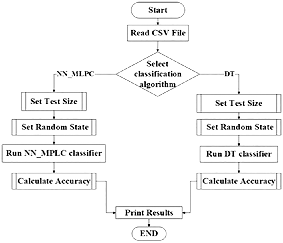
Figure 1: General flow chart

To discriminate between benign and malware files, this work grouped different tools to work as a system under security title.

It is important to mention that the computer used in this work is ACER, with Intel CORETM i7–7500 U, 2.7 GHz with TURBO Boost up to 3500. With NVIDIA GeForce MX130 with 2 GB VRAM. The computer employs an 8 GB DDR3 L Memory.

6  Work Methodology-Subgrouping Method

Studying the collected data from previous work was necessary to differentiate useful data from other data.

Accordingly, it was necessary to indicate what number of features produced maximum accuracy, good accuracy, or low accuracy so that indicators can be defined for the subgrouping method. According to previous observations and results obtained, it is possible to define three levels of accuracy as seen by the researchers:

A) High accuracy: in NN_MLPC, 0.97 considered as high accuracy and maximum accuracy obtained was within this range.In Decision Tree, things are different, DT gave accuracies within 0.97 in many cases, but also gave an accuracy within 0.98 in many other cases. So, in DT 0.97 and 0.98 will be considered as high accuracy and both accuracies will be taken into consideration in this work

B) Good Accuracy: in NN_MLPC obtaining 0.95 and 0.96 considered as good accuracy.

C) Low Accuracy: starting from 0.94 and less can be considered as low accuracy since low number of runs produced such accuracy or less.In DT, 0.94 or less will be considered also as low accuracy in comparison with the number of runs that gave higher accuracies.

To avoid doing all the possible combinations of the 29 features, a smaller number of features is selected for each of the four types of runs, i.e., subgrouping the 29 features according to results obtained previously. For each type, the following algorithm is implemented.

1)   Define High accuracy, Good accuracy and Low accuracy ranges

2)   For each classification algorithm used i.e., NN_MLPC and DT and according to previous observations:

a)   Selecting the smallest number of features that produced an accuracy within the high accuracy. Creating a new set, lets name it set x.

b)   According to previous observations new several features were nominated to participate in the experiments.

c)   Do several run on set x, by replacing some features by others from the nominated features and keeping the number of features the same. Each run will include the replacement of one feature only.

d)   Adding more features from the nominated set of features, in steps and re-run the experiment.

e)   Using the nominated features, a replacement to the features in steps but keeping the number of features fixed. And re-run the experiment.

f)   Halting the process when the number of features reaches the number of features which produced the highest number of accuracy previously.

Deciding the number of features in these sets is made through studying the previous results, i.e., those sets of features that gave higher accuracy than others. The choice of exchange features is also based on the same idea.

The procedure is halted when the number of features used in a set reaches the number of features that gave maximum accuracy in previous work, since this number is sufficient. Tests were done for some types to add more features after reaching the number of features that gave the maximum accuracy; it was notable that accuracy decreased, sometimes the decrease was slight, but still, it is less than the maximum accuracy.

Implementation of the work required the following steps:

A) Creating the set of features in an independent .csv file, to prepare it to the run.

B) The .csv file is imported to the program.

C) Making runs for both algorithms using the two combinations of test_size and random_state. Totaling four runs for each csv file.

6.1 NN_MLPC_0.3_10

According to previous results in [4], twenty-one and twenty-eight features produced maximum accuracy. The start was with combinations of 11 features to observe accuracy obtained. The 11 features were chosen as a starting point because it produced accuracy of 0.97 which is considered to be in the high accuracy area. Results showed that using 15 features produced maximum accuracy, whereas in previous work using 21or 28 features produced the maximum accuracy.

Noting that for the NN_MLPC runs with combinations of 15, 21, 25 and 28 features were used in addition to the combinations of 11 features, also combinations with less than 11 features were tested to check their impact.

Taking these steps of number of features comes from the observations in previous work [4], 11 features was the number of features with which first 0.97 accuracy obtained, 15 features when more stable graph obtained, 21 and 28 features when the same maximum accuracy obtained, 25 features was a step in the middle to test since in other types 25 features obtained the highest accuracy. This is also applied to all the next types of each number selected depending on some observations.

6.2 NN_MLPC_0.15_3

According to previous results [4], twenty-three features produced maximum accuracy. So, the runs will include combinations of 23 features at most.

Using thirteen features, accuracy of 0.97 was obtained which considered as high accuracy [4]. Hence, in this case 13 features are used to start with.

Subsequent sets of runs included 15, 18, 20, 21, 22 and 23 features, to obtain the highest accuracy value.

6.3 DT_0.3_10

Previous results stated that six features attained an accuracy in the 0.97 [4], fourteen features to get inside 0.98 which is high accuracy and 25 features to obtain the maximum accuracy. A start was with combinations of 6 features then of 9 features. Subsequently, combinations of 14, 18 and 25 features were used.

6.4 DT_0.15_3

Five features to get 0.97 range, eight features to get into the 0.98 according to previous results [4]. Twenty-Seven features to obtain maximum accuracy. Starting with 5 features, through 6, 8, 9, 10, 15, 18, 20, 22 and 27 features; sets of runs were carried out.

Total number of runs in NN_MLPC were 77 runs. For DT were 70 runs.

In this work each type has a different number of runs and different added features. This is because observations from previous work were used as a guide for selecting the number of features each time. Each type produced different observations with different number of features, so, steps used in each type are different from the others.

7  Results

Bar charts are used in this work to present the results obtained. This type of charts is self-explanatory and gives a better understanding. The charts are meant to show the range of accuracies that were obtained in the runs for each type, each chart will show how in each case study the accuracy changes. Before drawing the chart, all the accuracies obtained from each run were sorted from the smallest value to the highest value. What will be shown in each chart is how a variation of accuracies is obtained with different case studies. Each case study represents a set of features and number of features. In all the types, the last case study represents the maximum accuracy and the number of features used to attain it.

Tab. A1 includes the names of each feature, in the next sections feature’s number according to Tab. A1 will be mentioned.

7.1 NN_MLPC_0.3_10

Fig. 2 shows the Bar chart for the runs of NN_MLPC_0.3_10. The following can be noticed:

A) Lowest accuracy obtained when features 19 to 29 (Tab. A1) were used, with accuracy within 0.79. Add to that, the good accuracy obtained was within 0.95 and high accuracy of 0.97, it was notable that using features between 20 to 29 only make the accuracy decrease to levels of 0.91 and 0.92.

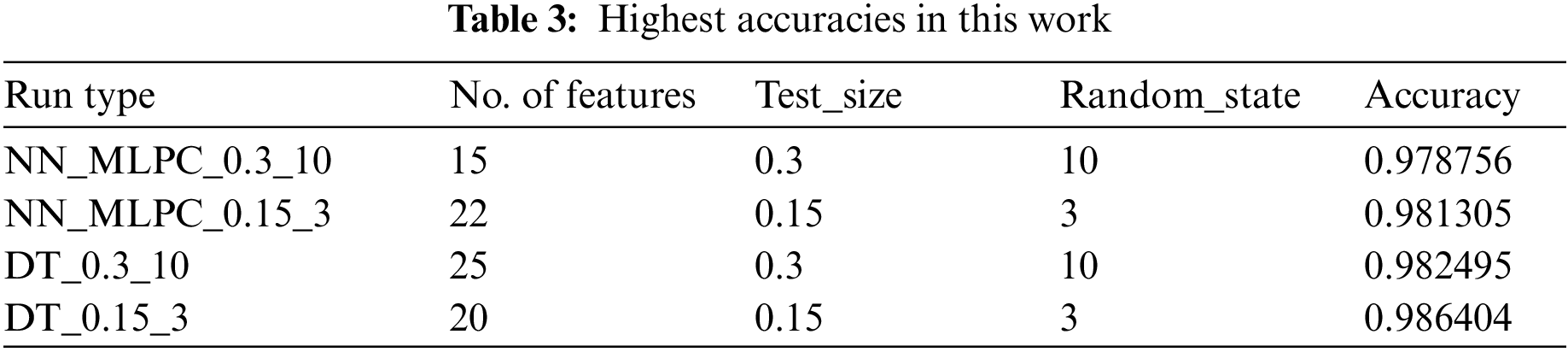
B) The maximum accuracy obtained was when using 15 features (0.97875595). Noting that 0.978 obtained also with 11 features, 21 features, 25 features and 28 features. But all the runs got a value less than the maximum value.

C) Using 11 features first 0.97 accuracy obtained. Not all the sets of 11 features produced an accuracy of 0.97. other combinations of 11 features produced the lowest accuracy, same thing is implied on sets of features higher than 11 features.

D) In [4], when 29 features are used 0.97790619 accuracy was obtained, but here, when subgroups from those 29 features are used a higher accuracy obtained, in many times, also, the same number of features brought a high accuracy sometimes and in other times, low accuracy.

As an example, in other run where 15 features are used, the accuracy obtained is: 0.95292318; whereas point B stated that when certain combination of 15 features is used, highest accuracy obtained.

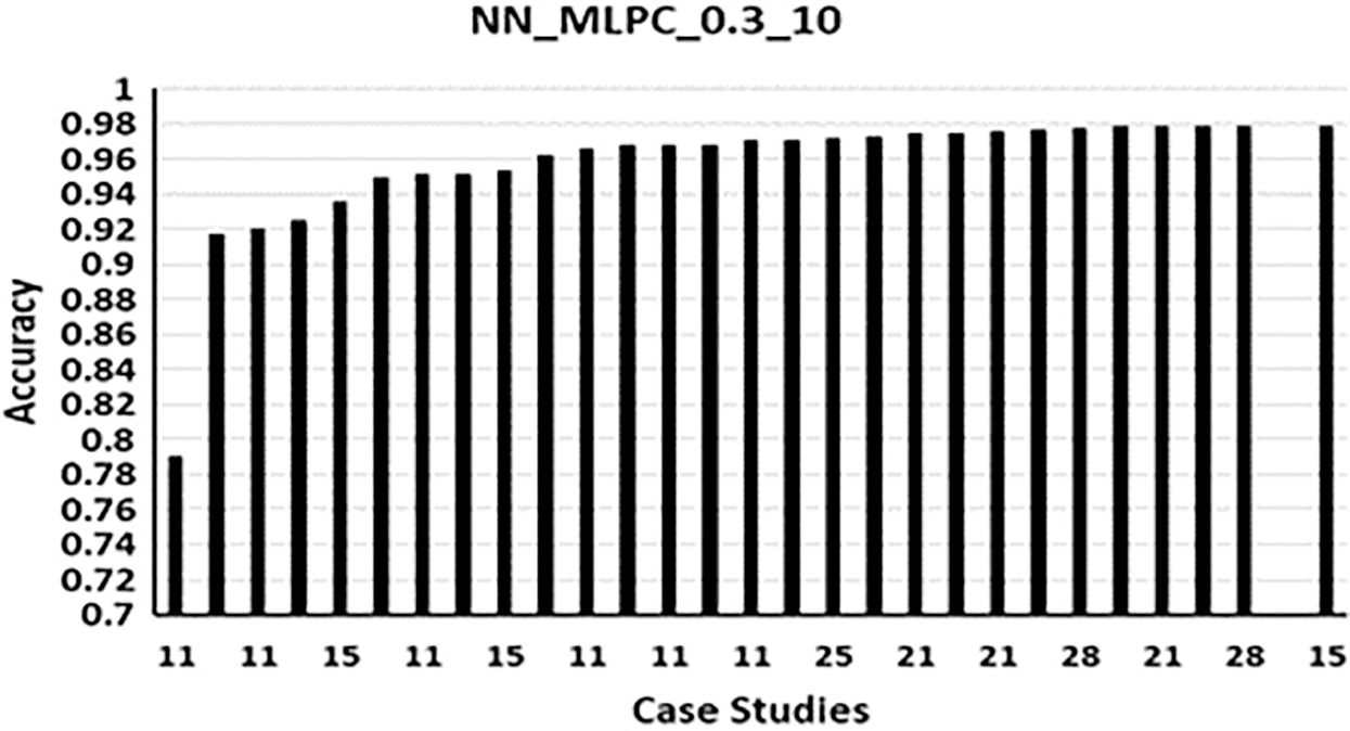
Figure 2: NN_MLPC_0.3_10

7.2 NN_MLPC_0.15_3

Fig. 3 shows the Bar chart for the runs of NN_0.15_3. The following can be noticed:

A) Lowest accuracy obtained using 15 features; 29 down to 15 (Tab. A1), the accuracy was: 0.91128484. Note that again using the last 10 features (feature 20 to feature 29) as most features led to lowest accuracy.

B) Highest accuracy obtained was: 0.98130523, using 22 features. It is the only run which gave an accuracy in the range of 0.98 between all the runs of NN_MLPC, other runs with 22 features produced a lower accuracy. Even in [4] obtained and accuracy of 0.976 as the maximum accuracy using 23 features.

C) Using 13 features the first 0.97 obtained, like the NN_MLPC_0.3_10 not all the combinations of 13 features produced the 0.97, the only one set of 13 features produced 0.97.

D) In general, if most features used from 20 to 29 a lower accuracy can be obtained, for example, when 13 features used (14 to 26) the accuracy obtained was 0.93847723, also, when 18 features were used 1 to 5 and 17 to 29, the accuracy obtained was 0.94323589, another example is when 23 features were used ten of them were 9 to 13 and 1 to 5, the remaining 13 features were 17 to 29, the accuracy obtained was 0.96057104.

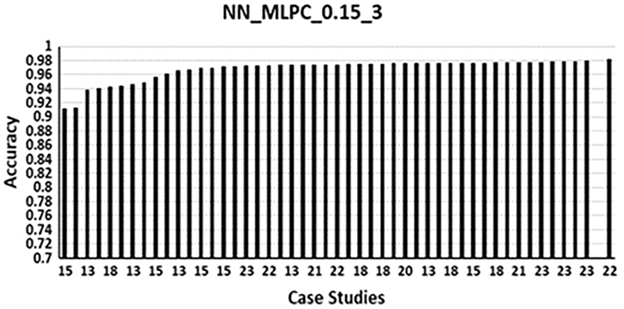
Figure 3: NN_MLPC_0.15_3

7.3 DT_0.3_10

Fig. 4 shows the bar chart for the runs of DT_0.3_10. The following can be noticed:

A) Lowest accuracy obtained using 6 features 20 to 25 (Tab. A1) the accuracy obtained was 0.75985724, note that again using only the features from the last 10 features in this case 20 to 25 resulted in lowest accuracy. To support this, using 9 features 21 to 29 an accuracy of 0.82545887 was obtained. This also was observed in NN_MLPC.

B) The highest accuracy obtained using 25 features, the accuracy obtained was 0.98249490. The second highest accuracy was 0.98164514, with 25 features.

C) The high accuracy was between 0.971 and 0.982. Accuracy of 0.971 was obtained using 6 features only. It can be shown that using 9 features a low accuracy obtained, but this was because the used features were selected between 20-to-29.

D) It was notable that 0.98 was repeated for many times. Starting from using 14 features, accuracy of 0.98113528 was obtained. Another 0.98 is obtained using different combination of 14 features which produced an accuracy of 0.98028552.

E) With 25 features an accuracy of 0.97824609 is obtained, while three runs before, one with 18 features and two with 22 features obtained an accuracy of 0.98.

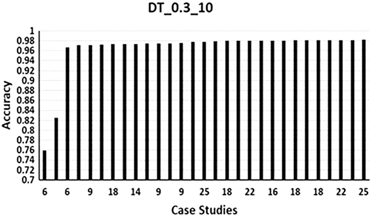
Figure 4: DT_0.3_10

7.4 DT_0.15_3

Fig. 5 shows the Bar chart for the runs of DT_0.15_3. The following can be noticed:

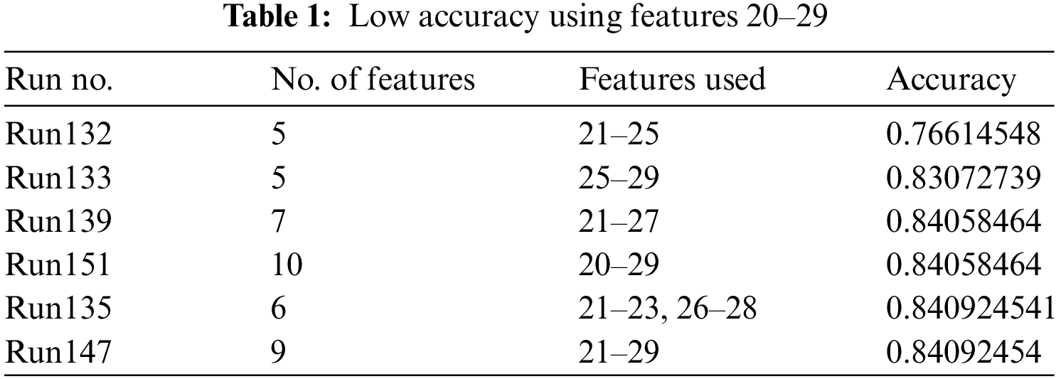
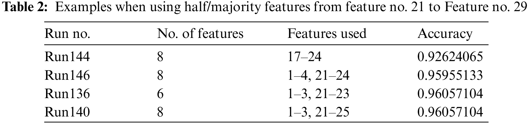
A) Lowest accuracy obtained with five features which are feature 21 to feature 25 (Tab. A1), the accuracy is 0.76614548, this was predictable since features used was between feature 20 to feature 29 only. Tab. 1 give some examples for low accuracy due to incorporating a whole of the set from the range 20 to 29. Also, Lower accuracy than normal obtained when including features starting from 20 to 29 as the majority features. Tab. 2 presents some of these examples.

B) Highest accuracy obtained was when using 20 features (1–7, 11–19 and 21–24 see Tab. A1) the accuracy was 0.98640381, this accuracy was the highest accuracy ever obtained between all the accuracies obtained in all cases in this work.

C) Only five features gave 0.97 accuracy. Eight features gave the first 0.98 level of accuracy. Also, 10, 15 and18 sets of features obtained 0.98. twenty features produced maximum accuracy.

D) Incorporating higher number of features does not reflect a high accuracy, for example, while eight features produced high accuracy like 0.98, increasing the number in many cases reduced the accuracy level.

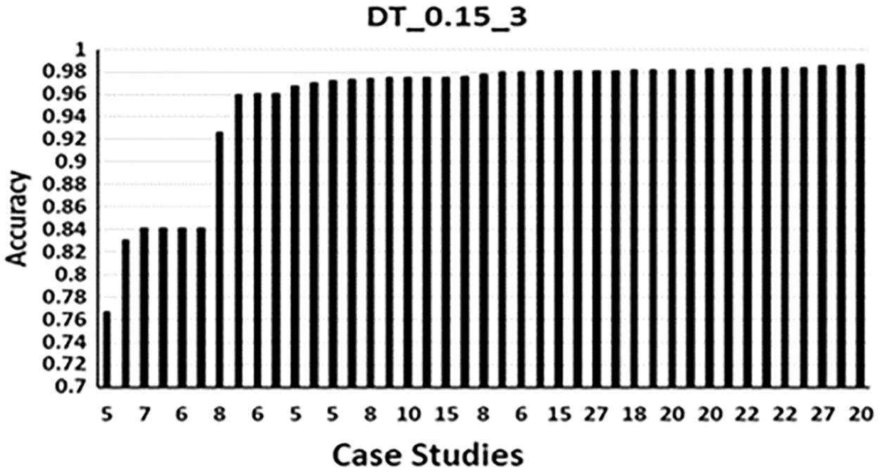
Figure 5: DT_0.15_3

To give an example of how the analysis for the results of this work is done; in addition to the charts in Fig. 2 through Fig. 5, two additional charts are presented in Figs. 6 and 7. Fig. 6 which is a combo chart that shows each run with its number of features used and corresponding accuracy for the NN_MLPC_0.15_3. The number of features is represented in the right axis and the accuracy represented in the left axis

Fig. 7 is a similar combo chart that shows each run with its accuracy and number of features for the DT_0.15_3.

Chose NN_MLPC_0.15_3 and DT_0.15_3 because these types produced the maximum accuracies in their classification algorithm. Figs. 6 and 7 show the variation of the accuracy obtained in each run using different sets of features. They are also show how the features used and their number affected the accuracy. The range of the y-axis is chosen to suit its own result values. The chart of NN_MLPC_0.15_3 accuracy axis started with 0.8 since the lowest accuracy obtained is 0.91 in this type. While the chart of DT_0.15_3 accuracy axis started with 0.7 since the lowest accuracy obtained is 0.76.

The charts show that the accuracy changes with the features used in the set but not the number of features. For example, in Fig. 6, there are several runs with 13 features, each run has a different value of accuracy depending on the specific features used. The same can be said about the other sets. This contribute to the thinking of the combination of used features would affect the accuracy, this idea is supported by the observation of the features 20 to 29 when they work together as a combination of features and work alone, or as most features within the set, accuracy becomes the lowest or at least low. While including one or two of them in other combination they may behave in a way that will enhance the accuracy, this was notable during the work implementation. Next section will show such cases.

Figure 6: NN_MLPC_0.15_3

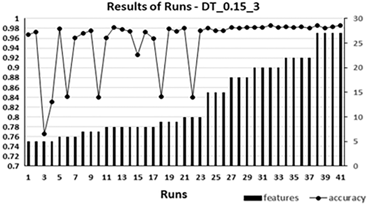
Figure 7: DT_0.15_3

8  Discussion

8.1 Work Observations

a. NN_MLPC

Observations in NN_MLPC_0.15_3 showed that using certain combination of 18 features got an accuracy of 0.9765, 20 features produced 0.976, other combination of 20 features produced 0.978, add to that 21 features gave 0.9769, 22 features gave 0.9786 and 23 features gave 0.9765, 0.978, 0.976 and 0.979, most of these results are better than the maximum accuracy given by previous implementations. Also, other combinations with the same number of features gave less accuracy even less than the good accuracy. This contributed to the importance of feature combinations used to produce an improved accuracy.

From what is mentioned in Section 7 (results) in NN_MLPC_0.3_10 and NN_MLPC_0.15_3 point C in addition to what was obtained from previous implementations, the first 0.97 is obtained using 11 features for NN_MLPC_0.3_10 and 13 features in NN_MLPC_0.15_3. This means that there is a need to use at least 11 features to get such accuracy in NN_MLPC_0.3_10 and 13 features in NN_MLPC_0.15_3, this contributes to the question about the impact of the number of features used on accuracy. This is applied also to all the remaining types. Each type required a different number of features to get a good accuracy.

Obtaining an accuracy less than 0.97 when using less than eleven or thirteen features for both types indicates that the number of features used in these cases is an important factor. However, not all features have a positive contribution to increase the accuracy. Features required to improve the accuracy need to be recognized, even with the same number of features.

Maximum accuracy obtained in NN_MLPC was 0.9813 when using 22 features in NN_MLPC_0.15_3, noting that this was the only set with this number that gave the maximum accuracy. Other sets with the same number of features gave lower values of accuracy. This shows the importance of finding the correct combination that must be used; note that this was the only combination of features which produced an accuracy in the range of 0.98, all previous implementations did not obtain such accuracy. This also applies to NN_MLPC_0.3_10 type.

b. Decision Tree (DT)

Tab. 2 shows that in Run130, features 6 to 10 are used, using 5 features only, made the accuracy to be lower than good. This emphasizes the importance of the number of features used. It is true that 0.97 was obtained using 5 features, but 0.97 in this case was not in the maximum accuracy range for DT. Low accuracy results were also obtained with NN_MLPC when the number of features is small.

c. General Observations

The results showed that with DT using 5 or 6 features 0.97 range of accuracy was obtained, while in NN_MLPC using 11 features in NN_MLPC_0.3_10 and 13 features in NN_MLPC_0.15_3 gave the 0.97 accuracy. All statistics in DT are different from the NN_MLPC. However, the common facts found in both algorithms are those related to answering the questions on the effects of the number of features, the specific features used and the combinations of features.

In both algorithms and runs implemented, features 20 to 29 reduced the accuracy when they were used alone or as a majority in a bigger set. On the other hand, in more than one situation individual features, small sets or maybe the whole range from the range showed positive impact on accuracy when they are included in a larger set of other ranges. For example, when feature number 26 was included in one of the cases, highest accuracy was obtained, other cases showed positive contributions of individual features from 20 to 29. But in general, using majority or all the features from this range showed bad accuracies.

It is important to emphasize here that including features from 20–29 will behave differently if they were included in a bigger set of features, it was notable that many results in the range of highest accuracy was obtained when including some or even all the 20 to 29 features, but this was in runs when the number of features is high and the features used from the ranges 1 to 10 and 11 to 19 is bigger. This can be observed in Section 7 Tab. 2 which presents examples of lower level of accuracies due to incorporating high percentage from the features 21 to 29.

The results also showed that several individual features improve the accuracy. Some sets of features when included within larger sets have a positive impact on the accuracy in both NN_MLPC and DT. At the same time, the effect of these sets is different between NN_MLPC and DT. In general, these sets have the best impact, the difference between the two algorithms is what features to add with these sets to obtain the best accuracy.

Accordingly, it can be thought that some individual features or sets of features may take the role of positive impact whatever the algorithm.

In both algorithms, entering the region of high accuracy appeared with certain feature numbers; however, other features need to be added to get the highest accuracy.

Tab. 3 shows the maximum accuracies obtained for the two algorithms.

8.2 Comparison with Previous Work

Starting with the procedure used in this work, subgrouping the feature for testing is the way that this work implemented to reach the highest accuracy with a smaller number of runs and a lower time cost. Other implementations used other strategies discussed in the Related Work section. The procedure used in this work showed the improved performance to obtain answers to the questions mentioned previously. For the numerical part of the results, what is obtained was more, the same, or slightly less than the results obtained in previous implementations. For example, in NN_MLPC, enhanced results were obtained. And in DT a slightly fewer results were obtained. The most important thing that this way obtained the required results.

Previous implementations used different strategies to collect and study the portable executable features, got good accuracies. Features used in those previous works were the features collected in this work.

Tab. 4 will compare results obtained in this work with the results obtained in previous work of [4], then a comparison is made for the numerical results obtained in other previous works.

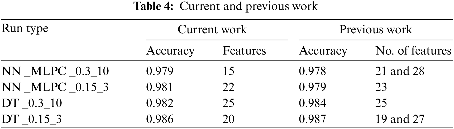
Tab. 4 showed that for NN_MLPC an enhanced accuracy is obtained in this work. Also, fewer features are used to attain highest accuracy. With NN_MLPC_0.3_10, features used were 15 while in [4], 21 or 28 features were needed to get less than what is obtained in the current work. This proves that the combination of the features affects the accuracy since, in the current work, other combinations of 15 features up to 28 features were used, but accuracies obtained were less than or even much lower. So, number of features, features used and combination of these features are proved to affect the accuracy. It showed that also high number of feature does not mean high accuracy.

For DT_0.15_3 Tab. 4 showed that accuracies obtained in [4] are slightly better, but number of features in DT_0.3_10 is the same in both works taking into consideration that the difference between the previous work and this work is that previous work included the feature number 25 in the set, in this work the feature 25 is replaced by the feature 26. Since results are better in previous work then feature 26 gave a negative effect or no effect in this run of the current work, or in other words in this combination of features, since previously in other situation it is mentioned that including feature 26 in the set brought the highest accuracy, so, this combination will work better if the feature 25 is included instead of the feature 26.

In DT_0.15_3, 20 features used in the current work gave an accuracy less by 0.001, while using 19 or 27 features in [4] gave an accuracy more than the current work’s accuracy with 0.001.

According to Tab. A1, if the collection of features used in this work is divided into three sets, one to ten, eleven to twenty and twenty-one to twenty-nine, then, it will be notable that all the high accuracies obtained contains features from the three sets. Other accuracies were low; they also contain features from the three sets. Tab. 5 will list a sample of the runs done in NN_MLPC and DT with the accuracies obtained and features used.

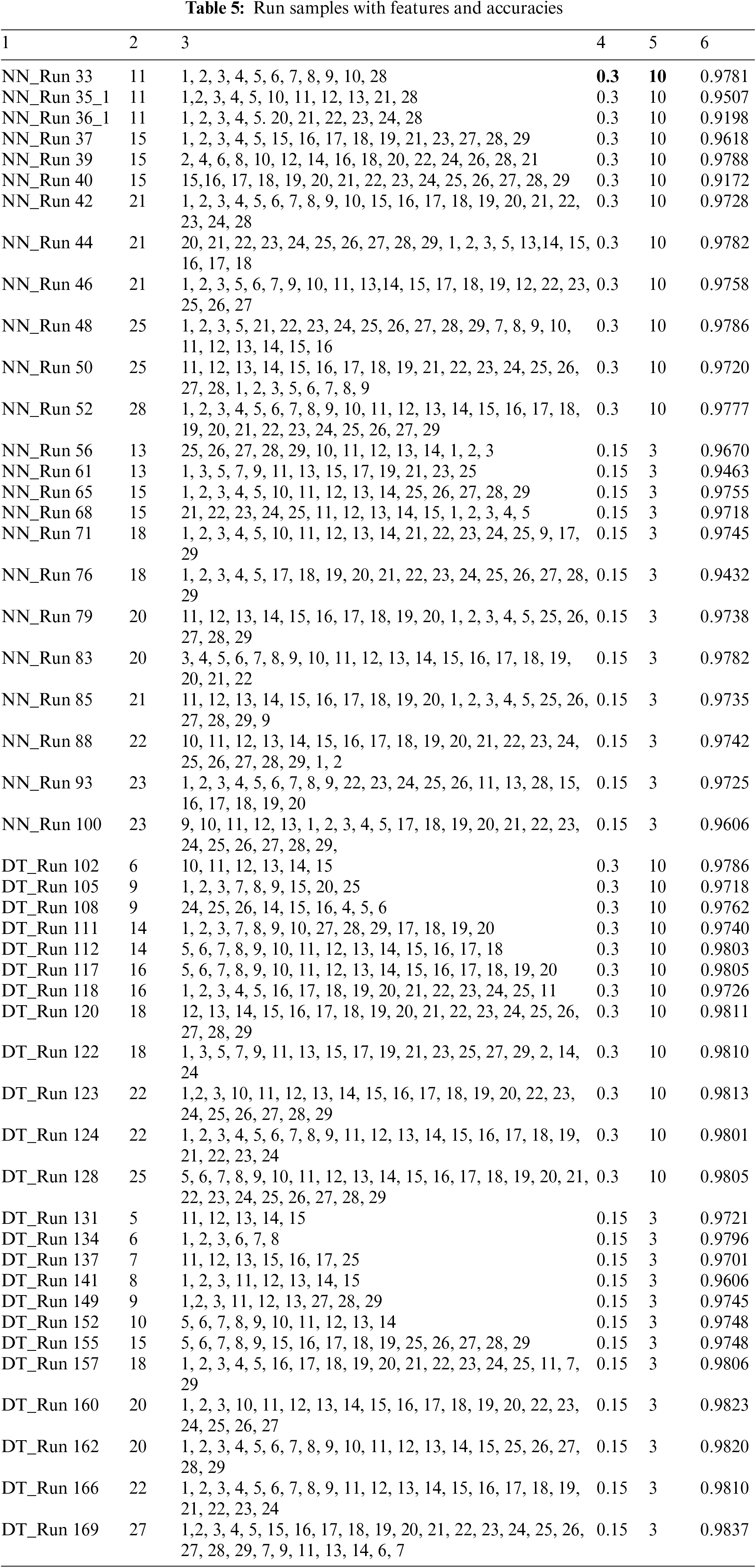
It can be noticed in Tab. 5 that some values of accuracy were obtained which are near the maximum accuracy in both types. But the aim was to find a number and combination which produce a high accuracy. The maximum accuracy obtained using this technique with a smaller number of features.

Accuracies of 98% and 97% were attained in [3], no fractions announced by the work, for current work same range of accuracies were obtained in DT only, since [3] implemented only DT and other algorithms, NN_MLPC was not used, the current work attained an accuracy of 98.6% with DT; comparing this accuracy with the 98.26% obtained in [20] using DT, it is also higher.

Column names of Tab. 5:

1.    NN or DT and Run Number: where NN stands for NN_MLPC. DT stands for Decision Tree. NN_Run No. which stands for NN_MLPC with run number, or DT_Run No. for DT and the run number

2.    Number of features

3.    Features Used

4.    Test_Size

5.    Random_State

6.    Accuracy obtained.

9  Conclusions

Researchers in previous works stated their strategies and plans to study Portable Executable files, selecting the features to be used, some of the researchers made their studies on packed files, but still the features of PE file played the main role in distinguishing benign from malicious files.

Twenty-nine features were used in the study, which were previously collected in other work and studied them using subgrouping method to observe the accuracy each time. An independent data set were prepared and saved for each run.

Two classification algorithms were used NN_MLPC and DT. Four types of runs were carried out, NN_MLPC_0.3_10, NN_MLPC_0.15_3, DT_0.3_10 and DT_0.15_3. The numbers included in each type represents the test_size and random_state, respectively.

Results obtained from this work has practical part and numerical part. Practical part was the observations and the inferences which is summarized with the factors impacting the accuracy of malware detection, those factors are the number of features used, the features included and the combination of features used. For the numerical results accuracies of 0.979 and 0.981 for NN_MLPC. As for DT 0.9825 and 0.986 were obtained.

The results obtained in this work was an enhanced result sometimes and equals or slightly less than previous work other time, this was the main aim of the work, when a slightly less accuracy obtained means that there is certain impact of the features on the accuracy, so those features can be studied more or be taken into consideration in future to not include them since their effect were negative.

The process of subgrouping showed its high efficiency comparing to previous implementations; using certain subsets of features in steps according to previous observations till obtaining the highest accuracy can reduce the time and produce good results.

In this work, it was shown that the number of features used, the specific features included and the combination of features play the major role in accuracy. Thus, using a high number of features is not sufficient by itself to obtain high accuracy, add to that high number of features may lead to fall into the curse of dimensionality problem.

For the future work, according to the enhanced results obtained in this work, a deeper study to the features with different methodology can be carried out, also, incorporating more features to see their impact on accuracy. The idea includes employing more performance measurements metrics like sensitivity, specificity, precision, f_measure and/or G-mean.

Acknowledgement: My gratitude and thanks to Dr. Harith J. Al-Khshali (my father), who helped and supported me in this work, unfortunately, he passed away before completing the final versions of the work, it is a big loss to the science.

Funding Statement: The authors received no specific funding for this study.

Conflicts of Interest: The authors declare that they have no conflicts of interest to report regarding the present study.

Appendix A

Tab. A1 contains the feature numbers and names in this work.

References

1. J. Bai, J. Wang and G. Zou, “A malware detection scheme based on mining format information,” The Scientific World Journal, vol. 2014, Article ID 260905, pp. 11, Hindawi Publishing Corporation, 2014. https://doi.org/10.1155/2014/260905. [Google Scholar]
2. Y. Liao, “PE-Header-based malware study and detection,” Computer Science, pp. 4, Corpus ID: 16132156.2012, Retrieved from the University of Georgia, 2012. [Google Scholar]
3. A. Kumara, K. S. Kuppusamya and G. Aghilab, “A learning model to detect maliciousness of portable executable using integrated feature set,” Journal of King Saud University-Computer and Information Sciences, vol. 31, no. 2, pp. 252–265, Publisher: Elsevier, 2019. [Google Scholar]
4. H. H. Al-Khshali, M. Ilyas and O. N. Ucan, “Effect of PE file header features on accuracy,” in 2020 IEEE Symp. Series on Computational Intelligence (SSCI), Canberra, ACT, Australia, Published in IEEE Xplore, pp. 1115–1120, 2020. [Google Scholar]
5. J. Gupta and J. Singh, “Detecting anomaly based network intrusion using feature extraction and classification techniques,” International Journal of Advanced Research in Computer Science, vol. 8, no. 5, pp. 1353–1356, ISSN No. 0976-5697. 2017. [Google Scholar]
6. H. El Merabet and A. Hajraoui, “A survey of malware detection techniques based on machine learning,” International Journal of Advanced Computer Science and Applications (IJACSA), vol. 10, no. 1, pp. 366–373, 2019. [Google Scholar]
7. A. Kumar and G. Aghila, “Portable executable scoring What is your malicious score?,” in Int. Conf. on Science, Engineering and Management Research (ICSEMR 2014), Chennai, India, pp. 1–5, 2014. [Google Scholar]
8. L. Binxiang, Z. Gang and S. Ruoying, “A deep reinforcement learning malware detection method based on PE feature distribution,” in 6th Int. Conf. on Information Science and Control Engineering (ICISCE), Shanghai, China, pp. 23–27, 2019. [Google Scholar]
9. T. Rezaei and A. Hamze, “An efficient approach for malware detection using PE header specifications,” in 6th Int. Conf. on Web Research (ICWR), Tehran, Iran, pp. 234–239, 2020. [Google Scholar]
10. T. Wang, C. Wu and C. Hsieh, “Detecting unknown malicious executables using portable executable headers,” in Fifth Int. Joint Conf. on INC, IMS and IDC, Seoul, Korea (Southpp. 278–284, 2009. [Google Scholar]
11. T. Wang and C. Wu, “Detection of packed executables using support vector machines,” in Proc. of the 2011 Int. Conf. on Machine Learning and Cybernetics, Guilin, China, pp. 717–722, 2011. [Google Scholar]
12. V. Visoottiviseth, P. Sakarin, J. Thongwilai and T. Choobanjong, “Signature-based and behavior-based attack detection with machine learning for home IoT devices,” in 2020 IEEE Region 10 Conf. (TENCON), Osaka, Japan, pp. 829–834, 2020. [Google Scholar]
13. M. R. Islam, A. W. Naji, A. A. Zaidan and B. B. Zaidan, “New system for secure cover file of hidden data in the image page within executable file using statistical steganography techniques,” International Journal of Computer Science and Information Security (IJCSIS), vol. 7, no. 1, pp. 273–279, 2009. [Google Scholar]
14. J. Clark and S. Banik, “Building contemporary and efficient static models for malware detection,” in 2020 IEEE SoutheastCon, Raleigh, NC, USA, pp. 1–6, 2020. [Google Scholar]
15. D. Devi and S. Nandi, “PE file features in detection of packed executables,” International Journal of Computer Theory and Engineering, vol. 4, no. 3, pp. 476–478, Publisher: IACSIT Press, 2012. [Google Scholar]
16. M. Zakeri, F. F. Daneshgar and M. Abbaspour, “A static heuristic approach to detecting malware targets,” Security and Communication Networks, vol. 8, no. 17, pp. 3015–3027, Publisher: John Wiley & Sons, Ltd, 2015. [Google Scholar]
17. I. Indre and C. Lemnaru, “Detection and prevention system against cyber-attacks and botnet malware for information systems and internet of things,” in 2016 IEEE 12th Int. Conf. on Intelligent Computer Communication and Processing (ICCP), Cluj-Napoca, Romania, pp. 175–182, 2016. [Google Scholar]
18. E. Raff, J. Sylvester and C. Nicholas, “Learning the PE header, malware detection with minimal domain knowledge,” in Proc. of the 10th ACM Workshop on Artificial Intelligence and Security (2017), Dallas, TX, USA, pp. 121–132, 2017. https://doi.org/10.1145/3128572.3140442. [Google Scholar]
19. N. T. Vu. and D. H. Le, “A virus detection model using portable executable feature extraction,” Preprints Journal, pp. 7, Publisher MDPI AG, 2019. [Google Scholar]
20. N. Maleki, M. Bateni and H. Rastegari, “An improved method for packed malware detection using PE header and section table information,” I.J. Computer Network and Information Security, vol. 11, no. 9, pp. 9–17, Published Online September 2019 in MECS, 2019. [Google Scholar]
21. Z. Fuyong and Z. Tiezhu, “Malware detection and classification based on N-grams attribute similarity,” in 2017 IEEE Int. Conf. on Computational Science and Engineering (CSE) and IEEE Int. Conf. on Embedded and Ubiquitous Computing (EUC), Guangzhou, China, vol. 1, pp. 793–796, 2017. [Google Scholar]
22. S. Jophin, M. Vijayan and S. Dija, “Detecting forensically relevant information from PE executables,” in 2013 Third Int. Conf. on Recent Trends in Information Technology (ICRTIT), Chennai, India, IEEE, pp. 277–282, 2013. [Google Scholar]
23. A. P. Namanya, Q. K. A. Mirza, H. Al-Mohannadi, I. U. Awan and J. F. P. Disso, “Detection of malicious portable executables using evidence combinational theory with fuzzy hashing,” in 2016 IEEE 4th Int. Conf. on Future Internet of Things and Cloud, Vienna, Austria, pp. 91–98, 2016. [Google Scholar]
24. M. S. Yousaf, M. H. Durad and M. Ismail, “Implementation of portable executable file analysis framework (PEFAF),” in Proc. of 2019 16th Int. Bhurban Conf. on Applied Sciences & Technology (IBCAST), Islamabad, Pakistan, pp. 671–675, 2019. [Google Scholar]
25. A. M. Radwan, “Machine learning techniques to detect maliciousness of portable executable files,” in Int. Conf. on Promising Electronic Technologies (ICPET), Gaza, Palestine, pp. 86–90, 2019. [Google Scholar]
26. V. Atluri, “Malware classification of portable executables using tree-based ensemble machine learning,” in IEEE Southeastcon, Huntsville, AL, USA, pp. 1–6, 2019. [Google Scholar]
27. B. B. Rad, M. Masrom and S. Ibrahim, “Opcodes histogram for classifying metamorphic portable executables malware,” in 2012 Int. Conf. on E-Learning and E-Technologies in Education (ICEEE), Lodz, Poland, pp. 209–213, 2012. [Google Scholar]
28. M. U. M. Saeed, D. Lindskog, P. Zavarsky and R. Ruhl, “Two techniques for detecting packed portable executable files,” in Int. Conf. on Information Society (i-Society 2013), Toronto, ON, Canada, IEEE Xplore, pp. 22–26, 2013. [Google Scholar]
29. F. H. Ramadhan, V. Suryani and S. Mandala, “Analysis study of malware classification portable executable using hybrid machine learning,” in 2021 Int. Conf. on Intelligent Cybernetics Technology & Applications (ICICyTA), Bandung, Indonesia, pp. 86– 91, 2021. [Google Scholar]
30. H. Kim and T. Lee, “Research on autoencdoer technology for malware feature purification,” in 21st ACIS Int. Winter Conf. on Software Engineering, Artificial Intelligence, Networking and Parallel/Distributed Computing (SNPD-Winter), Ho Chi Minh City, Vietnam, pp. 236–239, 2021. [Google Scholar]
31. J. A. Diaz and A. Bandala, “Portable executable malware classifier using long short term memory and sophos-reversinglabs 20 million dataset,” in TENCON, 2021-2021 IEEE Region 10 Conf. (TENCON), Auckland, New Zealand, pp. 881–884, 2021. [Google Scholar]
32. F. Manavi and A. Hamzeh, “Static detection of ransomware using LSTM network and PE header,” in 26th Int. Computer Conf., Computer Society, Tehran, Iran, pp. 1–5, 2021. [Google Scholar]
33. W. Zheng and K. Omote, “Robust detection model for portable execution malware,” in ICC 2021–IEEE Int. Conf. on Communications, Montreal, QC, Canada, pp. 1–6, 2021. [Google Scholar]
34. D. Demirci, N. Sahin, M. Sirlanci and C. Acarturk, “Static malware detection using stacked BiLSTM and GPT-2,” IEEE Access, vol. 10, pp. 58488–58502, 2022. [Google Scholar]
35. Y. Gao, H. Hasegawa, Y. Yamaguchi and H. Shimada, “Malware detection using lightGBM with a custom logistic loss function,” IEEE Access, vol. 10, pp. 47792–47804, 2022. [Google Scholar]
36. F. Zatloukal and J. Znoj, “Malware detection based on multiple PE headers identification and optimization for specific types of files,” 2017 Journal of Advanced Engineering and Computation (JAEC), vol. 1, no. 2, pp. 153–161, 2017. [Google Scholar]
37. A. Parisi, “Malware threat detection,” in Hands-on Artificial Intelligence for Cybersecurity. Implement Smart AI Systems for Preventing Cyber-Attacks and Detecting Threats and Network Anomalies, 1st ed., Birmingham, B3 2PB, UK: Packt Publishing, pp. 82, 2019. [Google Scholar]
38. E. Carrera, “Benign and malicious PE Files dataset for malware detection,” Data Set obtained from the following site: https://www.kaggle.com/amauricio/pe-files-malwares/data. And the License to use this Data Set can be found at. Available: https://creativecommons.org/publicdomain/zero/1.0/. 2018. [Google Scholar]
39. P. Josh, “Artificial neural networks,” in Artificial Intelligence with Python. A Comprehensive Guide to Building Intelligent Apps for Python Beginners and Developers, 1st ed., Birmingham, B3 2PB, UK: Packt Publishing Ltd, pp. 363, 2017. [Google Scholar]
40. A. A. Zaidan, B. B. Zaidan and F. Othman, “New technique of hidden data in PE-file with in unused area one,” International Journal of Computer and Electrical Engineering, vol. 1, no. 5, pp. 1793–8163, 2009. [Google Scholar]
41. S. Mihajlović, A. Kupusinac, D. Ivetić and I. Berković, “The use of python in the field of artificial intelligence,” in Int. Conf. on Information Technology and Development of Education–ITRO 2020, Zrenjanin, Republic of Serbia, 2020. [Google Scholar]