
 Submit a Paper
 Propose a Special lssue
 Open Access
ARTICLE
Performance Enhancement of Adaptive Neural Networks Based on Learning Rate
1 Department of Computer Science, Aligarh Muslim University, Aligarh, 202002, Uttar Pradesh, India
2 Department of Information Technology, Bhagwan Parshuram Institute of Technology (BPIT), GGSIPU, New Delhi, 110089, India
3 Department of Computer Science and Engineering, Maharaja Agrasen Institute of Technology (MAIT), GGSIPU, New Delhi, India
4 Department of Electrical Engineering, College of Engineering, Princess Nourah bint Abdulrahman University, P.O.Box 84428, Riyadh, 11671, Saudi Arabia
* Corresponding Author: Shabana Urooj. Email:
Computers, Materials & Continua 2023, 74(1), 2005-2019. https://doi.org/10.32604/cmc.2023.031481
Received 19 April 2022; Accepted 15 June 2022; Issue published 22 September 2022
 View Full Text
 Download PDF
Abstract
Deep learning is the process of determining parameters that reduce the cost function derived from the dataset. The optimization in neural networks at the time is known as the optimal parameters. To solve optimization, it initialize the parameters during the optimization process. There should be no variation in the cost function parameters at the global minimum. The momentum technique is a parameters optimization approach; however, it has difficulties stopping the parameter when the cost function value fulfills the global minimum (non-stop problem). Moreover, existing approaches use techniques; the learning rate is reduced during the iteration period. These techniques are monotonically reducing at a steady rate over time; our goal is to make the learning rate parameters. We present a method for determining the best parameters that adjust the learning rate in response to the cost function value. As a result, after the cost function has been optimized, the process of the rate Schedule is complete. This approach is shown to ensure convergence to the optimal parameters. This indicates that our strategy minimizes the cost function (or effective learning). The momentum approach is used in the proposed method. To solve the Momentum approach non-stop problem, we use the cost function of the parameter in our proposed method. As a result, this learning technique reduces the quantity of the parameter due to the impact of the cost function parameter. To verify that the learning works to test the strategy, we employed proof of convergence and empirical tests using current methods and the results are obtained using Python.Keywords
The cost function formed by an artificial neural network (ANN) is identified using the learning data to achieve artificial intelligence (A.I.) by describing the cost function created by an ANN. The parameters to make this cost function as minimal, to put it another way, A.I. learning is the cost procedure for optimizing a process; as a result, A.I. learning faces two challenges: The cost function description and its optimization is the first issue is the definition of the term the more data the ANN structure, the higher the cost function. As a result, the cost function has become more complicated [1,2] because the cost function parameter of local minimums increases [3]. As a result, the cost function first-order derivative is zero, called the local minimum. As a result, if A.I. learning is not done at this local minimum; as a result, the local minimum when only a small portion of the cost function rises, A.I. learning gets increasing in the amount of data required to make use of additional parameters. A.I. grows, the amount of data available. The ANN structure becomes difficult to increase. A.I. learning should be carried out with the help of the cost function with a lot of local minimums. The second challenge emerges when the optimization problem is handled for multiple local minima in a cost function [4–7]. The major goal of a cost function with several local minimums is used in deep learning. The researcher added the complete parameter; the cost function first-order derivative is used Momentum based on the global minimum. As a result, the mathematical Lagrangian technique [8,9] is applied. The momentum approach [10,11] is also the available method based on the cost function first derivative. The first derivative is the result of parameter learning being performed by the increased model parameters. As a result, even when the cost function first derivatives are zero, learning can proceed at a local minimum depending on the cost function first derivative, which was previously added. The cost function’s first derivative has been added; learning does not stop while it progresses; after it has done, you won’t have learned as much as you could have to be able; methods for solving this problem include changing the learning rate and adding an extra step Adaptive properties have been created for the momentum approach. This is an academic paper built on the momentum approach with the addition of an adaptive attribute, which is a step in the magnitude of the cost function changes with its parameter. The momentum method builds a step size based on the cost function, close to a feasible cost function with minimal value. In the text, more particular ideas and methodologies are covered in depth. The convergence of the parameters is defined in this method.
Since the introduction of machine learning, Artificial Neural Networks (ANN) have been on a meteoric rise [12]. Emerging neural architectures, training procedures, and huge data collectors continually push the state-of-the-art in many applications in deep learning of complex models. These are now partially attributed to rapid developments in these techniques and hardware technology. However, the study of ANN basics does not follow the same networks [13]; one of the most common ANN architectures for the Computer model is a lack of comprehension of its essential details [14] because of certain intriguing unexplainable phenomena to be noticed. Experiments have demonstrated that minor input changes can significantly impact performance, a phenomenon known as adversarial examples [15]. It is feasible to make representations that are completely unidentifiable, but convolutional networks strongly believe there are things. These instabilities constrain research on neural network operation and network improvements, such as enhanced neuron initialization, building architecture search, and fitting processes. Improved understanding of their qualities will contribute to Artificial Intelligence (A.I.) [16] and more reliable and accurate models. As a result, one of the most recent subjects area, how ANN work, which also has evolved into proper multidisciplinary research bringing together computer programmers, researchers, biologists, mathematicians, and physicists. Some strange ANN behaviors are consistent with complicated systems, which have been typically nonlinear, challenging to predict, and sensitive to small perturbations. Complex Networks (C.N.) main purpose is to examine massive networks produced from the neural network, complicated processes, and how they relate to different neural networks, such as biological networks. Its presence of the small-world C.N. phenomenon, for example, has been demonstrated in the neural network of the Caenorhabditis elegans worm [17]. Following discovered of similar topological characteristics in human brain networks, such as encephalography recordings [18], cortical connections analyses [19], and the medial reticular development of the brain stem [20]. The original gradient descent algorithm has been improved in several ways. Adding a “momentum” term to the update rule, as well as “adaptive gradient” methods like Adam and RMSProp [21,22], which combines RMSProp [23] with AdaGrad [24], are examples. Deep neural networks have used these strategies extensively.
There has recently been a lot of research into new strategies to adapt the learning rate. Academic and intuitive empirical support these claims [25]. These efforts rely on non-monotonic learning rates and support the idea of cyclical learning rates. Our proposed method produces a momentum learning rate. Recent theoretical work has shown that stochastic gradient descent is sufficient to optimize over-parameterized neural networks while making minimal assumptions. We aim to find an optimal learning rate analytically, rejecting the concept that only tiny learning rates should be employed, and then demonstrate the correctness of our statements experimentally. It is essential to automatically calculate the step size in gradient-based optimization based on the loss gradient that shows how each unknown parameter approaches convergence. Adaptive rate scheduling based on parameters such as RMSprop, Adam, and AdaGrad [26] has been created to achieve this goal and ensure that the method converges quickly in practice.
3 Methodology of Machine Learning
The AdaGrad method excessive accumulation of the RMSProp [27], and the cumulative squares of gradients method recommends just accumulating work for the most recent gradients [28].
where
Momentum and RMSProp are combined in the Adam algorithm [30]. For each parameter, Adaptive learning rates are also calculated using this algorithm. Like Momentum, RMSprop, and Adam preserves the previous gradient squares exponentially decaying average U, and Momentum keeps an exponential decay average of the earlier gradients m. The following is the Adam algorithm equation:
4 The Momentum Method and the Optimization Problem
The cost function was created using the learning data. The input data
4.1 Problem of the Optimization
To satisfy
whereas the number of learning data l and the optimization problem is as follows:
Gradient-based approaches are commonly employed to address the optimization problem Eq.(7) [31,32].
To discover parameter w, gradient-based approaches are utilized to ensure that perhaps the cost function gradient is zero. However, c(w) is not a convex cost function. Reducing the gradient to zero might be ineffective if c(w) is not a convex cost function. As a result, to improve learning performance, we used the Lagrange multiplier technique to recognize E(w) and identify the parameter w, which makes E(w) zero.
μ is a minor constant in this equation; an iterative parameter modification was utilized, a strategy to get w to satisfy Eq. (8) by resulting in zero.
The learning rate is defined as α, where α is a constant. The momentum approach is identical to Eq. (9).
The momentum technique is used to solve E(w) = 0.
mi=
Our methodology is based on the method of Momentum, which terminates learning when it reaches the cost function global minimum value, which is the point at which learning is well implemented. The following results can be obtained by modifying the learning rate:
Where
where ρ0 is constant, and Ui=
Lemma 1. The following is the relationship between mi and Ui:
Proof. [33] is where you’ll find the proof.
Eq. (10) gives us the following result when we use the relationship between mi and Ui:
Because
As a result, when the series μi converges to zero, the sequence wi also converges.
Theorem 1. It is necessary to identify the parameter that minimizes the cost function c. Our generated sequence {wi} limit value is a sequence with zero value for the cost function c. The relation between
Proof. Using the Taylor theorem with a sufficiently high number τ and a reasonably small value ρi, the appropriate calculation is performed:
where the second order is represented by part of o(wi+1- wi)2 is ignored. We can deduce the following from Eqs. (10) and (13):
As
As a result, we can acquire
Where δ = supremum-i>τ
It is possible that δ is smaller than 1 in Theorem (1). As a result, we explain why δ is smaller than 1 in further detail in the following corollary.
Corollary 1. The value of δ, is less than 1 as defined in Theorem (1).
Proof. To begin with, i is supposed to be derived from a number following a suitably large integer, τ.
Under the supposition that ρi and
is broken down into three pieces and calculated as follows:
and
Eqs. (14) and (15) produce a simple estimate, a cost function condition (c < 1), and μ. Eq. (16) should be shown to be less than 1, and from the definition of mi. Because
If sign
5.1 Experimental Results and Discussion
This paper compares GD, Adagrad, and Adam, our proposed technique, since our strategy’s momentum concept contains the momentum method influence. The performance of each method was examined in Sections 6.1 and 6.2 by supposing; that the cost functions are indeed two-variable functions. It is a visual representation of how the technology changes each parameter. We explored the problem in Section 6.3. Human-written0 to 9 numbers are classified. A dataset is the most fundamental data set to compare the performance of deep learning MNIST. The convolution neural network (CNN) and MNIST dataset approach, which are extensively used to classify an image, were used in this experiment. This approach is commonly used to classify images [34].
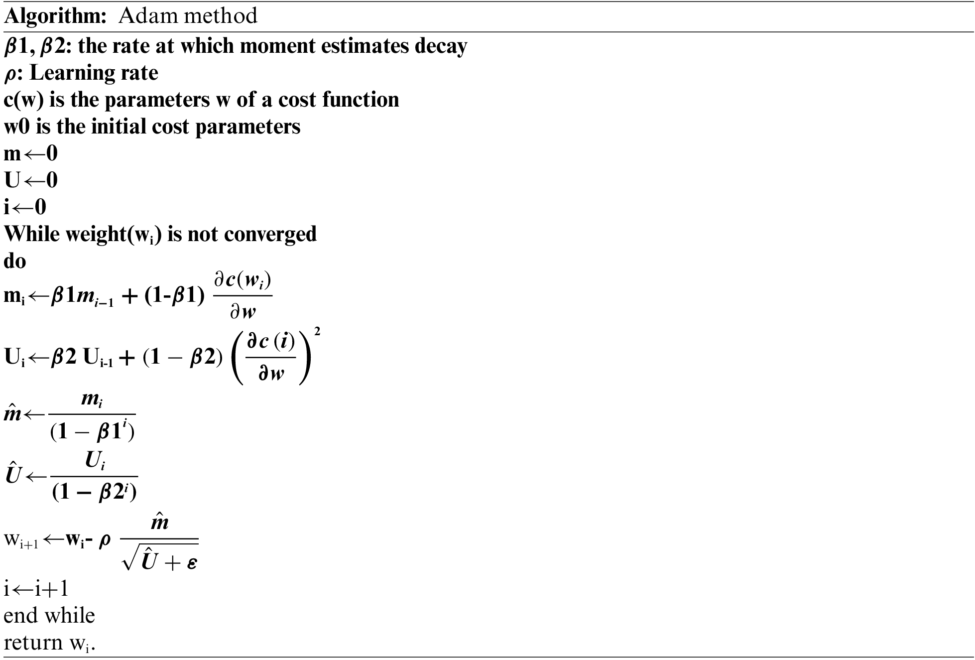
5.2 Weber Function on a Three-dimensional Surface, Only One Local Minimum
The two-variable function is used to in this section, so each approach impacts along parameters. The two-variable function utilized in this experiment (i.e., Weber function) is roughly defined as follows:
If
Fig. 1a, depicts the Weber function as a function of
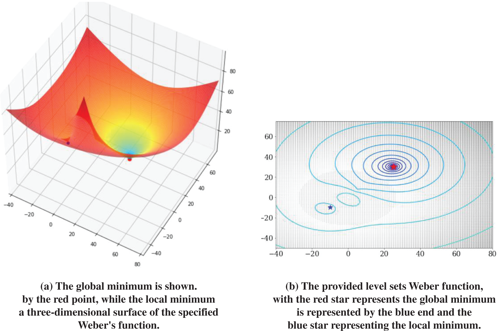
Figure 1:
Fig. 2, demonstrates how each method affects the parameters. We proposed a technique that avoided the local minimum to obtain the global minimum. In contrast, the Adam, Adagrad, and G.D. method moved the local minimum, which was close to the starting value, and were no longer reduced.
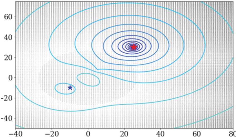
Figure 2: Visualization of each method’s changing parameters
5.3 Three Local Minimums on a Three-Dimensional Surface
The Tang–Styblinski Function performance of each technique was examined in this experimentation utilizing the Styblinski– Tang function as the cost function, with three the cost function is based on local minimums. The three local minima of the Styblinski–Tang function are specifically defined:
and it has a (−2.813,−2.813) global minimum. Fig. 3, follows the same pattern as the previous section.
Figure 3: Function of styblinski–tang
The initial parameter value is (7, 0), 1 × 10⁻² is the learning rate, and the learning has been done 301 times. Each strategy yielded a different modification in parameters as depicted in Fig. 4; Adagrad, GD, and Adam all headed towards to in this experiment. The local minimum is close to the original value, but, to achieve the global, our proposed technique avoided the local minimum.
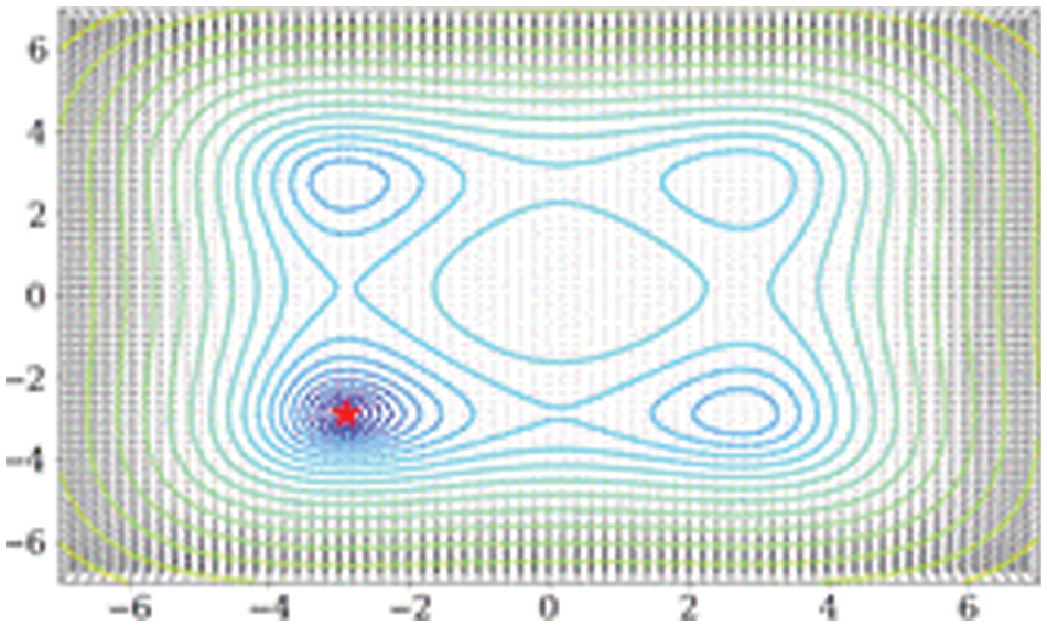
Figure 4: Visualization of each method’s parameters changing
5.4 MNIST with Convolution Neural Network (CNN)
The MNIST dataset is a 28 × 28 gray-scale picture with ten classes that are popular for machine learning; part of the MNIST data is shown in Fig. 5,
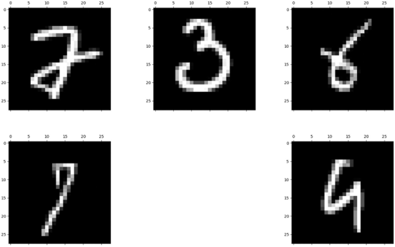
Figure 5: MNIST dataset examples
A basic structured CNN was utilized, with one hidden layer and two convolution layers to compare the performance of each approach. A 32 × 5 × 5 sized filter and a 64 × 32 × 5 × 5 sized filtering were used for the convolution; a 50% dropout was performed as well as the size of the batch was set to 64. The learning process was repeated 88300 times, with a learning rate of 0.0001. The experiment results are shown in Fig. 6.
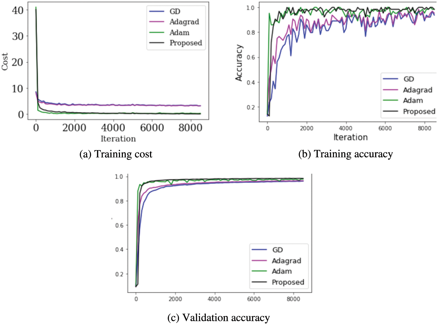
Figure 6: MNIST results using a CNN
Fig. 6a depicts the cost change as a function of learning using each approach, demonstrating that almost all strategies resulted in a cost reduction. Fig. 6b, shows the accuracy of the data gathered as the learning proceeds; in Fig. 6c, depicts the accuracy of validation as the learning progresses that uses the test data to see if it is over-fitting. Fig. 7, illustrates the accuracy after each iteration for comparison.
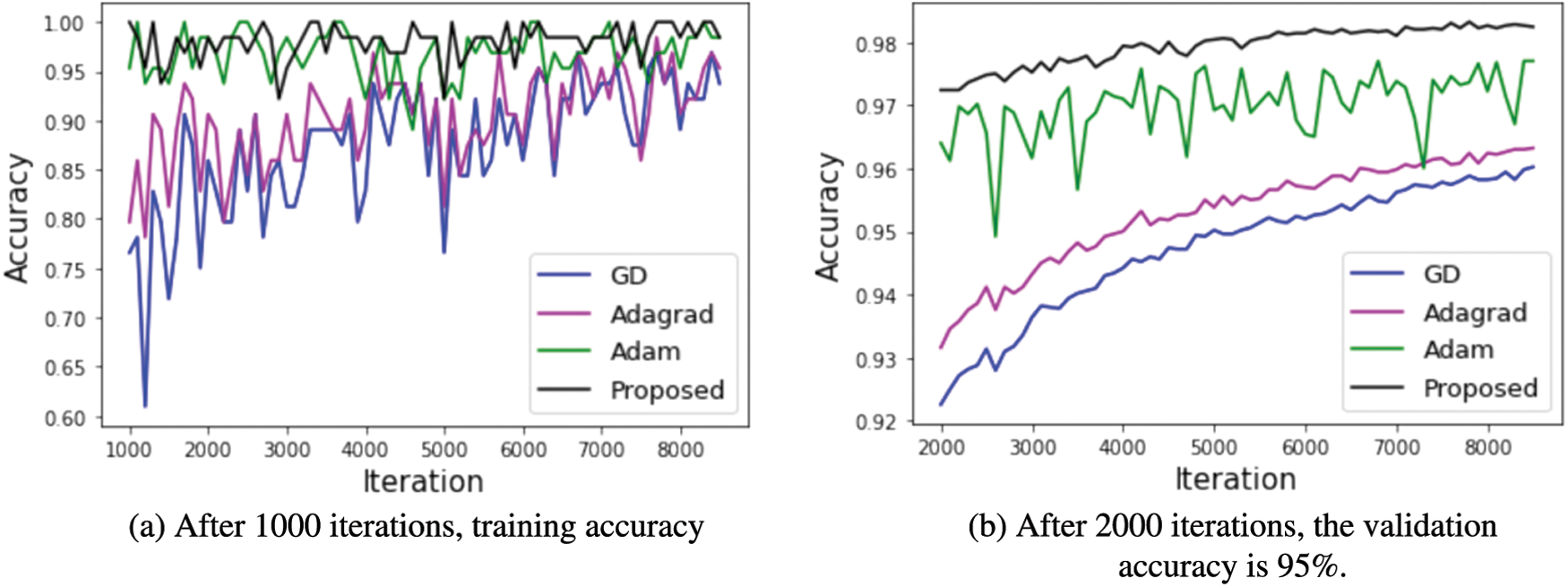
Figure 7: MNIST accuracy using convolution neural network
Fig. 7a depicts the training accuracy after 1000 iterations, whereas Fig. 7b shows the validation accuracy after 2000 iterations. All approaches have high training accuracy, but Adam and our proposed method had the highest validation accuracy.
CIFAR-10 dataset used to train in this section; we’ll use the RESNET model to examine more extensive tests of each method performance model. There were 60,000 images in the CIFAR-10 dataset. Color images from the CIFAR-10 collection were used, with ten different classes (trucks, airplanes, ships, vehicles, horses, frogs, dogs, deer, cats, and birds). The learning was done with the RESNET 44 model in 128 the batch size, 80,000 iterations, and 0.001 is a learning rate. The findings of each approach employed in this experiment are shown in Fig. 8.
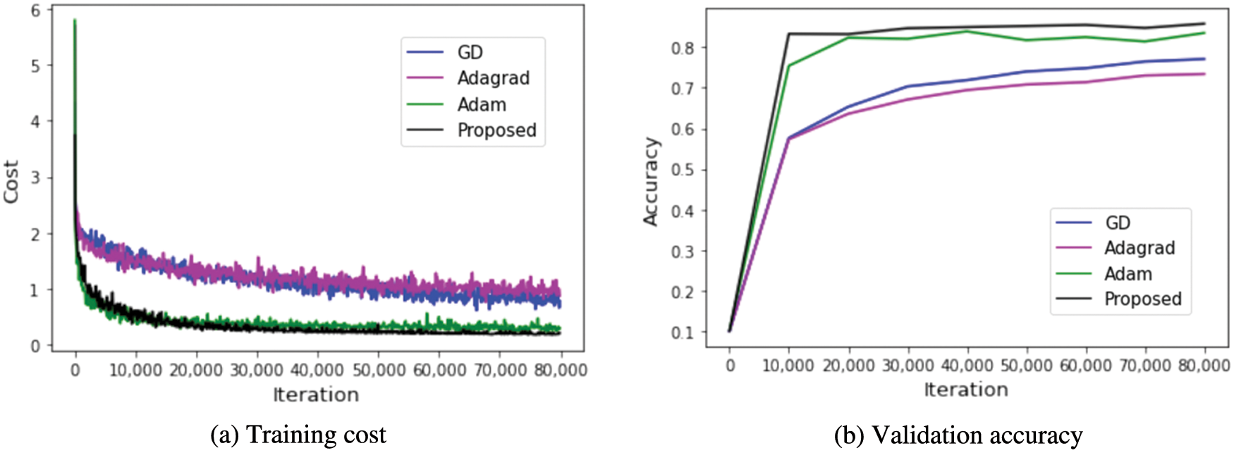
Figure 8: With a residual Network (RESNET), the results of the CIFAR-10 dataset
Fig. 8a depicts each method’s training cost, whereas Fig. 8b shows verification accuracy per 10,000 steps. Adam is the suggested technique with the minimum costs in Fig. 8a; our proposed method has little vibration. As a result, it appears to be a reliable learning strategy. Following the Adam method, the proposed method had the best performance in Fig. 8b.
6 Conclusions and Future Research Directions
We presented a deep learning method based on the current momentum approach that uses both of the first derivative and the same time of the cost function. In addition, our proposed strategy developed to learn in an optimal condition by modifying the learning rate technique that responds to cost function changes. The results of experimental shown this way of learning are Adam, GD, and momentum techniques used to validate our proposed strategy. According to studies, we confirmed pause learning in terms of successful learning because it leads to better learning accuracy than other techniques. The cost we define is zero if we use the global minimum of the cost function to converge to zero using our proposed method. It performs exceptionally well in terms of learning accuracy. Our approach provides several advantages because the learning rate is adaptive. Simply changing the formula may be used with existing learning methods. In the future, deep learning with a more profound arrangement will rate learning stop at a proper period in deep learning; stopping learning is a problem. On the other hand, it will be solved concurrently with practical learning.
Acknowledgement: Princess Nourah bint Abdulrahman University Researchers Supporting Project number (PNURSP2022R79), Princess Nourah bint Abdulrahman University, Riyadh, Saudi Arabia.
Funding Statement: This research is funded by Princess Nourah bint Abdulrahman University Researchers Supporting Project number (PNURSP2022R79), Princess Nourah bint Abdulrahman University, Riyadh, Saudi Arabia.
Conflicts of Interest: The authors declare that they have no conflicts of interest to report regarding the present study.
References
1. D. E. Rumelhart, G. E. Hinton and R. J. Williams, “Learning representations by back-propagating errors,” Nature, vol. 1986, no. 323, pp. 533–536, 1986. [Google Scholar]
2. A. K. Singha, A. Kumar and P. K. Kushwaha, “Cassification of brain tumors using deep encoder along with regression techniques,” EPH-International Journal of Science And Engineering, vol. 1, no. 1, pp. 444–449, 2018. [Google Scholar]
3. G. Hinton, L. Deng, D. Yu, G. E. Dahl, A. Mohamed et al., “Deep neural networks for acoustic modeling in speech recognition: The shared views of four research groups,” Signal Process. Mag, vol. 29, no. 6, pp. 82–97, 2012. [Google Scholar]
4. R. Pascanu and Y. Bengio, “Revisiting natural gradient for deep networks,” arXiv preprint arXiv, vol. 1301, pp. 3584, 2013. [Google Scholar]
5. A. K. Singha, N. Pathak, N. Sharma, A. Gandhar, S. Urooj et al., “An experimental approach to diagnose COVID-19 using optimized CNN,” Intelligent Automation and Soft Computing, vol. 34, no. 2, pp. 1066–1080, 2022. [Google Scholar]
6. G. E. Hinton, N. Srivastava, A. Krizhevs.y, I. Sutskever and R. R. Salakhutdinov, “Improving neural networks by preventing co-adaptation of feature detectors,” arXiv preprint arXiv, vol. 1207, pp. 580, 2012. [Google Scholar]
7. J. Sultana, Ak Singha, S. T. Siddiqui, G. Nagalaxmi, A. K. Sriram et al., “COVID-19 pandemic prediction and forecasting using machine learning classifiers,” Intelligent Automation and Soft Computing, vol. 32, no. 2, pp. 1007–1024, 2022. [Google Scholar]
8. C. T. Kelley, “Iterative methods for linear and nonlinear equations,” Frontiers in Applied Mathematics, vol. 34, pp. 1906–1994, 1995. [Google Scholar]
9. C. T. Kelley, “Iterative methods for optimization,” Frontiers in Applied Mathematics, vol. 23, pp. 161–177, 1999. [Google Scholar]
10. J. Duchi, E. Hazan and Y. Singer, “Adaptive sub gradient methods for online learning and stochastic optimization,” Journal of Machine Learning Research, vol. 12, pp. 2121–2159, 2011. [Google Scholar]
11. I. Sutskever, J. Martens, G. Dahl and G. E. Hinton, “On the importance of initialization and momentum in deep learning,” in Proc. of the 30th Int. Conf. on Machine Learning—ICML 2013, Atlanta, Georgia, USA, vol. 16–21, pp. 1139–1147, 2013. [Google Scholar]
12. M. D. Zeiler, “Adadelta: An adaptive learning rate method,” arXiv preprint arXiv, vol. 1212, pp. 5701, 2012. [Google Scholar]
13. D. P. Kingma and J. Ba, “ADAM: A method for stochastic optimization,” in Proc. of the 3rd Int. Conf. for Learning Representations—ICLR 2015, New York, USA, vol. 17–21, pp. 1213–1231, 2015. [Google Scholar]
14. S. J. Reddi, S. Kale and S. Kumar, “On the convergence of ADAM and beyond,” arXiv preprint arXiv, vol. 1904, pp. 9237, 2019. [Google Scholar]
15. L. Bottou, F. E. Curtis and J. Nocedal, “Optimization methods for large-scale machine learning,” Siam Review, vol. 60, no. 2, pp. 223–311, 2018. [Google Scholar]
16. Y. Nesterov, Introductory lectures on convex optimization: A basic course. Vol. 87. Berlin/Heidelberg, Germany: Springer, 2003. [Google Scholar]
17. S. Zubair and A. K. Singha, “Parameter optimization in convolutional neural networks using gradient descent,” Microservices in Big Data Analytics, vol. 2020, pp. 87–94, 2020. [Google Scholar]
18. R. Ge, S. M. Kakade, R. Kidambi and P. Netrapalli, “The step decay schedule: A near optimal, geometrically decaying learning rate procedure for least squares,” arXiv preprint arXiv, vol. 1904, pp. 12838, 2019. [Google Scholar]
19. S. Zubair and A. K. Singha, “Network in sequential form: Combine tree structure components into recurrent neural network,” IOP Conference Series: Materials Science and Engineering, vol. 1017, no. 1, pp. 12004, 2021. [Google Scholar]
20. Y. Yazan and M. F. Talu, “Comparison of the stochastic gradient descent based optimization techniques,” International Artificial Intelligence and Data Processing Symposium IEEE, vol. 16, pp. 1–5, 2017. [Google Scholar]
21. M. Chandra and M. Matthias, “Variants of RMSProp and adagrad with logarithmic regret bounds,” arXiv:1706.05507, 2017. [Google Scholar]
22. S. De, A. Mukherjee and E. Ullah, “Convergence guarantees for RMSProp and ADAM in nonconvex optimization and an empirical comparison to nesterov acceleration,” arXiv preprint arXiv, vol. 1807, pp. 6766, 2018. [Google Scholar]
23. E. M. Dogo, O. J. Afolabi, N. I. Nwulu, B. Twala and C. O. Aigbavboa, “A comparative analysis of gradient descent-based optimization algorithms on convolutional neural networks,” in Int. Conf. on Computational Techniques, Electronics and Mechanical Systems, Udyambag, India, vol. 2018, pp. 92–99, 2018. [Google Scholar]
24. S. Voronov, I. Voronov and R. Kovalenko, “Comparative analysis of stochastic optimization algorithms for image registration,” in IV Int. Conf. on Information Technology and Nanotechnology, Molodogvardeyskaya St, Russia, vol. 12, pp. 21–23, 2018. [Google Scholar]
25. J. Duchi, E. Hazan and Y. Singer, “Adaptive subgradient methods for online learning and stochastic optimization,” Journal of Machine Learning Research, vol. 12, no. 7,pp, pp. 257–269, 2011. [Google Scholar]
26. Z. Hui, C. Zaiyi, Q. Chuan, H. Zai, W. Z. Vincent et al., “Adam revisited: A weighted past gradients perspective Front,” Frontiers of Computer Science, vol. 14, no. 5, pp. 1–16, 2020. [Google Scholar]
27. S. Yousefi, E. Yousefi, H. Takahashi, T. Hayashi, H. Tampo et al., “Keratoconus severity identification using unsupervised machine learning,” PLOS ONE, vol. 13, no. 11, pp. e0205998, 2018. [Google Scholar]
28. A. K. Singha, A. Kumar and P. K. Kushwaha, “Speed predication of wind using Artificial neural network,” EPH-International Journal of Science And Engineering, vol. 1, no. 1, pp. 463–469, 2018. [Google Scholar]
29. T. Tieleman and G. E. Hinton, Lecture 6.5—RMSProp,coursera: Neural networks for machine learning. Toronto: University of Toronto, 2012. [Google Scholar]
30. A. K. Singha, Anil Kumar, and P. K. Kushwaha, “Recognition of human layered structure using gradient decent model,” EPH International Journal of Science and Engineering, vol. 1, no. 1, pp. 450–456, 2018. https://.doi.org/10.53555/ephse.v1i1.1295. [Google Scholar]
31. A. K. Singha, A. Kumar and P. K. Kushwaha, “Recognition of human layered structure using gradient decent model,” EPH-International Journal of Science And Engineering, vol. 1, no. 1, pp. 450–456, 2018. [Google Scholar]
32. Y. LeCum, Y. Bengio and G. Hinton, “Deep learning,” Nature, vol. 521, no. 7553, pp. 436–444, 2015. [Google Scholar]
33. D. Yi, J. Ahn and S. Ji, “An effective optimization method for machine learning based on ADAM,” Applied Sciences, vol. 10, no. 3, pp. 1073–1092, 2020. [Google Scholar]
34. A. Krizhevsky, I. Sutskever and G. E. Hinton, “Imagenet classification with deep convolutional neural networks,” in Proc. of the Neural Information Processing Systems, CA, USA, vol. 3–6, pp. 1097–1105, 2017. [Google Scholar]
Cite This Article
 Copyright © 2023 The Author(s). Published by Tech Science Press.
This work is licensed under a Creative Commons Attribution 4.0 International License , which permits unrestricted use, distribution, and reproduction in any medium, provided the original work is properly cited.
 Downloads
 Citation Tools